Permanent address.]

Spin swap gate in the presence of qubit inhomogeneity in a double quantum dot

Abstract

We study theoretically the effects of qubit inhomogeneity on the quantum logic gate of qubit swap, which is an integral part of the operations of a quantum computer. Our focus here is to construct a robust pulse sequence for swap operation in the simultaneous presence of Zeeman inhomogeneity for quantum dot trapped electron spins and the finite-time ramp-up of exchange coupling in a double dot. We first present a geometric explanation of spin swap operation, mapping the two-qubit operation onto a single-qubit rotation. We then show that in this geometric picture a square-pulse-sequence can be easily designed to perform swap in the presence of Zeeman inhomogeneity. Finally, we investigate how finite ramp-up times for the exchange coupling $J$ negatively affect the performance of the swap gate sequence, and show how to correct the problems numerically.

The study of quantum information processing has attracted a great deal of attention in recent years because of the potential advantages provided by quantum mechanical principles such as superposition and entanglement Reviews . Among the many proposed quantum computer (QC) architectures, solid-state schemes such as those based on electron LD ; Vrijen and nuclear spins Kane and those based on superconducting circuits Schon are widely regarded as the best candidates in providing scalable systems. However, solid-state architectures also have their own shortcomings. For example, in supeconducting-circuit-based QC schemes, offset charge noise due to jumps of trapped charges has been an important limiting factor Nakamura ; charge_echo ; Saclay ; In semiconductors such as silicon, complexities in their band structures can potentially lead to significant difficulties in qubit manipulations BHD . The often small energy scales in solids lead to slower coherent operations and harder initializations. Furthermore, in many solid-state QC schemes it is almost impossible to have completely identical qubits. As potential and problems coexist in proposed solid-state QC architectures, theoretical explorations are sorely needed to provide effective forewarnings and guidelines. In particular, it is important to analyze theoretically various possible sources of errors (arising, for example, from imperfection, inhomogeneity, decoherence, nonadiabaticity, and in general from deviations from ideal architectures assumed in the QC proposals which must invariably be present in real solid-state systems) in these solid-state QC schemes. For example, In the spin-based quantum dot quantum computer (QDQC) architecture LD ; BLD ; HD ; Revs , where trapped electron spins are the quantum bits (qubits), quantum dots provide the tags and the environment for the individual qubits. Each quantum dot is generally slightly different in size, geometry, confinement potential depth, g factors, etc. Some of these differences can be accounted for straightforwardly by system calibration, while others, such as inhomogeneity in the electron spin Zeeman splitting, have to be treated more carefully.

In this paper we study how to overcome the problems arising from qubit inhomogeneity and gate imperfections in the spin-based QDQC, particularly focusing on the swap operation. It is important to emphasize here that in realistic QC architectures, two-qubit operations include not only the entangling operations such as controlled-NOT, but also auxilliary operations such as swap, which are crucial components for the effective manipulation of a QC (the function of swap in QDQC is to move non-neighboring qubits together and apart through a quantum dot array during entangling operations). Furthermore, controlled-NOT operation in QDQC is built upon the square-root-of-swap operations. Therefore, imperfections that affect swap will also affect controlled-NOT in general. For instance, previously we have shown that swap operation LD cannot be done precisely in one step if there is inhomogeneity in the electron Zeeman splitting HSD , because the inhomogeneity breaks the symmetry of the two-spin system. Here we first present a geometric interpretation of two-spin swap operation in terms of single spin rotation, and design a square pulse sequence to perform swap in the presence of Zeeman inhomogeneity. We then discuss the effects of qubit inhomogeneity and imperfect control of the exchange coupling on the swap gate sequence, and present its numerically corrected version.

Under the condition that the double quantum dot low-energy dynamics can be described by Heisenberg exchange Hamiltonian HD ; Gate , the two-electron spin Hamiltonian can be written as a sum of the exchange term and the Zeeman splittings:

$$H=J{\bf S}_{1}\cdot{\bf S}_{2}+\gamma_{1}S_{1z}+\gamma_{2}S_{2z}\,,$$ (1)

where $J$ gives the strength of exchange coupling and is a function of quantum dot size, geometry, and confinement. $\gamma_{1}$ and $\gamma_{2}$ are the Zeeman splittings of the two spins and are functions of local g factors and magnetic fields. If we express this Hamiltonian on the two-spin basis $|\uparrow\uparrow\rangle$, $|\uparrow\downarrow\rangle$, $|\downarrow\uparrow\rangle$, and $|\downarrow\downarrow\rangle$, and let $\delta=\gamma_{1}-\gamma_{2}$ be the Zeeman inhomogeneity and $\gamma=(\gamma_{1}+\gamma_{2})/2$ the average Zeeman coupling, we obtain

$$H=\left(\begin{array}[]{cccc}2\gamma&0&0&0\\ 0&\delta&J&0\\ 0&J&-\delta&0\\ 0&0&0&-2\gamma\end{array}\right)\,,$$ (2)

Notice that within this Hamiltonian the two unpolarized states $|\uparrow\downarrow\rangle$ and $|\downarrow\uparrow\rangle$ are decoupled from the two polarized states $|\uparrow\uparrow\rangle$ and $|\downarrow\downarrow\rangle$, thus their dynamics can be described separately.

To understand how swap works, we first write down the spin states before and after a swap:

$$\left(\begin{array}[]{c}\alpha_{1}\\ \alpha_{2}\end{array}\right)\otimes\left(\begin{array}[]{c}\beta_{1}\\ \beta_{2}\end{array}\right) = \alpha_{1}\beta_{1}|\uparrow\uparrow\rangle+\alpha_{2}\beta_{2}|\downarrow\downarrow\rangle+\alpha_{1}\beta_{2}|\uparrow\downarrow\rangle+\alpha_{2}\beta_{1}|\downarrow\uparrow\rangle$$

$$= \alpha_{1}\beta_{1}T_{\uparrow}+\alpha_{2}\beta_{2}T_{\downarrow}+\frac{\alpha_{1}\beta_{2}+\alpha_{2}\beta_{1}}{\sqrt{2}}T_{0}+\frac{\alpha_{1}\beta_{2}-\alpha_{2}\beta_{1}}{\sqrt{2}}S\,.$$

$$\left(\begin{array}[]{c}\beta_{1}\\ \beta_{2}\end{array}\right)\otimes\left(\begin{array}[]{c}\alpha_{1}\\ \alpha_{2}\end{array}\right) = \alpha_{1}\beta_{1}|\uparrow\uparrow\rangle+\alpha_{2}\beta_{2}|\downarrow\downarrow\rangle+\alpha_{2}\beta_{1}|\uparrow\downarrow\rangle+\alpha_{1}\beta_{2}|\downarrow\uparrow\rangle$$

$$= \alpha_{1}\beta_{1}T_{\uparrow}+\alpha_{2}\beta_{2}T_{\downarrow}+\frac{\alpha_{1}\beta_{2}+\alpha_{2}\beta_{1}}{\sqrt{2}}T_{0}-\frac{\alpha_{1}\beta_{2}-\alpha_{2}\beta_{1}}{\sqrt{2}}S\,,$$

where $T_{\uparrow}=|\uparrow\uparrow\rangle$, $T_{\downarrow}=|\downarrow\downarrow\rangle$, and $T_{0}=(|\uparrow\downarrow\rangle+|\downarrow\uparrow\rangle)/\sqrt{2}$ are the triplet states, while $S=(|\uparrow\downarrow\rangle-|\downarrow\uparrow\rangle)/\sqrt{2}$ is the two-spin singlet state. From the above expressions, swap is achieved by switching the coefficients of the unpolarized $|\uparrow\downarrow\rangle$ and $|\downarrow\uparrow\rangle$ states, or equivalently, changing the coefficient of the singlet component by a $\pi$ phase shift relative to the triplet states. The phase shift can be easily obtained by a Heisenberg exchange Hamiltonian $H=J{\bf S}_{1}\cdot{\bf S}_{2}$, since singlet and triplet states are the eigenstates of the exchange Hamiltonian (split by $4J$) so that its only effect is to introduce dynamical phases to each basis state.

If a uniform magnetic field is present ($\gamma_{1}=\gamma_{2}=\gamma$), the triplet states are split by the Zeeman coupling $\gamma$. When the exchange Hamiltonian is applied to the two-spin system together with the uniform magnetic field, swap can still be performed, with an additional phase: instead of an exact swap, now the final states take on the form

$$\left(\begin{array}[]{c}\alpha_{1}\\ \alpha_{2}\end{array}\right)\otimes\left(\begin{array}[]{c}\beta_{1}\\ \beta_{2}\end{array}\right)\rightarrow\left(\begin{array}[]{c}\beta_{1}e^{i\gamma t/\hbar}\\ \beta_{2}e^{-i\gamma t/\hbar}\end{array}\right)\otimes\left(\begin{array}[]{c}\alpha_{1}e^{i\gamma t/\hbar}\\ \alpha_{2}e^{-i\gamma t/\hbar}\end{array}\right)\,.$$ (13)

In other words, different spin states acquire different phases depending on their Zeeman energies HSD . Thus the additional phases here come only from the polarized states.

When there is Zeeman inhomogeneity between the two quantum dots, the spin dynamics is more complicated since the singlet and unpolarized triplet states are coupled by the inhomogeneous Zeeman splitting. However, as we mentioned before, within Hamiltonian (1) the dynamics of the polarized and unpolarized two-spin states are separated. With the polarized states still eigenstates of Hamiltonian (1), we need to focus on only the unpolarized states $|\uparrow\downarrow\rangle$ and $|\downarrow\uparrow\rangle$. Since these states are not coupled to the polarized states, the two-state subspace they span can be treated as an effective spin-$1/2$ system with an effective Hamiltonian note

$$H_{e}=\left(\begin{array}[]{cc}\delta&J\\ J&-\delta\end{array}\right)=J\sigma_{x}+\delta\sigma_{z}=J_{n}\hat{n}\cdot\mbox{\boldmath$\sigma$}\,,$$ (14)

where $J_{n}=\sqrt{J^{2}+\delta^{2}}$ and $\hat{n}=(J,0,\delta)/J_{n}$. Within the picture of this effective spin-$1/2$ system, there is a simple geometric explanation to the two-spin swap operation. Hamiltonian (14) is a rotation on the Bloch sphere of the effective spin-$1/2$ system around the axis given by $\hat{n}$, with the rotation angle being determined by the duration and strength of this Hamiltonian. In the absence of inhomogeneity ($\delta=0$), the rotation is around the $x$ axis. Thus a $\pi$ rotation for this effective spin-$1/2$ system would correspond preceisely to a “swap” in the original two-qubit system: $|\uparrow\downarrow\rangle\rightarrow|\downarrow\uparrow\rangle$ and $|\downarrow\uparrow\rangle\rightarrow|\uparrow\downarrow\rangle$.

In the presence of Zeeman inhomogeneity, the rotational axis $\hat{n}$ deviates away from the $x$ axis. Now starting from the north pole of the Bloch sphere, the state will not be able to reach the south pole by one rotation around a fixed axis (corresponding to a square pulse of exchange coupling in the presence of inhomogeneity). Thus, Zeeman inhomogeneity makes the exact swap impossible by a single pulse of $J$ (with a fixed sign) HSD . However, swap can still be performed if the Zeeman inhomogeneity is known (for example, if it is due to engineered g-factor). Essentially, we can adjust the rotational axis by changing the magnitude of the exchange coupling $J$. For example, we can switch on a square pulse of exchange with magnitude $J$ for a $\pi$ rotation, then turn off the exchange and let the system undergo a $\pi$ rotation around the $z$ axis (driven by the inhomogeneous Zeeman splitting), then switch on a second square pulse of exchange with magnitude $J^{\prime}=\delta^{2}/J$ for a $\pi$ rotation. If we define $R(\hat{n},\theta)$ to be a $\theta$-rotation around the $\hat{n}$ direction, the pulse sequence for swap would be:

$$U_{\rm swap}=R(\hat{n},\pi)\,R(\hat{z},\pi)\,R(\hat{n}^{\prime},\pi)\,,$$ (15)

where the rotational axis are $\hat{n}=(J,0,\delta)/\sqrt{J^{2}+\delta^{2}}$, $\hat{z}=(0,0,1)$, and $\hat{n}^{\prime}=(J^{\prime},0,\delta)/\sqrt{J^{\prime\,2}+\delta^{2}}$. The end result of this pulse sequence would be a swap for the two spins: $|\uparrow\downarrow\rangle\leftrightarrow|\downarrow\uparrow\rangle$. Figure 1 shows a schematic comparison of the square pulse sequence in the absence and presence of Zeeman inhomogeneity. If in the above pulse sequence the exchange couplings $J$ or $J^{\prime}$ is unphysically large, we can always use smaller exchange couplings instead, but with a longer pulse sequence. For example, if $J$ is the maximal exchange while $J^{\prime}$ is even bigger (which implies a large Zeeman inhomogeneity $\delta$), we can keep performing $R(\hat{n},\pi)\,R(\hat{z},\pi)$ until at last a $R(\hat{n}^{\prime},\pi)$ with $J^{\prime}<J$ can be used to complete the sequence ($J^{\prime}$ is determined uniquely by $J$ and $\delta$):

$$U_{\rm swap}=R(\hat{n},\pi)\,R(\hat{z},\pi)\,R(\hat{n},\pi)\,R(\hat{z},\pi)\cdots\,R(\hat{n}^{\prime},\pi)\,.$$ (16)

Take a simple example of $J/\delta=\tan(\pi/8)=\sqrt{2}-1$ with $J$ being the largest possible physical value, the pulse sequence for swap is

$$U_{\rm swap}=R(\hat{n},\pi)\,R(\hat{z},\pi)\,R(\hat{n},\pi)\,R(\hat{z},\pi)\,R(\hat{n},\pi)\,R(\hat{z},\pi)\,R(\hat{n},\pi)\,,$$ (17)

which invokes the exchange coupling $4$ times. This simply shows that exchange becomes less efficient in performing swap operation if Zeeman inhomogeneity is large. An alternative interaction might have to be used instead (such as optically assisted spin flip).

Using the geometric picture for swap, it is apparent that the presence of inhomogeneous Zeeman splitting introduces additional complexities to swap operation. For instance, in the absence of Zeeman inhomogeneity, it does not matter whether the exchange coupling $J$ is switched on suddenly or gradually as the rotational axis is always fixed along $x$; while in the presence of Zeeman inhomogeneity, swap operation cannot be done for two spins (or, flip cannot be achieved for the effective spin-1/2) in one shot. The introduction of a finite pulse rise/fall time aggravates this problem as the orientation of the rotational axis of the effective spin-1/2 system becomes time-dependent (a gradually switched-on exchange coupling means that the rotational axis is time-dependent for the switch-on period, which immediately leads to incomplete and/or imprecise rotations). To quantify this difference we perform a numerical calculation and show that the shift in rotational axis reduces the efficiency of exchange coupling in performing swap operations. We then numerically search for the appropriate exchange coupling to perform swap operation under these non-ideal conditions.

In the following we use the square pulse case (sharp rise and fall of the exchange coupling) as a benchmark to measure the degradation of the rotation by the exchange pulses with finite rise/fall times and introduce an effective infidelity $\Delta\sigma_{z}=\left.\sigma_{z}\right|_{\rm opt}-\sigma_{0}$, where $\sigma_{0}$ is the smallest $\sigma_{z}$ reached by a square exchange pulse after a $\pi$ rotation starting from the north pole of the Bloch sphere, while $\left.\sigma_{z}\right|_{\rm opt}$ is the smallest $\sigma_{z}$ reached by an exchange pulse with finite $\tau_{r}$ and optimized pulse duration (not necessarily a $\pi$ pulse, which is ill-defined for a time-dependent axis anyway). Fig. 2 gives several trajectories for optimized rotation on the Bloch sphere projected onto the $xy$ plane. Each trajectory represents a case with a chosen pulse rise/fall time and an optimized pulse duration so that the final destination point has the smallest $\langle\sigma_{z}\rangle$ component (closest to the $\langle\sigma_{z}\rangle=-1$ south pole point. Recall that a rotation from the north pole to the south pole and vice versa corresponds to an exact swap: $|\uparrow\downarrow\rangle\leftrightarrow|\downarrow\uparrow\rangle$). All the curves share a common exchange coupling $J=0.2$meV and an inhomogeneity of $\delta=0.1$meV. One interesting feature here is that when the pulse rise/fall time is sufficiently long (5ps in this case), the system has to undergo approximately one and a half full rotation (instead of one half full rotation, or the $\pi$-pulse) in order to reach the smallest $\langle\sigma_{z}\rangle$. In addition, notice that these optimal rotations are generally not $\pi$-rotations anymore.

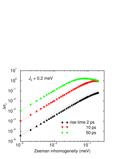
Figure 4: Single pulse swap infidelity $\Delta\sigma_{z}$ as a function of Zeeman inhomogeneity at a fixed exchange coupling $J$ and three different pulse rise times.

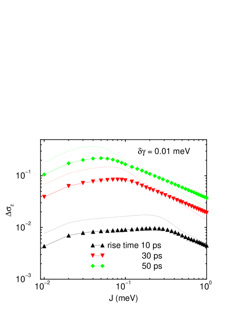
Figure 5: Single pulse swap infidelity $\Delta\sigma_{z}$ as a function of the exchange coupling $J$ at a fixed Zeeman inhomogeneity and three different pulse rise times.

In Figures 3, 4, and 5, we show how the efficiency of an exchange pulse in performing rotations varies with the exchange coupling $J$, Zeeman inhomogeneity $\delta$, and the pulse rise/fall time $\tau_{r}$. In these figures, the filled and unfilled symbols correspond to two different pulse shapes: sinusoidal and linear rise/fall, respectively. For the sinusoidal rise, $J=J_{M}sin^{2}(\pi t/2\tau_{r})$, while for the linear rise, $J=J_{M}t/\tau_{r}$, where $J_{M}$ is the maximal exchange couping during the pulse.

In Fig. 3 we plot the effective infidelity $\Delta\sigma_{z}$ as a function of the pulse rise/fall time when the maximum exchange is set at $0.2$meV. There are four sets (each with two pulse shapes) of data shown in the figure corresponding to four different values of Zeeman inhomogeneity, as indicated in the legend. At small pulse rise/fall time $\tau$, the infidelity $\Delta\sigma_{z}$ grows approximately as a quadratic function of $\tau$ (below $\sim 10$ps) for both pulse shape. At longer $\tau$ the growth saturates since the maximum value of $\Delta\sigma_{z}$ is 2. In Fig. 4 we plot the effective infidelity $\Delta\sigma_{z}$ as a function of the Zeeman inhomogeneity at a fixed exchange coupling $J=0.2$meV and three different pulse rise times. Similar to Fig. 3, the infidelity grows quadratically (for both pulse shapes) with inhomogeneity, then saturates when the inhomogeneity is in the same order of magnitude as the exchange coupling. The quadratic behavior in both Fig. 3 and Fig. 4 might be understood as the result of small parameter Taylor expansions. In Fig. 5, the infidelity $\Delta\sigma_{z}$ is plotted as a function of the maximum exchange coupling $J$ at a fixed inhomogeneity $\delta\gamma=0.01$meV and three different pulse rise times. Here for the two different pulse shapes the infidelity decreases with different power law as the exchange coupling $J$ increases, essentially because the larger exchange coupling leads to an enhanced role played by the time-dependent function of the pulse shape.

It is clear from Figs. 3 to 5 that imperfect exchange pulses (or non-square pulses) in the presence of Zeeman inhomogeneity reduce the effectiveness of the exchange interaction in performing swap operation. The key question now is whether one can still perform swap operations when square pulses are not available. The answer is affirmative. In analogy to the square pulse case shown in Fig. 1, one can turn on the most efficient exchange pulse as shown above, then let the system freely evolve (in the presence of Zeeman inhomogeneity) an optimal period of time, then turn on an exchange pulse again. Now each of the pulses is generally not an exact $\pi$ pulse, but have to be calculated numerically to last for the most efficient duration. Similar to the square pulse case, such pulse sequence might have to be used more than once if the Zeeman inhomogeneity is too large while the exchange coupling strength is weak. However, in many realistic situations, some numerical corrections to the pulse sequence shown in Fig. 1 should be sufficient to produce a precise swap operation. In Table 1 we summarize three different situations.

Pulse sequence	1	2	3
Zeeman inhomogeneity (meV)	0.1	0.1	0.01
pulse rise time (ps)	5	10	5
1st exchange coupling (meV)	0.2	0.2	0.2
2nd exchange coupling (meV)	0.0965	0.677	0.000605
corrections to the 2nd pulse (meV)	+0.0465	+0.672	+0.000105
fidelity	0.999998	0.999994	0.9999999

Table 1: Numerically obtained pulse sequences for various exchange pulses to achieve a complete swap. Notice that in each of the cases the strength of the second exchange pulse increases, by 93%, 12.5 times, and 20%, respectively.

Here we can see that longer pulse rise time leads to significantly higher requirement for large exchange interaction. In the case of the first and second pulse sequences, if the pulses are square, the magnitude of the second exchange pulse needs to be $\delta^{2}/J=0.05$ meV. When the pulse rise time is 5 ps, this magnitude nearly doubles; while a 10 ps rise time leads to a large exchange coupling of 0.677 meV, more than ten times bigger than the square pulse case. If the maximum exchange is below 0.5 meV, a swap would require several pulses to perform (as in Eq. (16)), so that the operation becomes less efficient. To further illustrate this point, we plot the strength of the second exchange pulse $J^{\prime}$ in the 3-pulse swap sequence of Eq. (15) as a function of the pulse rise time in Fig. 6. The unit for $J^{\prime}$ is its value in the square pulse case: $\delta^{2}/J_{0}$ where $\delta$ is the Zeeman inhomogeneity and $J_{0}$ is the strength of the first exchange pulse (with the same pulse rise time for simplicity). It is quite clear from Fig. 6 that the required strength for the second exchange pulse increases exponentially with the pulse rise time. For example, at 15 ps pulse rise time, the required $J^{\prime}$ is above 2.8 meV (as compared to 0.05 meV in the square pulse case), beyond the range available in the current state-of-the-art double dots. Multi-pulse sequences as in Eq. (16) would have to be invoked in such scenarios.

In summary, we have assessed the effects of qubit inhomogeneity on the swap operations in a quantum dot quantum computer. We have shown that the exchange Hamiltonian becomes less efficient in performing swap when qubit inhomogeneity is present and the exchange is not turned on and off in the ideal square pulse shape. We have demonstrated ways to perform complete swap, at the expense of longer pulse sequences and numerically-searched pulse parameters zerofield . In exchange-based quantum computing schemes, entangling operations such as controlled-NOT are constructed from the square root of swap operation. With the extra complexity in the swap operation in the currently studied situation, it is quite natural to expect more complexity in controlled-NOT operations as well. Furthermore, since our calculation is performed in an effective two-level system, our results are applicable to single qubit operations, too. In essence, if $|0\rangle$ and $|1\rangle$ states are split energetically, attempts to perform direct rotations around axes other than $z$ will be hindered if that interaction is turned on and off gradually instead of in a square pulse profile. Indeed, the effects of such non-ideal pulses have been explored in solid-state systems like Cooper pair boxes Choi ; Oh ; Gate and charge oscillations in double quantum dots Fuji1 ; Fuji2 ; Fuji3 , and will surely be encountered even more in the future experimental studies of various solid-state quantum computing architectures.

This work is supported by ARDA and LPS.

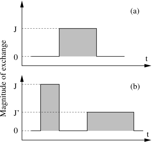
Figure 1: Square pulse sequences for a swap operation. (a) In the absence of Zeeman inhomogeneity, swap can be achieved by a $\pi$ pulse of the exchange interaction; (b) In the presence of Zeeman inhomogeneity $\delta$, swap can be achieved by two $\pi$ pulses of the exchange interaction with magnitudes $J$ and $J^{\prime}=\delta^{2}/J$, and a $\pi$ pulse for free evolution with $\delta$ in between.

Figure 2: Sample trajectories of rotations on the Bloch sphere of the effective spin-$1/2$ system performed by single exchange pulses and projected onto the $xy$ plane.

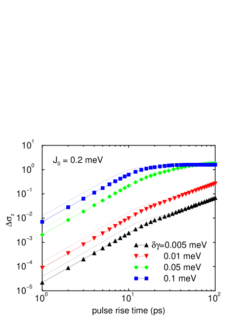
Figure 3: Single pulse swap infidelity $\Delta\sigma_{z}$ as a function of pulse rise time at a fixed exchange coupling $J$ and four different Zeeman inhomogeneities. In this figure and the two following ones, the dashed lines without symbols represent data for trapezoidal pulse shape (linear rise/fall), while the solid lines with symbols are for a sinusoidal pulse rise/fall.

Figure 6: Strength of the second exchange pulse in a complete swap pulse sequence as a function of the pulse rise time. The first exchange pulse strength is set at 0.2 meV while Zeeman inhomogeneity is 0.1 meV.

References

- (1) C.H. Bennett and D.P. DiVincenzo, Nature (London) 404, 247 (2000).
- (2) D. Loss and D.P. DiVincenzo, Phys. Rev. A 57, 120 (1998).
- (3) R. Vrijen, E. Yablonovitch, K. Wang, H.W. Jiang, A. Balandin, V. Roychowdhury, T. Mor, and D.P. DiVincenzo, Phys. Rev. A 62, 012306 (2000).
- (4) B.E. Kane, Nature (London) 393, 133 (1998); V. Privman, I.D. Vagner, and G. Kventsel, Phys. Lett. A 239, 141 (1998).
- (5) A. Shnirman, G. Schön, and Z. Hermon, Phys. Rev. Lett. 79, 2371 (1997); D.V. Averin, Solid State Commun. 105, 659 (1998).
- (6) Y. Nakamura, Y.A. Pashkin, and J.S. Tsai, Nature (London) 398, 786 (1999).
- (7) Y. Nakamura, Y.A. Pashkin, T. Yamamoto, and J.S. Tsai, Phys. Rev. Lett. 88, 047901 (2002).
- (8) D. Vion, A. Aassime, A. Cottet, P. Joyez, H. Pothier, C. Urbina, D. Esteve, and M.H. Devoret, Science 296, 886 (2002).
- (9) B. Koiller, X. Hu, and S. Das Sarma, Phys. Rev. Lett. 88, 027903 (2002).
- (10) G. Burkard, D. Loss, and D.P. DiVincenzo, Phys. Rev. B 59, 2070 (1999).
- (11) X. Hu and S. Das Sarma, Phys. Rev. A 61, 062301 (2000).
- (12) X. Hu and S. Das Sarma, in Experimental Implementation of Quantum Computation (IQC’01), ed. by R.G. Clark (Rinton, Princeton, 2001), cond-mat/0102019; cond-mat/0207457, to appear in the Proceedings of MQC2; Phys. Stat. Sol. (b) 238, 260 (2003) and cond-mat/0211358.
- (13) X. Hu, R. de Sousa, and S. Das Sarma, Phys. Rev. Lett. 86, 918 (2001).
- (14) X. Hu and S. Das Sarma, Phys. Rev. A 66, 012312 (2002).
- (15) The study of this effective spin- system has been done in the context of Ref. Levy in terms of square pulses Geometric , while we in this paper focus on the geometric explanation of swap and the effects of the nonsquare pulses.
- (16) J. Levy, Phys. Rev. Lett. 89, 147902 (2002).
- (17) S.C. Benjamin, Phys. Rev. A 64, 054303 (2001).
- (18) Alternative approaches (such as turning off the applied magnetic field), which go beyond the scope of the current study, can be designed to overcome the problem caused by inhomogeneous Zeeman splittings.
- (19) M.-S. Choi, R. Fazio, J. Siewert, and C. Bruder, Europhys. Lett. 53, 251 (2001).
- (20) S. Oh, Phys. Rev. B 65, 144526 (2002).
- (21) T. Fujisawa, Y. Tokura, and Y. Hirayama, Phys. Rev. B 63, 081304 (2001).
- (22) T. Fujisawa, D.G. Austing, Y. Tokura, Y. Hirayama, and S. Tarucha, Nature (London) 419, 278 (2002).
- (23) T. Hayashi, T. Fujisawa, H.D. Cheong, Y.H. Jeong, and Y. Hirayama, cond-mat/0308362.