Formulae for zero-temperature conductance through a region with interaction

Abstract

The zero-temperature linear response conductance through an interacting mesoscopic region attached to noninteracting leads is investigated. We present a set of formulae expressing the conductance in terms of the ground-state energy or persistent currents in an auxiliary system, namely a ring threaded by a magnetic flux and containing the correlated electron region. We first derive the conductance formulae for the noninteracting case and then give arguments why the formalism is also correct in the interacting case if the ground state of a system exhibits Fermi liquid properties. We prove that in such systems, the ground-state energy is a universal function of the magnetic flux, where the conductance is the only parameter. The method is tested by comparing its predictions with exact results and results of other methods for problems such as the transport through single and double quantum dots containing interacting electrons. The comparisons show an excellent quantitative agreement.

I introduction

The measurements of the conductivity and the electron transport in general are one of the most direct and sensitive probes in solid state physics. In such measurements many interesting new phenomena were signaled, in particular superconductivity, transport in metals with embedded magnetic impurities and the related Kondo physics, heavy fermion phenomena and the physics of the Mott-Hubbard transition regime. In the last decade technological advances enabled controlled fabrication of small regions connected to leads and the conductance, relating the current through such a region to the voltage applied between the leads, also proved to be a relevant property of such systems. There is a number of such examples, e.g. metallic islands prepared by e-beam lithography or small metallic grains Delft01 , semiconductor quantum dots Kouwenhoven97 , or a single large molecule such as a carbon nanotube or DNA. It is possible to break a metallic contact and measure the transport properties of an atomic-size bridge that forms in the breakAgrait02 , or even measure the conductance of a single hydrogen molecule, as reported recently in Ref. Smit02 . In all such systems, strong electron correlations are expected to play an important role.

The transport in noninteracting mesoscopic systems is theoretically well described in the framework of the Landauer-Büttiker formalism. The conductance is determined with the Landauer-Büttiker formula Landauer57 ; Landauer70 ; Buttiker86 , where the key quantity is the single particle transmission amplitude $t(\varepsilon)$ for electrons in the vicinity of the Fermi energy. The formula proved to be very useful and reliable, as long as electron-electron interaction in a sample is negligible.

Although the Landauer-Büttiker formalism provides a general description of the electron transport in noninteracting systems, it normally cannot be used if the interaction between electrons plays an important role. Several approaches have been developed to allow one to treat also such systems. First of all, the Kubo formalism provides us with a conductance formula which is applicable in the linear response regime and has, for example, been used to calculate the conductance in Refs. Oguri97a ; Oguri01 . A much more general approach was developed by Meir and Wingreen in Ref. Meir92 . Within the Keldysh formalism they manage to express the conductance in terms of nonequilibrium Green’s functions for the sample part of the system. The formalism can be used to treat systems at a finite source-drain voltage and can also be extended to describe time-dependent transport phenomena Jauho94 . The main theoretical challenge in these approaches is to calculate the Green’s function of a system. Except in some rare cases where exact results are available, perturbative approaches or numerical renormalization group studies are employed.

In this paper we propose an alternative method for calculating the conductance through such correlated systems. The method is applicable only to a certain class of systems, namely to those exhibiting Fermi liquid properties, at zero temperature and in the linear response regime. However, in this quite restrictive domain of validity, the method promises to be easier to use than the methods mentioned above. We show that the ground-state energy of an auxiliary system, formed by connecting the leads of the original system into a ring and threaded by a magnetic flux, provides us with enough information to determine the conductance. The main advantage of this method is the fact that it is often much easier to calculate the ground-state energy (for example, using variational methods) than the Green’s function, which is needed in the Kubo and Keldysh approaches. The conductance of a Hubbard chain connected to leads was studied recently using a special case of our method and DMRG Favand98 ; Molina02 and a special case of our approach was applied in the Hartree-Fock analysis of anomalies in the conductance of quantum point contacts Sushkov01 . The method is related to the study of the charge stiffness and persistent currents in one-dimensional systems Cheung88 ; Gogolin94 ; Aligia02 ; Prelovsek01 .

The paper is organized as follows. In Section II we present the model Hamiltonian for which the method is applicable. In Section III we derive general formulae for the zero-temperature conductance through a mesoscopic region with noninteracting electrons connected to leads. In Section IV we extend the formalism to the case of interacting electrons. We give arguments why the formalism is correct as long as the ground state of the system exhibits Fermi liquid properties. In Section V convergence tests for a typical noninteracting system are first presented. Then we support our formalism also with numerical results for the conductance of some non-trivial problems, such as the transport through single and double quantum dots containing interacting electrons and connected to noninteracting leads. These comparisons, including the comparison with the exact results for the Anderson model, demonstrate a good quantitative agreement. After the conclusions in Section VI we present some more technical details in Appendix A. In Appendix B we describe the numerical method used in Section V.

II Model Hamiltonian

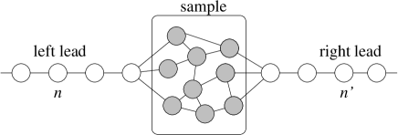
Figure 1: Schematic picture of the system described by Hamiltonian (1).

In this Section we introduce a general Hamiltonian describing a mesoscopic sample coupled to leads as shown in Fig. 1. The Hamiltonian is a generalization of the well known Anderson impurity model Anderson61 . We split the Hamiltonian into five pieces

$$H=H_{L}+V_{L}+H_{C}+V_{R}+H_{R},$$ (1)

where $H_{C}$ models the central region, $H_{L}$ and $H_{R}$ describe the left and the right lead, and $V_{L}$ and $V_{R}$ are the tunneling couplings between the leads and the central region. We can also split the Hamiltonian into a term $H^{\left(0\right)}$ describing independent electrons and a term $U$ describing the Coulomb interaction between them

$$H=H^{\left(0\right)}+U.$$ (2)

One can often neglect the interaction in the leads and between the sample and the leads. We assume this is the case. Then the central region is the only part of the system where one must take the interaction into account

$$H_{\mathrm{C}}=H_{C}^{\left(0\right)}+U.$$ (3)

Here $H_{C}^{\left(0\right)}$ describes a set of noninteracting levels

$$H_{C}^{\left(0\right)}=\sum_{{{i,j\in C\atop\sigma}}}H_{Cji}^{\left(0\right)}d_{j\sigma}^{\dagger}d_{i\sigma},$$ (4)

where $d_{i\sigma}^{\dagger}$ ($d_{i\sigma}$) creates (destroys) an electron with spin $\sigma$ in the state $i$. The states introduced here can have various physical meanings. They could represent the true single-electron states of the sample, for example different energy levels of a multi-level quantum dot or a molecule. In this case, the matrix $H_{Cji}^{\left(0\right)}$ is diagonal and its elements are the single-electron energies of the system. Another possible interpretation of Hamiltonian (4) is that the states $i$ are local orbitals at different sites of the system. In this case, the diagonal matrix elements of $H_{C}^{\left(0\right)}$ are the on-site energies for these sites, while the off-diagonal matrix elements describe the coupling between different sites of the system. The sites could have a direct physical interpretation, such as dots in a double quantum dot system or atoms in a molecule, or they could represent fictitious sites obtained by discretization of a continuous system. There are other possible choices of basis states for the central region. For example, in a system consisting of two multi-level quantum dots one could use single-electron basis states for each of the dots and describe the coupling between the dots with tunneling matrix elements.

The Coulomb interaction between electrons in the sample is given by an extended Hubbard-type coupling

$$U=\frac{1}{2}\sum_{{{i,j\in C\atop\sigma,\sigma^{\prime}}}}U_{ji}^{\sigma\sigma^{\prime}}n_{j\sigma}n_{i\sigma^{\prime}},$$ (5)

where $n_{i\sigma}=d_{i\sigma}^{\dagger}d_{i\sigma}$ is the operator counting the number of electrons with spin $\sigma$ at site $i$. For convenience, we wrote down only the expression for the Coulomb interaction in the case, where basis states represent different sites in real space. The expression becomes more complicated if a more general basis set is used.

We describe the leads or contacts as two semi-infinite, tight-binding chains

$$H_{\mathrm{L}\left(R\right)}=-t_{0}\sum_{{{i,i+1\in L\left(R\right)\atop\sigma}}}c_{i\sigma}^{\dagger}c_{i+1\sigma}+\mathrm{h.c.},$$ (6)

where $c_{i\sigma}^{\dagger}$ ($c_{i\sigma}$) creates (destroys) an electron with spin $\sigma$ on site $i$ and $t_{0}$ is the hopping matrix element between neighboring sites. Such a model adequately, at least for energies low or comparable to $t_{0}$, describes a noninteracting, single-mode and homogeneous lead. It would be easy to generalize the lead Hamiltonian to describe a more realistic system, for example by modeling the true geometry or allowing for a self-consistent potential due to interaction between electrons. However, the physics we are interested in, is usually not changed dramatically by not including these details into the model Hamiltonian and therefore, we will not discuss this issue into detail.

Finally, there is a term describing the coupling between the sample and the leads,

$$V_{L\left(R\right)}=\sum_{{{j\in L\left(R\right)\atop{{i\in C\atop\sigma}}}}}V_{L\left(R\right)ji}c_{j\sigma}^{\dagger}d_{i\sigma}+\mathrm{h}.\mathrm{c}.,$$ (7)

where $V_{L\left(R\right)ji}$ is the hopping matrix element between state $i$ in the sample and site $j$ in a lead.

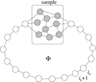
Figure 2: The sample embedded in a ring formed by joining the left and right leads of the system in Fig. 1. Magnetic flux $\Phi$ penetrates the ring.

In the following Sections we discuss the conductance through the system introduced above. To derive the conductance formulae, we will need a slightly modified system. This auxiliary system is a ring formed by connecting the ends of the left and right leads of the original system as shown in Fig. 2. The ring is threaded by a magnetic flux $\Phi$ in such a way that there is no magnetic field in the region where electrons move. We can then perform the standard Peierls substitution Peierls33 and transform the hopping matrix elements of the Hamiltonian (1) according to

$$t_{ji}\rightarrow t_{ji}e^{i\frac{e}{\hbar}\int_{\mathbf{x}_{i}}^{\mathbf{x}_{j}}\mathbf{A}\cdot\mathrm{d}\mathbf{x}},$$ (8)

where $\mathbf{x}_{i}$ is the position of site $i$ and $\mathbf{A}$ is the vector potential due to the flux, obeying

$$\Phi=\frac{\hbar}{e}\phi=\oint\mathbf{A}\cdot\mathrm{d}\mathbf{x}.$$ (9)

Here we defined a dimensionless magnetic flux $\phi$. The energy of the system is periodic in $\phi$ with a period of $2\pi$ and depends only on value of $\phi$ and not on any details of how the flux is produced. If the original Hamiltonian (1) obeys the time-reversal symmetry, the energy does not change if the magnetic field is reversed,

$$E\left(-\phi\right)=E\left(\phi\right).$$ (10)

III Conductance of a noninteracting system

In this Section we limit the discussion to noninteracting systems, i.e. we set $U=0$ in Eq. (2). In such systems, the Landauer-Büttiker formulaLandauer57 ; Landauer70 ; Buttiker86

$$G=G_{0}\left|t\left(\varepsilon_{F}\right)\right|^{2},$$ (11)

which relates the zero-temperature conductance $G$ to the transmission probability $\left|t\left(\varepsilon_{F}\right)\right|^{2}$ for electrons at the Fermi energy $\epsilon_{F}$, can be applied. The proportionality coefficient, $G_{0}=\frac{2e^{2}}{h}$, is the quantum of conductance. Below we first derive a set of formulae, which relate the transmission probability, and consequently the conductance, to single-electron energy levels of the auxiliary ring system introduced in the previous Section. Then we derive another set of formulae, relating the conductance to the ground-state energy of the auxiliary system. One of these formulae was derived before in Ref. Sushkov01 , and a limiting case of another one was discussed in Refs. Favand98 ; Molina02 . Here we present a unified approach to the problem, from which these results emerge as special cases.

III.1 Formulae relating conductance to single-electron energy levels

Let us consider eigenstates of an electron moving on a ring system introduced in the previous Section. We will be interested only in energies of these states and not in the precise form of wavefunctions. The energy of an electron on a ring penetrated by a magnetic flux $\phi$ depends only on the magnitude of the flux and therefore, any vector potential fulfilling condition (9) is good for our purpose. We choose a vector potential constant everywhere except between sites $i_{0}$ and $i_{0}+1$, both in the lead part of the ring as shown in Fig. 2. The hopping matrix element between the two sites is thus modified to $t_{0}e^{i\phi}$. With no flux penetrating the ring, the electron’s wavefunction in the lead part of the system is $ae^{iki}+be^{-iki}$, where $k$ is the electron’s wavevector and $a$ and $b$ are amplitudes determined by properties of the central region. If there is a flux through the ring, the wavefunction is modified. The Schrödinger equations for sites $i_{0}$ and $i_{0}+1$ show us that the appropriate form is $ae^{iki}+be^{-iki}$ for $i\leq i_{0}$ and $ae^{-i\phi}e^{iki}+be^{-i\phi}e^{-iki}$ for $i>i_{0}$. The scattering matrix of the central region provides a relation between coefficients $a$ and $b$,

$$\left(\begin{array}[]{c}be^{-i\phi}e^{ikN}\\ a\end{array}\right)=\left(\begin{array}[]{cc}r_{k}&t_{k}^{\prime}\\ t_{k}&r_{k}^{\prime}\end{array}\right)\left(\begin{array}[]{c}ae^{-i\phi}e^{-ikN}\\ b\end{array}\right).$$ (12)

The elements of the scattering matrix, $t_{k}$ and $r_{k}$ ($t_{k}^{\prime}$ and $r_{k}^{\prime}$), are the transmission and reflection amplitudes for electrons coming from the left (right) lead, and $N$ is the number of sites in the lead part of the ring. We added phase factors $e^{\pm ikN}$ to the “left lead” amplitudes to compensate for the phase difference an electron accumulates as it travels through the lead part of the ring. The scattering matrix defined this way does not depend on $N$ and $\phi$, and equals the scattering matrix of the original, two-lead system. Eq. (12) is a homogeneous system of linear equations, solvable only if the determinant is zero. Using the unitarity property of the scattering matrix, the eigenenergy condition becomes

$$t_{k}^{\prime}e^{i\phi}+t_{k}e^{-i\phi}=e^{ikN}+\frac{t_{k}}{t_{k}^{\prime\ast}}e^{-ikN}.$$ (13)

We assume the Hamiltonian of the original, two lead system obeys the time-reversal symmetry and therefore, the scattering matrix is symmetric Datta95 , $t_{k}=t_{k}^{\prime}$. Expressing the transmission amplitude in terms of its absolute value and the scattering phase shift $t_{k}=\left|t_{k}\right|e^{i\varphi_{k}}$, we arrive at the final form of the eigenenergy equation

$$\left|t_{k}\right|\cos\phi=\cos\left(kN-\varphi_{k}\right).$$ (14)

In Fig. 3 a graphical representation of this equation is presented.

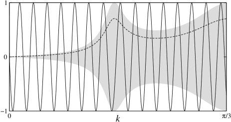
Figure 3: A graphical representation of the eigenvalue equation (14). The shaded region represents the allowed values of the left hand side of the equation for different values of magnetic flux (for example, the dashed line shows the values for $\phi=\frac{\pi}{4}$). The full line represents the right hand side of the eigenvalue equation. The system is presented in Fig. 7, $N=100$.

To extract the transmission probability $\left|t_{k}\right|^{2}$, we proceed by differentiating the eigenvalue equation with respect to $\cos\phi$

$$\frac{\partial\left|t_{k}\right|}{\partial\cos\phi}\cos\phi+\left|t_{k}\right|=$$

$$\quad=-\sin\left(kN+\varphi_{k}\right)\left(N\frac{\partial k}{\partial\cos\phi}+\frac{\partial\varphi_{k}}{\partial\cos\phi}\right)=$$

$$\quad=\pm\sqrt{1-\left|t_{k}\right|^{2}\cos^{2}\phi}\left(N\frac{\partial k}{\partial\cos\phi}+\frac{\partial\varphi_{k}}{\partial\cos\phi}\right).\quad\quad$$ (15)

The sign of the last expression depends on weather $k$ belongs to a decreasing ($+$) or an increasing ($-$) branch of the cosine function in Eq. (14), or equivalently, if we are interested in an eigenstate with odd ($+$) or even ($-$) $n$, where $n$ indexes the eigenstates from the one with the lowest energy upward. Let us choose an eigenstate and consider how the corresponding wavevector $k$ changes as the magnetic flux $\phi$ is varied from 0 to $\pi$. It is evident that the variation in $k$ is of the order of $\frac{1}{N}$ as the cosine function in the right hand side of Eq. (14) oscillates with such a period. Let as assume that the number of sites in the ring is large enough that transmission amplitude does not change appreciably in this interval

$$\left|\frac{\partial t_{k}}{\partial k}\right|\frac{\pi}{N}\ll 1.$$ (16)

Then the derivatives $\frac{\partial k}{\partial\cos\phi}$, $\frac{\partial\left|t_{k}\right|}{\partial\cos\phi}$ and $\frac{\partial\varphi_{k}}{\partial\cos\phi}$ are of the order of $\frac{1}{N}$ and Eq. (15) simplifies to

$$\left|t_{k}\right|=\pm\sqrt{1-\left|t_{k}\right|^{2}\cos^{2}\phi}N\frac{\partial k}{\partial\cos\phi}+\mathcal{O}\left(\frac{1}{N}\right).$$ (17)

Introducing the density of states in the leads $\rho\left(\varepsilon\right)=\frac{1}{\pi}\frac{\partial k}{\partial\varepsilon},$ which for example, for a tight-binding lead with only nearest-neighbor hopping $t_{0}$ and dispersion $\varepsilon_{k}=-2t_{0}\cos k$ equals $1/\bigl{(}\pi\sqrt{4t_{0}^{2}-\varepsilon_{k}^{2}}\bigr{)}$, we finally obtain

$$\frac{\partial\arccos\left(\mp\left|t\left(\varepsilon_{k}\right)\right|\cos\phi\right)}{\partial\cos\phi}=\pi N\rho\left(\varepsilon_{k}\right)\frac{\partial\varepsilon_{k}}{\partial\cos\phi},$$ (18)

where $t\left(\varepsilon_{k}\right)=t_{k}$. The condition Eq. (16) of validity can also be expressed in a form involving energy as a variable

$$N\gg\frac{1}{\rho\left(\varepsilon\right)}\left|\frac{\partial t\left(\varepsilon\right)}{\partial\varepsilon}\right|.$$ (19)

Eq. (18) is the central result of this work. It expresses the transmission probability $\left|t\left(\varepsilon\right)\right|^{2}$ of a sample connected to two leads in terms of the variation of single-electron energy levels with magnetic flux penetrating the auxiliary ring system. Employing the Landauer-Büttiker formula Eq. (11), this result also provides the zero-temperature conductance of the system. From the derivation it is evident that the method becomes exact as we approach the thermodynamic limit $N\to\infty$.

In general Eq. (18) has to be solved numerically to obtain the transmission probability on a discrete set of energy points, one for each energy level of a system. By increasing the system size $N$, the density of these points increases and the errors decrease, as the condition (19) is fulfilled better. We will return to this point in Section V where we consider the convergence issues in detail. Here we present some special cases of Eq. (18) where analytic expressions can be obtained. By averaging the equation over values of flux $\phi$ between $\phi=0$ and $\phi=\pi$ (note that we may treat $\left|t\left(\varepsilon_{k}\right)\right|$ and $\rho\left(\varepsilon_{k}\right)$ as constant while averaging as the resulting error is of the order of $\frac{1}{N}$), we can relate the transmission probability to the average magnitude of the derivative of a single-electron energy with respect to the flux:

$$\left|t\left(\varepsilon_{k}\right)\right|^{2}=\sin^{2}\left(\frac{\pi^{2}}{2}N\rho\left(\varepsilon_{k}\right)\overline{\left|\frac{\partial\varepsilon_{k}}{\partial\phi}\right|}\right).$$ (20)

Note that it is enough to calculate the energy levels at $\phi=0$ and $\phi=\pi$ to calculate the transmission probability as $\overline{\left|\partial\varepsilon_{k}/\partial\phi\right|}=\frac{1}{\pi}\left|\varepsilon_{k}\left(\pi\right)-\varepsilon_{k}\left(0\right)\right|$. In Fig. 4(a) it is illustrated how a large variation of single-electron energy as the flux is changed from $\phi=0$ to $\phi=\pi$ corresponds to a large conductance and vice versa. The transmission probability can also be calculated from the derivative at $\phi=\frac{\pi}{2}$ resulting in the second formula

$$\left|t\left(\varepsilon_{k}\right)\right|^{2}=\left(\pi N\rho\left(\varepsilon_{k}\right)\left.\frac{\partial\varepsilon_{k}}{\partial\phi}\right|_{\phi=\frac{\pi}{2}}\right)^{2}.$$ (21)

Again, Fig. 4(a) shows that there is a correspondence between a large sensitivity of a single-electron energy to the flux at $\phi=\frac{\pi}{2}$, and a large conductance. Finally, we observe that the curvature of energy levels at $\phi=0$ and $\phi=\pi$ also gives information of conductance. The third formula reads

$$\left|t\left(\varepsilon_{k}\right)\right|^{2}=1-\frac{1}{1+\left(\pi N\rho\left(\varepsilon_{k}\right)\left.\frac{\partial^{2}\varepsilon_{k}}{\partial\phi^{2}}\right|_{\phi=0,\pi}\right)^{2}}.$$ (22)

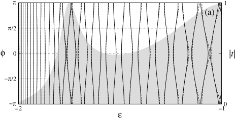
Figure 4: (a) Single-electron energy levels (full lines) and the ground-state energies when a given single-electron level is at the Fermi energy (dashed lines). Ground-state energies are shifted so that both curves coincide for $\phi=\frac{\pi}{2}$. Note that the energy curves are symmetric about $\phi=0$ as required by Eq. (10). The shaded area represents the magnitude of the transmission amplitude. The system and the energy interval is the same as in Fig. 3. (b, c) The large $N$ universal form of the ground-state energy vs. flux curve for an even (b) and an odd (c) number of electrons in a system. The magnitude of the transmission amplitude goes from 0 to 1 in steps of 0.1.

III.2 Formulae relating conductance to the ground-state energy

Above we showed how the flux variation of the energy of the last occupied single-electron state allows one to calculate the zero-temperature conductance through a noninteracting sample. The goal of this section is to derive an alternative set of formulae, expressing the zero-temperature conductance in terms of the flux variation of the ground-state energy $E$, which for an even number of electrons in a noninteracting system is simply a sum of single-electron energies up to the Fermi energy $\varepsilon_{F}$, multiplied by 2 because of the electron’s spin

$$E=2\sum_{\varepsilon_{n}\leq\varepsilon_{F}}\varepsilon_{n}.$$ (23)

We will show that the transmission probability at the Fermi energy $\left|t\left(\varepsilon_{F}\right)\right|^{2}$ is related to the ground-state energy of the ring system

$$\frac{1}{\pi}\frac{\partial\arccos^{2}\left(\mp\left|t\left(\varepsilon_{F}\right)\right|\cos\phi\right)}{\partial\cos\phi}=\pi N\rho\left(\varepsilon_{F}\right)\frac{\partial E}{\partial\cos\phi},$$ (24)

where the sign is $-$ and $+$ for an odd and an even number of occupied single-electron states, respectively. The expression Eq. (24) is evidently correct if there are no electrons in the system, as it gives a zero conductance in this case. To prove the formula for other values of the Fermi energy, we use the principle of the mathematical induction. To simplify the notation we introduce

$$f_{s}\left(\varepsilon_{n}\right)=N\frac{\partial\varepsilon_{n}}{\partial\cos\phi}=\frac{1}{\pi\rho\left(\varepsilon_{n}\right)}\frac{\partial\arccos\left(s\left|t\left(\varepsilon_{n}\right)\right|\cos\phi\right)}{\partial\cos\phi},$$ (25)

$$F_{s}\left(\varepsilon_{n}\right)=N\frac{\partial E_{n}}{\partial\cos\phi}=\frac{1}{\pi^{2}\rho\left(\varepsilon_{n}\right)}\frac{\partial\arccos^{2}\left(s\left|t\left(\varepsilon_{n}\right)\right|\cos\phi\right)}{\partial\cos\phi},$$ (26)

where $E_{n}$ is the ground-state energy of a system with the Fermi energy at $\varepsilon_{n}$ and $s$ is either $1$ or $-1$, depending on the signs in Eqs. (18) and (24). Differentiating the relation $E_{n}=E_{n-1}+2\varepsilon_{n}$ with respect to $\cos\phi$, expressing the result in terms of functions $f_{s}$ and $F_{s}$ introduced above, and making use of the fact that the sign $s$ alternates with $n$, we obtain

$$F_{s}\left(\varepsilon_{n}\right)=F_{-s}\left(\varepsilon_{n-1}\right)+2f_{s}\left(\varepsilon_{n}\right).$$ (27)

If we manage to show that this really is an identity, we have a proof of Eq. (24). Using the exact relation $F_{s}\left(\varepsilon\right)-F_{-s}\left(\varepsilon\right)=2f_{s}\left(\varepsilon\right)$, the expression transforms into

$$F_{s}\left(\varepsilon_{n}\right)=F_{s}\left(\varepsilon_{n}\right)-\left[F_{-s}\left(\varepsilon_{n}\right)-F_{-s}\left(\varepsilon_{n-1}\right)\right].$$ (28)

For a large number of sites $N$ in the ring and correspondingly, a small separation of single-electron energy levels which is of the order of $\frac{1}{N}$, the term in parenthesis equals $F_{-s}^{\prime}\left(\varepsilon_{n}\right)\left(\varepsilon_{n}-\varepsilon_{n-1}\right)$. $F_{-s}^{\prime}\left(\varepsilon_{n}\right)$ can be factored into $s\tilde{F}\left(\varepsilon_{n}\right)$ where $\tilde{F}\left(\varepsilon_{n}\right)$ does not depend on sign $s$. Therefore, although the term in parenthesis in of the order of $\frac{1}{N}$, its sign alternates for successive energy levels while its amplitude stays the same. Thus the error induced by this term does not accumulate, it just adds an additional error of the order of $\frac{1}{N}$ to the final result.

In Fig. 4(a), the variation of the ground-state energies with magnetic flux is compared to the variation of the corresponding single-electron energies. Note that as a consequence of Eq. (24), the ground-state energy in the large $N$ limit takes a universal form (see Fig. 4(b))

$$\!\!\!\!\!\!E\left(\phi\right)-E\left(\frac{\pi}{2}\right)=$$

$$\!\!\!\!\!\!\quad=\frac{1}{\pi^{2}N\rho\left(\varepsilon_{F}\right)}\Bigl{(}\arccos^{2}\left(\mp\left|t\left(\varepsilon_{F}\right)\right|\cos\phi\right)-\frac{\pi^{2}}{4}\Bigr{)}.\quad\quad$$ (29)

For systems with an odd number of electrons, the ground-state energy is obtained by adding a single-electron energy corresponding to Eq. (18) and the universal form reads (see Fig. 4(c))

$$E\left(\phi\right)-E\left(\frac{\pi}{2}\right)=\frac{1}{\pi^{2}N\rho\left(\varepsilon_{F}\right)}\arcsin^{2}\left(\left|t\left(\varepsilon_{F}\right)\right|\cos\phi\right).$$ (30)

In general, Eq. (24) can only be solved numerically to obtain the transmission probability. However, as was the case for single-electron energies, analytic solutions can be found in certain special cases. The derivative of the ground-state energy with respect to flux gives the persistent current in the ring $j=\frac{e}{\hbar}\frac{\partial E}{\partial\phi}$ Bloch65 ; Buttiker83 . Using the Landauer-Büttiker formula Eq. (11), one can calculate the conductance from the flux averaged magnitude of the persistent current in the system

$$\left|t\left(\varepsilon_{F}\right)\right|^{2}=\sin^{2}\left(\frac{\pi^{2}\hbar}{2e}N\rho\left(\varepsilon_{F}\right)\overline{\left|j\left(\phi\right)\right|}\right).$$ (31)

Only two ground-state energy calculations need to be performed to obtain the conductance as $\frac{\hbar}{e}\overline{\left|j\left(\phi\right)\right|}=\frac{1}{\pi}\left|E\left(\pi\right)-E\left(0\right)\right|$. This formula was also discussed in Refs. Favand98 ; Molina02 for the case where the transmission probability is small. The second formula relates the conductance to the persistent current at $\phi=\frac{\pi}{2}$Sushkov01 ; Meden02 ,

$$\left|t\left(\varepsilon_{F}\right)\right|^{2}=\left(\frac{\pi\hbar}{e}N\rho\left(\varepsilon_{F}\right)j\left(\frac{\pi}{2}\right)\right)^{2}.$$ (32)

The third formula, corresponding to Eq. (22) in the single-electron case, turns out to be more complicated and gives an implicit relation for $\left|t\left(\varepsilon_{F}\right)\right|$

$$\pi N\rho\left(\varepsilon_{F}\right)\left.\frac{\partial^{2}E}{\partial\phi^{2}}\right|_{\mathrm{min,}\,\mathrm{max}}=$$

$$\quad=\pm\frac{2\left|t\left(\varepsilon_{F}\right)\right|}{\pi\sqrt{1-\left|t\left(\varepsilon_{F}\right)\right|^{2}}}\arccos\left(\pm\left|t\left(\varepsilon_{F}\right)\right|\right).$$ (33)

Here the upper and the lower signs correspond to the second derivative at a minimum and at a maximum of the energy vs. flux curve, respectively. Minima (maxima) occur at $\phi=0\left(\pi\right)$ if an odd number of single-electron levels is occupied and at $\phi=\pi\left(0\right)$ if an even number of levels is occupied. The second derivative in a minimum is proportional to the charge stiffness $D=\frac{N}{2}\left.\partial^{2}E/\partial\phi^{2}\right|_{\mathrm{min}}$ of the systemKohn64 ; Prelovsek01 . We can also define the corresponding quantity for a maximum as $\tilde{D}=-\frac{N}{2}\left.\partial^{2}E/\partial\phi^{2}\right|_{\mathrm{max}}$. In general, Eq. (33) has to be solved numerically. However, in the limit of a very small conductance and in the vicinity of the unitary limit, additional analytic formulae are valid

$$\left|t\left(\varepsilon_{F}\right)\right|=\left\{\begin{array}[]{ll}2\pi\rho\left(\varepsilon_{F}\right)D,&\left|t\left(\varepsilon_{F}\right)\right|\rightarrow 0,\\ \frac{1}{2}+\frac{3\pi}{4}2\pi\rho\left(\varepsilon_{F}\right)D,&\left|t\left(\varepsilon_{F}\right)\right|\rightarrow 1.\end{array}\right.$$ (34)

Note that there is a quadratic relation between the conductance and the charge stiffness in the low conductance limit. The corresponding formulae for the maximum of the energy vs. flux curve are

$$\left|t\left(\varepsilon_{F}\right)\right|=\left\{\begin{array}[]{ll}2\pi\rho\left(\varepsilon_{F}\right)\tilde{D},&\left|t\left(\varepsilon_{F}\right)\right|\rightarrow 0,\\ 1-\frac{2}{\left(2\pi\rho\left(\varepsilon_{F}\right)\tilde{D}\right)^{2}},&\left|t\left(\varepsilon_{F}\right)\right|\rightarrow 1.\end{array}\right.$$ (35)

A detailed analysis of convergence properties of the formulae derived in this Section is presented Section V.

We stress again that the validity of these formulae is based on an assumption that the number of sites in the ring is sufficiently large according to the condition Eq. (19). This means that if $t(\varepsilon)$ exhibits sharp resonances, the calculation has to be performed on such a large auxiliary ring system that in the energy interval of interest (the width of the resonance) there is a large number of eigenenergies $\varepsilon_{n}$. Then $t(\varepsilon)\sim t(\varepsilon_{n^{\prime}})$, where $\varepsilon_{n^{\prime}}$ is the eigenenergy closest to $\varepsilon$. Such sharp resonances in $t(\varepsilon)$ are expected e.g. in chaotic systems Jalabert92 ; Verges98 . The present method might be impractical (but still correct) in this case.

IV Conductance of an interacting system

The zero-temperature conductance of a noninteracting system can thus be determined with the transmission probability obtained from one of the formulae we derived in the previous Section, and the Landauer-Büttiker formula. The main challenge, however, remains the question of the validity of this type of approach for interacting systems. In this Section we give arguments why the approach is correct for a class of interacting systems exhibiting Fermi liquid properties. In order to reach this goal, we present four essential steps as follows.

Step 1: Conductance of a Fermi liquid system at $\bm{T}\bm{=}\bm{0}$

The basic property that characterizes Fermi liquid systemsNozieres64 is that the states of a noninteracting system of electrons are continuously transformed into states of the interacting system as the interaction strength increases from zero to its actual value. One can then study the properties of such a system by means of the perturbation theory, regarding the interaction strength as the perturbation parameter. The concept of the Fermi liquid was first introduced for translation-invariant systems by LandauLandau56 ; Landau57 , and was later also extended to systems of the type we study hereNozieres74 .

The linear response conductance of a general interacting system of the type shown in Fig. 1 can be calculated from the Kubo formula Bruus02 ; Oguri01

$$G=\lim_{\omega\rightarrow 0}\frac{ie^{2}}{\omega+i\delta}\Pi_{II}\left(\omega+i\delta\right),$$ (36)

where $\Pi_{II}\left(\omega+i\delta\right)$ is the retarded current-current correlation function

$$\Pi_{II}\left(t-t^{\prime}\right)=-i\theta\left(t-t^{\prime}\right)\left\langle\left[I\left(t\right),I\left(t^{\prime}\right)\right]\right\rangle.$$ (37)

For Fermi liquid systems at $T=0$, the current-current correlation function can be expressed in terms of the Green’s function $G_{n^{\prime}n}\left(z\right)$ of the system and the conductance is given with Oguri01

$$G=\frac{2e^{2}}{h}\left|\frac{1}{-i\pi\rho\left(\varepsilon_{F}\right)}e^{-ik_{F}\left(n^{\prime}-n^{\prime}\right)}G_{n^{\prime}n}\left(\varepsilon_{F}+i\delta\right)\right|^{2},$$ (38)

where $n$ and $n^{\prime}$ are sites in the left and the right lead, respectively. One can define the transmission amplitude as

$$t\left(\varepsilon\right)\equiv\frac{1}{-i\pi\rho\left(\varepsilon\right)}e^{-ik\left(n^{\prime}-n\right)}G_{n^{\prime}n}\left(\varepsilon+i\delta\right),$$ (39)

and the conductance formula Eq. (38) then reads

$$G=\frac{2e^{2}}{h}\left|t\left(\varepsilon_{F}\right)\right|^{2}.$$ (40)

For non-interacting systems, $t\left(\varepsilon\right)$ defined this way reduces to the standard transmission amplitude (Fisher-Lee relation Fisher81 ) and Eq. (40) represents the Landauer-Büttiker formula. In the next step, we will show that the transmission amplitude Eq. (39) has a direct physical interpretation also for interacting systems, being the transmission amplitude of Fermi liquid quasiparticles.

Step 2: Quasiparticle Hamiltonian

In this step, we generalize the quasiparticle approximation to the Green’s function, presented for the single-impurity Anderson model in Ref. Hewson93 , to the case where the interaction is present in more than a single site.

In Fermi liquid systems obeying the time-reversal symmetry, the imaginary part of the retarded self-energy at $T=0$ vanishes at the Fermi energy and is quadratic for frequencies close to the Fermi energyYamada86 ; Oguri97 . Using the Fermi energy as the origin of the energy scale, i.e. $\omega-\varepsilon_{F}\rightarrow\omega$, we can express this as

$$\mathrm{Im}\bm{\Sigma}\left(\omega+i\delta\right)\propto\omega^{2}.$$ (41)

Close to the Fermi energy, the self-energy can be expanded in powers of $\omega$ resulting in an approximation to the Green’s function,

$$\mathbf{G}^{-1}\left(\omega+i\delta\right)=\omega\mathbf{1}-\mathbf{H}^{\left(0\right)}-\bm{\Sigma}\left(0+i\delta\right)-$$ (42)

$$\quad-\omega\left.\frac{\partial\bm{\Sigma}\left(\omega+i\delta\right)}{\partial\omega}\right|_{\omega=0}+\mathcal{O}\left(\omega^{2}\right).$$ (43)

Here $\mathbf{H}^{\left(0\right)}$ contains matrix elements of the noninteracting part of the Hamiltonian (2). Note that expansion coefficients are real because of Eq. (41). Let us introduce the renormalization factor matrix $\mathbf{Z}$ as

$$\mathbf{Z}^{-1}=\mathbf{1}-\left.\frac{\partial\bm{\Sigma}\left(\omega+i\delta\right)}{\partial\omega}\right|_{\omega=0}.$$ (44)

The Green’s function for $\omega$ close to the Fermi energy can then be expressed as

$$\mathbf{G}^{-1}\left(\omega+i\delta\right)=\mathbf{Z}^{-1/2}\tilde{\mathbf{G}}^{-1}\left(\omega+i\delta\right)\mathbf{Z}^{-1/2}+\mathcal{O}\left(\omega^{2}\right)\!,\!\!$$ (45)

where we defined the quasiparticle Green’s function

$$\tilde{\mathbf{G}}^{-1}\left(\omega+i\delta\right)=\omega\mathbf{1}-\tilde{\mathbf{H}}$$ (46)

as the Green’s function of a noninteracting quasiparticle Hamiltonian

$$\tilde{\mathbf{H}}=\mathbf{Z}^{1/2}\left[\mathbf{H}^{\left(0\right)}+\bm{\Sigma}\left(0+i\delta\right)\right]\mathbf{Z}^{1/2}.$$ (47)

Note that factoring the renormalization factor matrix as we did above ensures the hermiticity of the resulting quasiparticle Hamiltonian.

Matrix elements of $\mathbf{Z}$ differ from those of an identity matrix only if they correspond to sites of the central region. In other cases, as the interaction is limited to the central region, the corresponding self-energy matrix element is zero. Therefore, comparing the quasiparticle Hamiltonian to the noninteracting part of the real Hamiltonian, we observe that the effect of the interaction is to renormalize the matrix elements of the central region Hamiltonian (4) and those corresponding to the hopping between the central region and the leads (7). The values of the renormalized matrix elements depend on the value of the Fermi energy of the system.

Let us illustrate the ideas introduced above for the case of the standard Anderson impurity model Hewson93 . We calculated the self-energy in the second-order perturbation theory approximation Horvatic80 ; Horvatic85 ; Horvatic87 and constructed the quasiparticle Hamiltonian according to Eq. (47). In Fig. 5 the local spectral functions corresponding to both the original interacting Hamiltonian and the noninteracting quasiparticle Hamiltonian are presented. The agreement of both results is perfect in the vicinity of the Fermi energy where the expansion (42) is valid.

Figure 5: The $T=0$ local spectral function and the corresponding quasiparticle approximation for the Anderson impurity model as shown in Fig. 9. The values of parameters are $t_{1}=0.4t_{0}$, $U=1.92t_{0}$ and $\varepsilon_{d}=-\frac{U}{2}$. The calculations were performed within the second-order perturbation theory as described in Appendix A.

The reason for introducing the quasiparticle Hamiltonian is to obtain an alternative expression for the conductance in terms of the quasiparticle Green’s function. Eq. (45) relates the values of the true and the quasiparticle Green’s function at the Fermi energy,

$$\mathbf{G}\left(0+i\delta\right)=\mathbf{Z}^{1/2}\tilde{\mathbf{G}}\left(0+i\delta\right)\mathbf{Z}^{1/2}.$$ (48)

Specifically, if both $n$ and $n^{\prime}$ are sites in the leads, $G_{n^{\prime}n}\left(0+i\delta\right)=\tilde{G}_{n^{\prime}n}\left(0+i\delta\right)$ as a consequence of the properties of the renormalization factor matrix $\mathbf{Z}$ discussed above. Eq. (39) then tells us that the zero-temperature conductance of a Fermi liquid system is identical to the zero-temperature conductance of a noninteracting system defined with the quasiparticle Hamiltonian for a given value of the Fermi energy.

Step 3: Quasiparticles in a finite system

The conclusions reached in the first two steps are based on an assumption of the thermodynamic limit, i.e. they are valid if the central region is coupled to semiinfinite leads. Here we generalize the concept of quasiparticles to a finite ring system with $N$ sites and $M$ electrons, threaded by a magnetic flux $\phi$. Let us define the quasiparticle Hamiltonian for such a system,

$$\tilde{\mathbf{H}}\left(N,\phi;M\right)=\mathbf{Z}^{1/2}\left[\mathbf{H}^{\left(0\right)}\left(N,\phi\right)+\bm{\Sigma}\left(0+i\delta\right)\right]\mathbf{Z}^{1/2}.$$ (49)

Here the self-energy and the renormalization factor matrix are determined in the thermodynamic limit where, as we prove in Appendix A, they are independent of $\phi$ and correspond to those of an infinite two-lead system.

Suppose now that we knew the exact values of the renormalized matrix elements in the quasiparticle Hamiltonian (49). As this is a noninteracting Hamiltonian, we could then apply the conductance formulae of the previous Section to calculate the zero-temperature conductance of an infinite two-lead system with the same central region and central region-lead hopping matrix elements, i.e. of a system described with the quasiparticle Hamiltonian (47). As shown in step 2, this procedure would provide us with the exact conductance of the original interacting system. However, to obtain the values of the renormalized matrix elements, one needs to calculate the self-energy of the system, which is a difficult many-body problem. In the next step, we will show, that there is an alternative and easier way to achieve the same goal.

In Fig. 6 we compare the spectral density of an Anderson impurity embedded in a finite ring system to that of the corresponding quasiparticle Hamiltonian (49). Note that the spectral density of the quasiparticle Hamiltonian correctly describes the true spectral density in the vicinity of the Fermi energy.

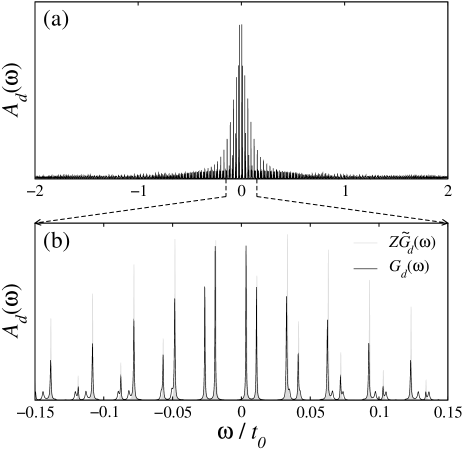
Figure 6: (a) The $T=0$ local spectral function as in Fig. 5, but for a ring system with $N=400$ sites and flux $\phi=\frac{3\pi}{4}$. (b) The spectral function in the vicinity of the Fermi energy (dashed lines) compared to that corresponding to the quasiparticle Hamiltonian (49). Both the spectral density of the interacting system and the matrix elements of the quasiparticle Hamiltonian were calculated within the second order perturbation theory.

Step 4: Validity of the conductance formulae

In this last step we finally show how to calculate the conductance of an interacting system. In Appendix A we study the excitation spectrum of a finite ring system threaded with a magnetic flux and containing a region with interaction. We show that

$$E\left[N,\phi;M+1\right]-E\left[N,\phi;M\right]=$$

$$\quad=\tilde{\varepsilon}\left(N,\phi;M;1\right)+\mathcal{O}\left(N^{-\frac{3}{2}}\right),$$ (50)

where $E\left(N,\phi;M\right)$ and $E\left(N,\phi;M+1\right)$ are the ground-state energies of the interacting Hamiltonian for a ring system with $N$ sites and flux $\phi$, containing $M$ and $M+1$ electrons, respectively, and $\tilde{\varepsilon}\left(N,\phi;M;1\right)$ is the energy of the first single-electron level above the Fermi energy of the finite ring quasiparticle Hamiltonian (49). This estimation allows one to use single-electron formulae of Sec. III.1 to calculate the zero-temperature conductance for a Fermi liquid system. We showed in step 3 that inserting $\tilde{\varepsilon}\left(N,\phi;M;1\right)$ into these formulae would give us the correct conductance. Eq. (50) proves, that the same result is obtained if the difference of the ground state energies of an interacting system $E\left[N,\phi;M+1\right]-E\left[N,\phi;M\right]$ is inserted into a formula instead. The estimated error, which is of the order of $N^{-\frac{3}{2}}$, is for a large $N$ negligible, because it is much smaller than the quasiparticle level spacing, which is of the order of $\frac{1}{N}$.

As demonstrated in Sec. III.2, the conductance of a noninteracting system can also be calculated from the variation of the ground-state energy with flux through the ring. The proof of the formulae involved only the properties of a set of neighboring single-electron energy levels. We assumed the validity of single-electron conductance formulae for each of these levels and made use of the fact that the ground-state energy of the system increases by a sum of the relevant single-electron energies as the levels become occupied with additional electrons. For Fermi liquid systems, the first assumption was proved above. The second assumption, which for noninteracting systems is obvious, is proved in Appendix A. There we show that as a finite number of additional electrons is added to an interacting system, the successive ground-state energies are determined by the single-electron energy levels of the same quasiparticle Hamiltonian with a very good accuracy (51). Therefore, the proof of Sec. III.2 is also valid for interacting Fermi liquid systems, provided a system is the Fermi liquid for all values of the Fermi energy below its actual value.

V Numerical tests of the method

V.1 Noninteracting system

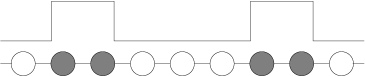
Figure 7: A double barrier noninteracting system. The height of the barriers is $0.5t_{0}$, where $t_{0}$ is the hopping matrix element between neighboring sites.

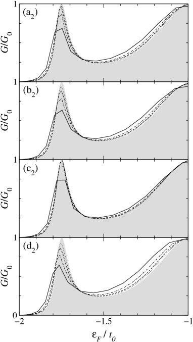
Figure 8: Exact and approximate zero-temperature conductance vs. Fermi energy curves for the system in Fig. 7. The shaded area shows the exact result. The left set of figures shows the approximations obtained using the single-electron formulae of Sec. III.1 while the right set of figures corresponds to the ground-state energy formulae of Sec. III.2. Different curves correspond to different number of sites $N$ in the ring. In figures ($\mathrm{a}_{1}$) and ($\mathrm{a}_{2}$) the conductance was calculated using Eqs. (20) and (31), in figures ($\mathrm{b}_{1}$) and ($\mathrm{b}_{2}$) using Eqs. (21) and (32), while in the other figures Eqs. (22) and (33) were used, in ($\mathrm{c}_{1}$) and ($\mathrm{c}_{2}$) applied to the maximum and in ($\mathrm{d}_{1}$) and ($\mathrm{d}_{2}$) to the minimum of energy vs. flux curves.

In this Section we discuss the convergence properties of the conductance formulae derived in Sec. III. As a test system we use a double-barrier potential scattering problem presented in Fig. 7. Results of various formulae for different number of sites in the ring are presented in Fig. 8. The exact zero-temperature conductance for this system exhibits a sharp resonance peak superimposed on a smooth background conductance. We notice immediately that as the number of sites in the ring increases, the convergence is generally faster in the region where the conductance is smooth than in the resonance region, which is consistent with the condition (19). Comparing the results obtained employing different conductance formulae we observe that the convergence is the fastest in both the single-electron and the ground-state energy case if the formulae of Eqs. (22) and (33) are applied to the maximum of the energy vs. flux curve (or to the minimum in the single-electron case). Formulae of Eqs. (20) and (31) expressing the conductance in terms of the difference of the energies at $\phi=0$ and $\phi=\pi$ converge somewhat slower. Note however that in the former case the second derivative of the energy with respect to the flux has to be evaluated while in the later, the energy difference is large and because of that, the calculation is much more well behaved. From the computational point of view there is another advantage of the energy difference formulae. In this case, all the matrix elements can be made real if one chooses such a vector potential that only one hopping matrix element if modified by the flux as then the additional phase factor is $e^{\pm i\pi}=-1$. Finally, the remaining formulae, employing the slope of the energy vs. flux curve at $\phi=\frac{\pi}{2}$ and the curvature in the minimum of the ground-state energy vs. flux curve, do not show convergence properties comparable to those of the formulae discussed above.

V.2 Anderson impurity model

In 1980s several theories Glazman88 ; Ng88 were put forward proposing a realization of the Anderson impurity model Anderson61 in systems consisting of a quantum dot coupled to two leads (see Fig. 9). These theories show that the topmost occupied energy level in a quantum dot with an odd number of electrons can be associated with the Anderson model $\varepsilon_{d}$ level and such a system should mimic the old Kondo problem of a magnetic spin $\frac{1}{2}$ impurity in a metal host. In recent years signatures of the Kondo physics in electron transport through quantum dots have also been found experimentally Goldhaber98 ; Wiel00 . The Anderson model is well defined and is an attractive testing ground for new numerical and analytical methods that are developed to tackle other challenging many-body problems. Therefore, we will also take it as a nontrivial example to test results of the conductance formulae we derived in this paper.

Figure 9: The Anderson impurity model realized as a quantum dot coupled to two leads. The dot is described with the energy level $\varepsilon_{d}$ and the Coulomb energy of a doubly occupied level $U$. $t_{1}$ is the hopping between the dot and leads.

There are three distinct parameter regimes of the Anderson model. If $\varepsilon_{d}<\varepsilon_{F}<\varepsilon_{d}+U$ with $\left|\varepsilon_{d}+U-\varepsilon_{F}\right|\gg\Delta$ and $\left|\varepsilon_{d}-\varepsilon_{F}\right|\gg\Delta$, where $\Delta$ is the coupling of the quantum dot to leads, we are in the Kondo regime. In this regime, a narrow Kondo resonance is formed in the spectral function at the Fermi energy for temperatures below and close to the Kondo temperature, which corresponds to the width of the resonance. The zero-temperature conductance in the Kondo regime reaches the unitary limit of $\frac{2e^{2}}{h}$. Letting either $\varepsilon_{d}$ or $\varepsilon_{d}+U$ approach the Fermi energy so that $\left|\varepsilon_{d}+U-\varepsilon_{F}\right|$ or $\left|\varepsilon_{d}-\varepsilon_{F}\right|$ becomes comparable with $\Delta$, we enter the mixed valence regime where the charge fluctuations on the dot become important. In this regime, the resonance becomes wider and merges with the resonance corresponding to $\varepsilon_{d}$ or $\varepsilon_{d}+U$ levels. More important for our discussion is the fact that the resonance moves away from the Fermi energy and therefore, the conductance drops as we enter this regime. Finally, there are two nonmagnetic regimes, one in which the “impurity” level is predominately empty, $\varepsilon_{d}-\varepsilon_{F}\gg\Delta$, known as the empty orbital regime, and the corresponding regime where the dot is doubly occupied. In these regimes, the conductance drops toward zero.

In Fig. 10 the zero-temperature conductance through a quantum dot acting as an Anderson impurity is presented and compared to exact results of the Bethe ansatz approachWiegman82a ; Wiegman83 . To calculate the conductance, Eq. (31) was used, with the ground-state energies at $\phi=0$ and $\phi=\pi$ obtained using the variational method presented in Appendix B. There are two variational parameters defining the auxiliary Hamiltonian (70), one describing the effective energy level on the dot and the other renormalizing hoppings into the leads. Two different variational basis sets were used in calculations. In the first set, the basis consisted of wavefunctions (71). As a result of the rotational symmetry in the spin degree of freedom, two of the basis functions may be merged into one. Therefore, the basis set consisted of projections of the auxiliary Hamiltonian ground state $\left|\tilde{0}\right\rangle$ to states with empty $P_{0}\left|\tilde{0}\right\rangle$, singly occupied $P_{1}\left|\tilde{0}\right\rangle=P_{\uparrow}\left|\tilde{0}\right\rangle+P_{\downarrow}\left|\tilde{0}\right\rangle$ and doubly occupied $P_{2}\left|\tilde{0}\right\rangle$ dot level. In the second basis set, wavefunctions $P_{1}VP_{0}\left|\tilde{0}\right\rangle,$ $P_{0}VP_{1}\left|\tilde{0}\right\rangle$, $P_{2}VP_{1}\left|\tilde{0}\right\rangle$ and $P_{1}VP_{2}\left|\tilde{0}\right\rangle$ (76) were added to those of the first set, with $V=V_{L}+V_{R}$ being the operator describing the hopping between the dot and the leads (7). For each position of the $\varepsilon_{d}$ level relative to the Fermi energy, we increased the number of sites in the ring until the conductance converged. The number of sites needed to achieve convergence (see Fig. 11a) was the lowest in the empty orbital regime and the highest (about 1000 for the system shown in Fig. 10) in the Kondo regime. This is a consequence of Eq. (19) as a narrow resonance related to the Kondo resonance appears in the transmission probability of the quasiparticle Hamiltonian (47) in the Kondo regime. In the mixed valence regime, the width of the resonance becomes comparable to $\Delta$, which is much larger than the Kondo temperature and the convergence is thus faster. In the empty orbital regime the resonance moves away from the Fermi energy and an even smaller number of sites is needed to achieve convergence.

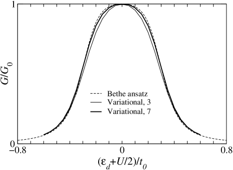
Figure 10: The zero-temperature conductance calculated from ground-state energy vs. magnetic flux in a finite ring system using the variational method of Appendix B with 3 and 7 basis functions. For comparison, the exact Bethe ansatz result is presented with a dashed line. The system shown in Fig. 9 was used, with $U=0.64t_{0}$ and $t_{1}=0.2t_{0}$.

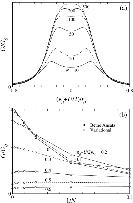
Figure 11: (a) Results of conductance calculations using Eq. (31) for the system presented in Fig. 10 as the number of sites in the ring increases. Note that the convergence is the fastest in the empty orbital regime and the slowest in the Kondo regime. (b) Finite-size scaling analysis of the same results for various values of $\varepsilon_{d}$. With black dots, the Bethe ansatz values are shown. Energies were calculated using the variational method of Appendix B with 7 variational basis functions.

Let us return to results shown in Fig. 10. Note that extending the variational space from 3 to 7 basis functions significantly improves the agreement with the exact result. The remaining discrepancy at the larger basis set can be attributed to the approximate nature of the variational method. Another source of error could be the fact that the Bethe ansatz solution assumes there is a constant coupling to an infinitely wide conduction band. In our case, the conduction band is formed by the states in a tight-binding ring, the coupling to which is not constant. However, it is almost constant in the energy interval we are interested in, i.e. near the center of the band. In order to estimate the effect of the nonconstant coupling on the conductance, we calculated the dot occupation number within the second order perturbation theory for both the case of a constant coupling and for the case of a tight-binding ring. We then calculated the conductance in each case making use of the Friedel sum rule Langreth66 . The agreement is significantly better than the difference between the Bethe ansatz and variational conductance curves in Fig. 10. Therefore, we believe that the use of Bethe ansatz results is justified for this particular problem.

In Fig. 11b a finite-size scaling analysis of the convergence is presented. Note that for rings with a large number of sites $N$, the error scales approximately as $\frac{1}{N}$.

V.3 Double quantum dot

The next logical step after studying individual quantum dots is to consider systems of more than one dot. Single quantum dots are often regarded as artificial atoms because of a similar electronic structure and comparable number of electrons in them. By coupling several quantum dots one is thus creating artificial molecules. Here we will not go into detail in describing the physics of such systems. Our goal is to compare results of our conductance formulae to results of other methods for a double quantum dot system presented in Fig. 12.

In the calculation we again employed the conductance formula (31) and calculated the ground-state energies with the variational approach of Appendix B with the variational basis set (71). In Fig. 13 the zero-temperature conductance for the case where the inter-dot and the on-site Coulomb repulsions $V$ and $U$ are of the same size, are plotted as a function of the position of dot energy levels relative to the Fermi energy for various values of the inter-dot hopping matrix element $t_{2}$. The same problem in the particle-hole symmetric case $\varepsilon_{d}+\frac{U}{2}+V=0$ was studied recently in Ref. Oguri97a . The Matsubara Green’s function was calculated with the quantum Monte Carlo method and the values on discrete frequencies were extrapolated to obtain the retarded Green’s function at the Fermi energy. Then Eqs. (40) and (39) were used to calculate the zero-temperature conductance. The results are presented in Fig. 14, together with the conductance calculated within the Hartree-Fock approximation and results of our method. The agreement with the QMC results is excellent, while the Hartree-Fock approximation gives a qualitatively wrong conductance curve, especially at low values of the inter-dot coupling, indicating strong electron-electron correlations in the system. The results of our method for lower values of $V$ are also shown in Fig. 14.

Figure 12: A double quantum dot system. Each of the dots with energy level $\varepsilon_{d}$ and on-site Coulomb repulsion $U$ is coupled to a lead with a hopping matrix element $t_{1}$. The inter-dot hopping $t_{2}$ is also present as is the inter-dot Coulomb repulsion $V$.

Figure 13: The zero-temperature conductance of the system in Fig. 12 as a function of the position of the dot energy level $\varepsilon_{d}$ and inter-dot hopping matrix element $t_{2}$. The remaining parameters are $U=V=t_{0}$ and $t_{1}=0.5t_{0}$.

Figure 14: The zero-temperature conductance of the double quantum dot system of Fig. 12 at $\varepsilon_{d}+\frac{U}{2}+V=0$ as a function of the inter-dot hopping matrix element $t_{2}$ for various values of the inter-dot Coulomb interaction $V$. As a comparison, the Hartree-Fock and quantum Monte Carlo results Oguri97a are presented for $V/t_{0}=1$. Other parameters are the same as in Fig. 13.

VI Summary and Conclusions

We have demonstrated how the zero-temperature conductance of a sample with electron-electron correlations and connected between noninteracting leads can be determined. The method is extremely simple and is based on several formulae connecting the conductance to persistent currents in an auxiliary ring system. The conductance is determined only from the ground-state energy of an interacting system, while in more traditional approaches, one needs to know the Green’s function of the system. The Green’s function approaches are often much more general, allowing the treatment of transport at finite temperatures and for a finite source-drain voltage applied across the sample, which in our method is not possible. However, the advantage of the present method comes from the fact that the ground-state energy is often relatively simple to obtain by various numerical approaches, including variational methods, and could therefore, for zero-temperature problems, be more appropriate.

Let us summarize the key points of the method:

(1) The “open” problem of the conductance through a sample coupled to semiinfinite leads is mapped on to a ”closed” problem, namely a ring threaded by a magnetic flux and containing the same correlated electron region.

(2) For a noninteracting sample, it is shown that the zero-temperature conductance can be deduced from the variation of the energy of the single-electron level at the Fermi energy with the flux in a large, but finite ring system. The conductance is given with Eq. (18), or with three simple formulae Eq. (20), Eq. (21) and Eq. (22).

(3) Alternatively, the conductance of a noninteracting system is expressed in terms of the variation of the ground-state energy with flux, Eq. (24). Three additional conductance formulae, Eq. (31), Eq. (32) and Eq. (33), are derived.

(4) The method is primarily applicable to correlated systems exhibiting Fermi liquid properties at zero temperature. In order to prove the validity of the method for such systems, the concept of Fermi liquid quasiparticles is extended to finite, but large systems. The conductance formulae give the conductance of a system of noninteracting quasiparticles, which is equal to the conductance of the original interacting system. We also proved that for such systems, the ground-state energy of a large ring system is a universal function of the magnetic flux, with the conductance being the only parameter [Eqs. (29) and (30)].

(5) The results of our method are compared to results of other approaches for problems such as the transport through single and double quantum dots containing interacting electrons. The comparison shows an excellent quantitative agreement with exact Bethe ansatz results in the single quantum dot case. The results for a double quantum dot system also perfectly match QMC results of Ref. Oguri97a .

(6) One should additionally point out that in the derivation presented in this paper we assumed the interaction in the leads to be absent. It is clear that this assumption is not justified for all systems. The method cannot be directly applied to systems where the interaction in the leads is essential, as are e.g. systems exhibiting Luttinger liquid properties.

(7) The validity of the method is not limited to systems that do not break the time-reversal symmetry. A generalization to systems with a broken time-reversal symmetry, such as Aharonov-Bohm rings coupled to leads, is possible and will be presented elsewhere Rejec03 .

(8) Another important limitation of the present method is the single channel approximation for the leads. It might be possible to extend the applicability of the method to systems with multi-channel leads by studying the influence of several magnetic fluxes that couple differently to separate channels. This way, one might be able to probe individual matrix elements of the scattering matrix and derive conductance formulae relevant for such more complex systems.

Note added. After the present work was completed the authors met R. A. Molina and R. A. Jalabert who reported about their recent unpublished work where an approach similar to our work is presented Molina02 ; Molina03PC .

Appendix A Fermi liquid in a finite system

In Sec. IV we based the proof of the validity of the conductance formulae for Fermi liquid systems on the assumption that

$$E\left(N,\phi;M+m\right)=E\left(N,\phi;M\right)+\quad\quad$$

$$\quad+\sum_{i=1}^{m}\tilde{\varepsilon}\left(N,\phi;M;i\right)+\mathcal{O}\left(N^{-\frac{3}{2}}\right).$$ (51)

Here $E\left(N,\phi;M+m\right)$ and $E\left(N,\phi;M\right)$ are the ground-state energies of an interacting $N$-site ring with flux $\phi$, containing $M+m$ and $M$ electrons, respectively. $\tilde{\varepsilon}\left(N,\phi;M;i\right)$ is a single-electron energy of the ring quasiparticle Hamiltonian $\tilde{H}\left(N,\phi;M\right)$ as defined in Eq. (49), with the Fermi energy corresponding to $M$ electrons in the system. The index $i$ labels successive single-electron energy levels above the Fermi energy. We assume $m$ to be finite and $N$ approaching the thermodynamic limit. In this Appendix we will give arguments showing that the assumption of Eq. (51) is indeed valid. In Sec. 1 we first express the problem in terms of the Green’s function of the system. In Sec. 2 we study the properties of the self-energy due to interaction in finite ring systems and then use this results to complete the proof in Sec. 3.

A.1 Relation to the Green’s function

Assume we manage to prove Eq. (51) for $m=1$, i.e.

$$E\left(N,\phi;M+1\right)=E\left(N,\phi;M\right)+$$

$$\quad+\tilde{\varepsilon}\left(N,\phi;M;1\right)+\mathcal{O}\left(N^{-\frac{3}{2}}\right).$$ (52)

Then we can use the same result to relate the energy of a system with $M+2$ electrons to that with $M+1$ electrons,

$$\!\!\!\!\!\!\!\!\!\!\!\!\!\!\!\!\!\!E\left(N,\phi;M+2\right)=E\left(N,\phi;M\right)+$$

$$\!\!\!\!\!\!\!\!\!\!\!\!\!\!\!\!\!\!\quad+\tilde{\varepsilon}\left(N,\phi;M;1\right)+\tilde{\varepsilon}\left(N,\phi;M+1;1\right)+\mathcal{O}\left(N^{-\frac{3}{2}}\right).$$ (53)

Now the matrix elements of quasiparticle Hamiltonians $\tilde{H}\left(N,\phi;M+1\right)$ and $\tilde{H}\left(N,\phi;M\right)$ differ by an amount of the order of $\frac{1}{N}$. To see this, note that the shift of the Fermi energy as an electron is added to the system is of the order of $\frac{1}{N}$, producing a shift of the same order in the self-energy and it’s derivative at the Fermi energy, which define the quasiparticle Hamiltonian through Eq. (49). As the difference of the Hamiltonians $\Delta\tilde{H}$ is small, we can use the first order perturbation theory,

$$\!\!\!\!\!\!\!\!\!\!\!\!\!\tilde{\varepsilon}\left(N,\phi;M+1;1\right)=$$

$$\!\!\!\!\!\!\!\!\!\!\!\!\!\quad=\tilde{\varepsilon}\left(N,\phi;M;2\right)+\left\langle N,\phi;M;2\left|\Delta\tilde{H}\right|N,\phi;M;2\right\rangle=$$

$$\!\!\!\!\!\!\!\!\!\!\!\!\!\quad=\tilde{\varepsilon}\left(N,\phi;M;2\right)+\mathcal{O}\left(N^{-2}\right).$$ (54)

In the last step we made use of the fact that the quasiparticle Hamiltonians differ only in a finite number of sites in and in the vicinity of the central region, and of the fact that the amplitude of the quasiparticle single-electron wavefunction $\left|N,\phi;M;2\right\rangle$ is of the order of $\frac{1}{\sqrt{N}}$. Thus we have proved Eq. (51) for $m=2$ and using the same procedure, we can extend the proof to any finite $m$.

To complete the proof, we still need to show the validity of Eq. (52). As a first step, consider the Lehmann representation of the zero-temperature central region Green’s function

$$G_{ji}\left(t,t^{\prime}\right)=-i\theta\left(t-t^{\prime}\right)\bigl{<}0\bigl{|}\bigl{[}d_{j}\left(t\right),d_{i}^{\dagger}\left(t^{\prime}\right)\bigr{]}\bigr{|}0\bigr{>}$$ (55)

of a ring system characterized with $N$ and $\phi$, containing $M$ electrons,

$$G_{ji}\left(N,\phi;M;z\right)=$$

$$\quad=\quad\sum_{n}\frac{\bigl{<}0\bigr{|}d_{j}\bigl{|}n\bigr{>}\bigl{<}n\bigr{|}d_{i}^{\dagger}\bigl{|}0\bigr{>}}{z-\left(E_{n}^{M+1}-E_{0}^{M}\right)}+$$

$$\quad\quad+\sum_{n}\frac{\bigl{<}0\bigr{|}d_{i}^{\dagger}\bigl{|}n\bigr{>}\bigl{<}n\bigr{|}d_{j}\bigl{|}0\bigr{>}}{z-\left(E_{0}^{M}-E_{n}^{M-1}\right)}.$$ (56)

The first sum runs over all basis states with $M+1$ electrons, while the second sum runs over the states with $M-1$ electrons. The difference in the ground-state energies of systems with $M+1$ and $M$ electrons is evidently equal to the position of the first $\delta$-peak above the Fermi energy in the spectral density corresponding to the Green’s function. In what follows, we will try to determine the energy of this $\delta$-peak.

A.2 Self-energy due to interaction

To achieve the goal we have set in the previous Section, we first need to study the structure of the self-energy due to interaction in a finite ring with flux. Let us again consider the Lehmann representation (56) and to be specific, limit ourselves to states above the Fermi energy. Introducing $\varphi_{j}^{n}=\left\langle 0\left|d_{j}\right|n\right\rangle$ and $\varepsilon_{n}=E_{n}^{M+1}-E_{n}^{M}$, we can express the Green’s function as

$$G_{ji}\left(N,\phi;M;z\right)=\sum_{n}\frac{\varphi_{j}^{n}\varphi_{i}^{n\ast}}{z-\varepsilon_{n}}.$$ (57)

This expression can also be interpreted as a local Green’s function of a larger noninteracting system, consisting of the central region and a bath of noninteracting energy levels, the number of which is equal to the number of multi-electron states with $M+1$ and $M-1$ electrons of the original interacting system. The self-energy due to “hopping out of the central region”, which includes both the effects of the interaction as well as those due to the hopping into the ring, can then be expressed as

$$\Sigma_{ji}\left(N,\phi;M;z\right)=\sum_{n}\frac{V_{jn}V_{ni}}{z-\varepsilon_{n}},$$ (58)

where $V_{jn}$ are the ”hopping matrix elements” between the central region and the “bath”. Thus we have shown that, as far as the single-electron Green’s function is concerned, the interacting system can be mapped on a larger, but noninteracting system.

To further clarify the concepts introduced above, we calculated the self-energy due to interaction within the second-order perturbation theory. Following the calculations by Horvatić, Šokčević and Zlatić Horvatic80 ; Horvatic85 ; Horvatic87 for the Anderson model, we sum the second order self-energy diagrams shown in Fig. 15, including Hartree and Fock terms into the unperturbed Hamiltonian. A lengthy but straightforward calculation, which we do not repeat here, shows that one can identify the states $n$ of Eq. (58) with three Hartree-Fock single-electron state indices $\mathbf{q}=\left(q_{1},q_{2},q_{3}\right)$ such that $q_{1}$ and $q_{2}$ are above the Fermi energy and $q_{3}$ is below it (or vice versa), and a spin index $s$. The “bath” energy levels

$$\varepsilon_{\mathbf{q}s}=\varepsilon_{q_{1}}+\varepsilon_{q_{2}}-\varepsilon_{q_{3}}$$ (59)

and the “hopping matrix elements” related to the self-energy for electrons with spin $\sigma$

$$V_{j\mathbf{q}s}=\left\{\begin{array}[]{ll}\sum_{k^{\prime}}U_{jk^{\prime}}^{\sigma\bar{\sigma}}\varphi_{j}^{q_{1}}\varphi_{k^{\prime}}^{q_{2}}\varphi_{k^{\prime}}^{q_{3}\ast},&s=\bar{\sigma},\\ \frac{1}{\sqrt{2}}\sum_{k^{\prime}}U_{jk^{\prime}}^{\sigma\sigma}\left[\varphi_{j}^{q_{1}}\varphi_{k^{\prime}}^{q_{2}}-\varphi_{j}^{q_{2}}\varphi_{k^{\prime}}^{q_{1}}\right]\varphi_{k^{\prime}}^{q_{3}\ast},&s=\sigma\end{array}\right.$$ (60)

are then expressed in terms of the Coulomb interaction matrix elements (5), and the Hartree-Fock single-electron energies $\varepsilon_{q}\left(N,\phi;M\right)$ and the corresponding wavefunctions $\left|\varphi^{q}\left(N,\phi;M\right)\right\rangle$. In Fig. 16 the positions of $\delta$-peaks in the imaginary part of the self-energy as a function of magnetic flux through the ring are plotted. Note that as the flux is varied, the positions of the peaks fluctuate by an amount of the order of the single-electron level spacing which is of the order of $\frac{1}{N}$. The weights of the peaks also depend on the flux. A similar behavior is expected if higher order processes are also taken into account.

Figure 15: Second-order self-energy diagrams.

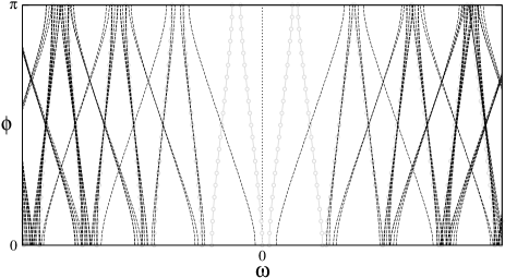
Figure 16: Dashed lines show the positions of $\delta$-peaks (59) in the second-order self-energy corresponding to single-electron energy levels of an unperturbed system presented with gray lines.

Finally, let us study the self-energy in the thermodynamic limit. We will show that in this case, the self-energy is independent of flux and is equal to the self-energy of the original, two-lead system, shown in Fig. 1. To prove this statement, we consider a self-energy Feynman diagram for the central region decoupled from the ring, which then is obviously independent of flux. To calculate the self-energy for the full system, one should insert the self-energy due to hopping into the ring into each propagator of the diagram. The self-energy due to hopping into the ring is

$$\Sigma_{ji}^{\left(0\right)}\left(N,\phi;z\right)=\sum_{k}\frac{V_{jk}V_{ki}}{z-\varepsilon_{k}},$$ (61)

where $\varepsilon_{k}$ are the single-electron energy levels of the ring decoupled from the central region and $V_{ki}=-\psi_{L}^{k}t_{Li}-\psi_{R}^{k}t_{Ri}$ is the hopping matrix element between site $i$ in the central region and the single-electron state $k$ in the ring. $V_{ki}$ is expressed in terms of the hopping matrix element $t_{Li}$ between the site $i$ and the ring site $L$ adjacent to the central region and the single-electron wavefunction $\psi_{L}^{k}={\scriptstyle\sqrt{\frac{2}{N+1}}}\sin k$ at site $L$, where $N$ is the number of sites in the ring. There is also a similar contribution to $V_{ki}$ corresponding to the hopping into the right lead. In the ring system, the right lead wavefunction can be expressed in terms of the left lead one as $\psi_{R}^{k}=\left(-1\right)^{n}e^{-i\phi}\psi_{L}^{k}$ with $k=\frac{n\pi}{N+1}$, if one takes into account the parity of the wavefunctions and the effect of the flux. Thus, Eq. (61) transforms into

$$\!\!\!\!\!\!\!\!\!\!\!\!\!\!\!\!\!\!\!\!\Sigma_{ji}^{\left(0\right)}\left(N,\phi;z\right)=\Sigma_{ji}^{\left(L\right)}\left(N;z\right)+\Sigma_{ji}^{\left(R\right)}\left(N;z\right)+$$

$$\!\!\!\!\!\!\!\!\!\!\!\!\!\!\!\!\!\!\!\!\quad+\frac{2\left(t_{jL}t_{Ri}e^{-i\phi}+t_{jR}t_{Li}e^{i\phi}\right)}{N+1}\sum_{k}\frac{\left(-1\right)^{n}\sin^{2}k}{z-\varepsilon_{k}},$$ (62)

where $\Sigma_{ji}^{\left(L\right)}\left(N;z\right)$ and $\Sigma_{ji}^{\left(R\right)}\left(N;z\right)$ are the self-energies due to hopping into the left and the right leads (each with $N$ sites) of the two-lead system. In the third term, one can perform the sum over odd $n$-s and over even $n$-s separately. The sums differ only in sign in the $N\rightarrow\infty$ limit and therefore, this term vanishes. Therefore, in the thermodynamic limit the self-energy due to interaction is the same in both two-lead and ring systems.

A.3 Proof of Eq. (52)

Positions of $\delta$-peaks in the spectral density of the interacting system correspond to the single-electron energy levels of the noninteracting part of the ring Hamiltonian coupled to the “bath” according to Eq. (58). These energies can be obtained by solving for zeroes of the determinant of the inverse of the “local” Green’s function

$$\det\left[\omega\mathbf{1}-\mathbf{H}^{\left(0\right)}\left(N,\phi\right)-\bm{\Sigma}\left(N,\phi;M;\omega+i\delta\right)\right]=0.$$ (63)

What we are going to prove in this Section is that the lowest positive solution of this equation corresponds to $\tilde{\varepsilon}\left(N,\phi;M;1\right)$ as required by Eq. (52).

We begin by separating the self-energy at frequencies close to the Fermi energy into two contributions, one ($\bm{\Sigma}^{\prime\prime}$) due to the “bath” states close to the Fermi energy and the other ($\bm{\Sigma}^{\prime}$) of all the other states with energies which are separated from the expected solution of Eq. (63) by at least an amount of the order of the single-electron level spacing $\Delta$, which is of the order of $\frac{1}{N}$. We first estimate the second term. Let us divide the frequency axis into intervals of width $\Delta$, each contributing to the self-energy at $\left|\omega\right|<\Delta$ an amount given by

$$\int_{\varepsilon}^{\varepsilon+\Delta}\frac{\bm{\rho}\left(\varepsilon\right)}{\omega-\varepsilon}\mathrm{d}\varepsilon,$$ (64)

where $\rho_{ji}\left(\varepsilon\right)=\sum_{n}V_{jn}V_{ni}\delta\left(\varepsilon-\varepsilon_{n}\right)$ if the notation of Eq. (58) is used. On average, this contribution corresponds to that of a system in the thermodynamic limit where $\bm{\rho}\left(\varepsilon\right)$ is a continuous function and the magnitude of each contribution is at most of the order of $\frac{1}{N}$. To see this, let us assume $\bm{\rho}\left(\varepsilon\right)$ is proportional to $\varepsilon^{2}$ (41) for all values of $\varepsilon$ up to a cutoff of the order of 1. Such an approximation can be considered as the upper limit of possible values of $\bm{\rho}\left(\varepsilon\right)$ in Fermi liquid systems, if one does not take into account the rapidly decreasing tails at higher energies, which contribute a negligible amount to the self-energy at the Fermi energy. Evaluating the above integral, we find that contributions of the intervals close to the Fermi energy are of the order of $\frac{1}{N^{2}}$ and contributions of the intervals near the cutoff are of the order of $\frac{1}{N}$. Using an analogous procedure, we can also evaluate the derivative of the self-energy close to the Fermi energy, with contributions

$$-\int_{\varepsilon}^{\varepsilon+\Delta}\frac{\bm{\rho}\left(\varepsilon\right)}{\left(\omega-\varepsilon\right)^{2}}\mathrm{d}\varepsilon.$$ (65)

In this case, also contributions corresponding to intervals close to the Fermi energy are of the order of $\frac{1}{N}$. If $\bm{\rho}\left(\varepsilon\right)$ for a finite $N$ is used instead, there are large fluctuations about the average value (see the discussion in the previous Section) with the amplitude of fluctuations of the same order of magnitude as the average value itself. To estimate the difference between the finite-system’s real part of the self-energy (or its derivative) close to the Fermi energy and the corresponding quantity for a system in the thermodynamic limit, we note that a sum of $N$ quantities, each of them of the order of $\frac{1}{N}$ with a standard deviation of the same order of magnitude, has a standard deviation of the order of $N^{-\frac{1}{2}}$, and therefore, we can estimate that for $\left|\omega\right|<\Delta$

$$\bm{\Sigma}^{\prime}\left(N,\phi;M;\omega+i\delta\right)=$$

$$\quad=\bm{\Sigma}\left(0+i\delta\right)+\mathcal{O}\left(N^{-\frac{1}{2}}\right),$$ (66)

$$\left.\frac{\partial\bm{\Sigma}^{\prime}\left(N,\phi;M;\omega+i\delta\right)}{\partial\omega}\right|_{\omega}=$$

$$\quad=\left.\frac{\partial\bm{\Sigma}\left(\omega+i\delta\right)}{\partial\omega}\right|_{\omega=0}+\mathcal{O}\left(N^{-\frac{1}{2}}\right).$$ (67)

Note that we do not need to exclude the contribution of the interval at the Fermi energy (the one corresponding to $\bm{\Sigma}^{\prime\prime}$) from self-energies in the right hand sides of these equations, because the corresponding contributions are smaller than $N^{-\frac{1}{2}}$ as discussed above. Also the errors arising from the fact that the right hand sides are evaluated at $\omega=0$ instead of at $\omega$ are only of the order of $\frac{1}{N}$, as discussed in the previous Section. In Fig. 17 a comparison of the self-energies at a finite $N$ and in the thermodynamic limit is presented. Note that in the vicinity of the Fermi energy, the real parts of both self-energies coincide.

Figure 17: The (a) real and (b) imaginary parts of the self-energy of an interacting system in the thermodynamic limit and for $N=400$ with $\phi=\frac{3\pi}{4}$. The system is described in Fig. 5.

One can now proceed as in Eqs. (44) and (47), defining the renormalization matrix $\mathbf{Z}^{\prime}\left(N,\phi;M\right)=\mathbf{Z}+\mathcal{O}\bigl{(}N^{-\frac{1}{2}}\bigr{)}$ and the quasiparticle Hamiltonian $\tilde{\mathbf{H}}^{\prime}\left(N,\phi;M\right)=\tilde{\mathbf{H}}\left(N,\phi;M\right)+\mathcal{O}\bigl{(}N^{-\frac{1}{2}}\bigr{)}$ corresponding to the self-energy $\bm{\Sigma}^{\prime}$. As shown in the previous Section, the self-energies of an infinite two-lead system and the corresponding ring system are the same and therefore, the renormalized matrix elements of $\tilde{\mathbf{H}}\left(N,\phi;M\right)$ correspond to those of a two-lead system. For $\left|\omega\right|<\Delta$, Eq. (63) transforms into

$$\det\left[\omega\mathbf{1}-\tilde{\mathbf{H}}^{\prime}\left(N,\phi;M\right)-\tilde{\bm{\Sigma}}^{\prime\prime}\left(N,\phi;M;\omega+i\delta\right)\right]=0,$$ (68)

where the coupling to the remaining “bath” levels has been renormalized as $\tilde{\bm{\Sigma}}^{\prime\prime}=\mathbf{Z}^{\prime 1/2}\bm{\Sigma}^{\prime\prime}\mathbf{Z}^{\prime 1/2}$. Let us for a moment neglect this term in Eq. (68). As the difference $\Delta\tilde{H}$ between Hamiltonians $\tilde{H}$$\left(N,\phi;M\right)$ and $\tilde{H}^{\prime}\left(N,\phi;M\right)$ is small for a large $N$, one is justified to relate their single-electron energy levels using the first order perturbation formula

$$\tilde{\varepsilon}^{\prime}\left(N,\phi;M;1\right)=$$

$$\quad=\tilde{\varepsilon}\left(N,\phi;M;1\right)+\left\langle N,\phi;M;1\left|\Delta\tilde{H}\right|N,\phi;M;1\right\rangle=$$

$$\quad=\tilde{\varepsilon}\left(N,\phi;M;1\right)+\mathcal{O}\left(N^{-\frac{3}{2}}\right).$$ (69)

In the last step we made use of arguments similar to those in deriving Eq. (54).

The energy (69) can acquire an additional shift because of the coupling $\bm{\Sigma}^{\prime\prime}$. To estimate this shift we first note that in the worst case scenario, i.e. when there is a single bath energy level which coincides with the quasiparticle energy level (69), the coupling matrix elements $V_{jn}$ in Eq. (58) must be at most of the order of $N^{-\frac{3}{2}}$ for Eq. (41) to be satisfied in the thermodynamic limit. Then one can make use of the degenerate first order perturbation theory, which shows that the quasiparticle energy level is shifted by an additional amount of the order of $\frac{1}{N^{2}}$. This completes the proof of Eq. (51).

As a conclusion, in Fig. 18 we present a comparison of the total densities of states for a finite ring interacting system within the second order perturbation theory and in the quasiparticle Hamiltonian approximation. Note that the states near the Fermi energy are well described with the quasiparticle approximation, while the states further away from the Fermi energy are split in the interacting case. Similar results were reported in Ref. Altshuler97 .

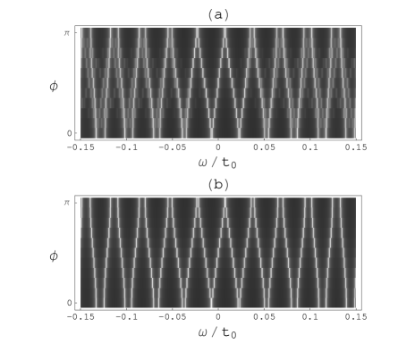
Figure 18: (a) The total density of states of an interacting ring system within the second-order perturbation theory. (b) Total density of states corresponding to the quasiparticle Hamiltonian. The system is described in Fig. 5.

Appendix B Variational ground-state energy

In order to calculate the conductance for interacting systems, we first need to devise a robust method that would allow us to efficiently calculate the ground-state energy of such systems. Note that we need a method that would provide us with the energy of a system with a very large number of sites in the ring. However, the number should still be finite - i.e. we must not perform the calculations in the thermodynamic limit. We made use of the projection method of Gunnarson and Schönhammer Schonhammer75 ; Schonhammer76 ; Gunnarson85 , introduced originally to calculate the ground-state energy of the Anderson impurity model, and extended it to treat the more general Hamiltonian (1).

Let us introduce an auxiliary noninteracting Hamiltonian,

$$\tilde{H}=H_{L}+\tilde{V_{L}}+\tilde{H}_{C}^{\left(0\right)}+\tilde{V}_{R}+H_{R},$$ (70)

with arbitrary matrix elements describing the hopping between the leads and the central region, and the central region itself. Note that these are the same matrix elements as the ones being renormalized in the Fermi liquid quasiparticle Hamiltonian (47). Let us also define a Hilbert space spanned by a set of $4^{M}$ basis functions

$$\left|\psi_{\bm{\alpha}}\right\rangle\equiv P_{\bm{\alpha}}\left|\tilde{0}\right\rangle\equiv\prod_{i\in C}P_{\alpha_{i}}^{i}\left|\tilde{0}\right\rangle,$$ (71)

where $M$ is the number of sites in the central region, $\left|\tilde{0}\right\rangle$ is the ground-state of the auxiliary Hamiltonian (70) containing the same number of electrons as there are in the ground state of the original Hamiltonian, and

$$P_{0}^{i} = \left(1-n_{i\uparrow}\right)\left(1-n_{i\downarrow}\right),$$ (72)

$$P_{\sigma}^{i} = n_{i\sigma}\left(1-n_{i\bar{\sigma}}\right),$$ (73)

$$P_{2}^{i} = n_{i\uparrow}n_{i\downarrow}$$ (74)

are projection operators on unoccupied, singly occupied and doubly occupied site $i$. The original Hamiltonian is diagonalized in the reduced basis set introduced above,

$$H_{\bm{\beta}\bm{\alpha}}=ES_{\bm{\beta}\bm{\alpha}},$$ (75)

with $H_{\bm{\beta}\bm{\alpha}}=\left\langle\psi_{\bm{\beta}}\left|H\right|\psi_{\bm{\alpha}}\right\rangle$ being the matrix elements of the Hamiltonian and $S_{\bm{\beta}\bm{\alpha}}=\left\langle\psi_{\bm{\beta}}\mid\psi_{\bm{\alpha}}\right\rangle$ take into account the fact that the basis functions do not form an orthonormal basis set. The eigenstate with the lowest energy $E_{\tilde{H}}$ of this eigenvalue problem is an approximation to the ground-state energy of the original Hamiltonian. Varying the parameters of the auxiliary Hamiltonian, one can find their optimal values which minimize $E_{\tilde{H}}$. The solution of this minimization problem is the final approximation to the ground-state energy.

Let us consider some simple limits of the problem. In the noninteracting case where $U=0$, one can choose the auxiliary Hamiltonian to be equal to the true Hamiltonian $\tilde{H}=H$. Then the wavefunction $\left|\psi\right\rangle=\sum_{\bm{\alpha}}P_{\bm{\alpha}}\left|\tilde{0}\right\rangle=\left|\tilde{0}\right\rangle=\left|0\right\rangle$ is the exact ground-state wavefunction of the system. Note that applying the same wavefunction ansatz to the interacting case and allowing the matrix elements of the auxiliary Hamiltonian to be renormalized, provides us with the Hartree-Fock solution of the problem. Therefore, the variational method introduced above always gives the ground-state energy which is lower or equal to the corresponding Hartree-Fock ground-state energy. In the limit of the central region being decoupled from the ring, i.e. $V_{L}=V_{R}=0$, the variational method also yields the exact ground-state energy. To prove this statement, let us select the matrix elements of $\tilde{H}$ in such a way that in its ground state there are $m$ electrons in the central region. Then the basis set (71) spans the full Hilbert space for $m$ electrons in the central region. As there is no coupling to the states in the ring, solving the eigenvalue problem (75) provides us with the exact ground state of the problem with a constraint of a fixed number of electrons in the central region. By varying $\tilde{H}$, all the possible values of $m$ can be tested and the one yielding the lowest ground-state energy corresponds to the correct ground state of the system.

The variational wavefunction ansatz can be improved by extending the Hilbert space with additional basis functions, the most promising candidates being of typeGunnarson85

$$\left|\psi_{\bm{\beta}\lambda ji\sigma\bm{\alpha}}\right\rangle=P_{\bm{\beta}}\hat{V}_{\lambda ji\sigma}P_{\bm{\alpha}}\left|\tilde{0}\right\rangle,$$ (76)

where $\hat{V}_{\lambda ji\sigma}=V_{\lambda ji}c_{j\sigma}^{\dagger}d_{i\sigma}+\mathrm{h}.\mathrm{c}.$ and $\lambda$ is a lead index, i.e. either $L$ or $R$. On the other hand, as the size of the Hilbert space increases exponentially with the number of sites in the central region, it might be convenient to limit the basis set to the states obtained by projecting to the central region’s many body states between which fluctuations are possible.

Finally, we state some technical details concerning the evaluation of $H_{\bm{\beta}\bm{\alpha}}$ and $S_{\bm{\beta}\bm{\alpha}}$. It is convenient to express these matrix elements only in terms of quantities related to the central region and the neighboring sites in the leads. As

$$S_{\bm{\beta}\bm{\alpha}}=\left\langle\tilde{0}\left|P_{\bm{\beta}}P_{\bm{\alpha}}\right|\tilde{0}\right\rangle=\left\langle\tilde{0}\left|P_{\bm{\alpha}}\right|\tilde{0}\right\rangle\delta_{\bm{\beta}\bm{\alpha}},$$ (77)

the scalar products between the basis functions are evidently expressed with the central region quantities. The matrix elements of the Hamiltonian can be expressed as

$$H_{\bm{\beta}\alpha} = \left\langle\tilde{0}\left|P_{\bm{\beta}}HP_{\bm{\alpha}}\right|\tilde{0}\right\rangle=$$ (78)

$$= \left\langle\tilde{0}\left|\tilde{H}P_{\bm{\beta}}P_{\bm{\alpha}}\right|\tilde{0}\right\rangle+\left\langle\tilde{0}\left|P_{\bm{\beta}}HP_{\bm{\alpha}}\right|\tilde{0}\right\rangle-$$

$$-\left\langle\tilde{0}\left|\tilde{H}P_{\bm{\beta}}P_{\bm{\alpha}}\right|\tilde{0}\right\rangle=$$

$$= \tilde{E}S_{\bm{\beta}\bm{\alpha}}+\left\langle\tilde{0}\left|P_{\bm{\beta}}\left(V_{L}+H_{\mathrm{C}}+V_{R}\right)P_{\bm{\alpha}}\right|\tilde{0}\right\rangle-$$

$$-\left\langle\tilde{0}\left|\left(\tilde{V}_{L}+\tilde{H}_{\mathrm{C}}^{\left(0\right)}+\tilde{V}_{R}\right)P_{\bm{\alpha}}\right|\tilde{0}\right\rangle\delta_{\bm{\beta}\bm{\alpha}},\quad\quad$$

where $\tilde{E}$ is the ground-state energy of the auxiliary Hamiltonian $\tilde{H}$. In the second and the third term we made use of the fact that lead Hamiltonians $H_{\mathrm{L}}$ and $H_{R}$ commute with the central region projectors and therefore, they cancel out. Again, we succeeded in expressing the matrix elements in terms of central region quantities together with quantities related to the neighboring sites in the leads. Similar results are obtained if the extended basis set of Eq. (76) is used. The matrix elements in Eqs. (77) and (78) need to be calculated in a noninteracting state. Therefore, we can make use of the Wick’s theorem to decompose the expressions into two-operator averages of type $\left\langle\tilde{0}\left|d_{j\sigma}^{\dagger}d_{i\sigma}\right|\tilde{0}\right\rangle$. As a huge number of terms is generated in this procedure, the decomposition was performed automatically by symbolic manipulation of operators. The ground-state energy of the auxiliary Hamiltonian and the two-operator averages can be expressed in terms of the single-electron energies $\tilde{\varepsilon}_{k}$ and wavefunctions $\left|\tilde{\varphi}^{k}\right\rangle$ of $\tilde{H}$ as

$$\tilde{E} = 2\sum_{k\,\mathrm{occ}.}\tilde{\varepsilon}_{k},$$ (79)

$$\left\langle\tilde{0}\left|d_{j\sigma}^{\dagger}d_{i\sigma}\right|\tilde{0}\right\rangle = \sum_{k\,\mathrm{occ}.}\tilde{\varphi}_{j}^{k\ast}\tilde{\varphi}_{i}^{k}.$$ (80)

The sums run only over the single-electron states occupied in the ground state $\left|\tilde{0}\right\rangle$. The eigenvalues $\tilde{\varepsilon}_{k}$ were calculated in a basis in which the Hamiltonian matrix is banded, i.e. linear combinations of local basis functions corresponding to the left lead and right lead sites were introduced to “move” the hopping matrix elements in corners of the matrix close to the diagonal. For each eigenvalue, only the components of the eigenvector related to the central region and neighboring sites were calculated, again taking the special structure of the matrix into account. The procedure used scales with the number of sites in the ring as $\mathcal{O}\left(N^{2}\right)$, which allows one to treat systems with up to 10000 sites in the ring.

References

- (1) J. von Delft and D. C. Ralph, Phys. Rep. 345, 61 (2001).
- (2) L. P. Kouwenhoven et al., in Mesoscopic Electron Transport, edited by L. L. Sohn, L. P. Kouwenhoven, and G. Schön (Kluwer Academic, New York, 1997).
- (3) N. Agraït, A. L. Yeyati, and J. M. van Ruitenbeek, cond-mat/0208239 (unpublished).
- (4) R. H. M. Smit et al., Nature 419, 906 (2002).
- (5) R. Landauer, IBM J. Res. Dev. 1, 233 (1957).
- (6) R. Landauer, Philos. Mag. 21, 863 (1970).
- (7) M. Büttiker, Phys. Rev. Lett. 57, 1761 (1986).
- (8) A. Oguri, Phys. Rev. B 56, 13422 (1997).
- (9) A. Oguri, J. Phys. Soc. Jpn. 70, 2666 (2001).
- (10) Y. Meir and N. S. Wingreen, Phys. Rev. Lett. 68, 2512 (1992).
- (11) A.-P. Jauho, N. S. Wingreen, and Y. Meir, Phys. Rev. B 50, 5528 (1994).
- (12) J. Favand and F. Milla, Eur. Phys. J. B 2, 293 (1998).
- (13) R. A. Molina et al., cond-mat/0209552 (unpublished).
- (14) O. P. Sushkov, Phys. Rev. B 64, 155319 (2001).
- (15) H.-F. Cheung, Y. Gefen, E. K. Riedel, and W.-H. Shih, Phys. Rev. B 37, 6050 (1988).
- (16) A. O. Gogolin and N. V. Prokof’ev, Phys. Rev. B 50, 4921 (1994).
- (17) A. A. Aligia, PRB 66, 165303 (2002).
- (18) P. Prelovšek and X. Zotos, in Lectures on the Physics of Highly Correlated Electron Systems VI, edited by F. Mancini (American Institute of Physics, New York, 2002).
- (19) P. W. Anderson, Phys. Rev. 124, 41 (1961).
- (20) R. E. Peierls, Z. Phys. B 80, 763 (1933).
- (21) S. Datta, Electronic Transport in Mesoscopic Systems (Cambridge University Press, Cambridge, 1995).
- (22) F. Bloch, Phys. Rev. 137, A787 (1965).
- (23) M. Büttiker, Y. Imry, and R. Landauer, Phys. Lett. 96A, 365 (1983).
- (24) V. Meden and U. Schollwoeck, cond-mat/0210515 (unpublished).
- (25) W. Kohn, Phys. Rev. 133, A171 (1964).
- (26) R. A. Jalabert, A. D. Stone, and Y. Alhassid, PRL 68, 3468 (1992).
- (27) J. A. Verges, E. Cuevas, M. Ortuño, and E. Louis, PRB 58, R10143 (1998).
- (28) P. Nozières, Theory of interacting Fermi systems (W. A. Bejnamin, Inc., New York, 1964).
- (29) L. D. Landau, Pis’ma Zh. Eksp. Teor. Fiz. 3, 920 (1956).
- (30) L. D. Landau, Pis’ma Zh. Eksp. Teor. Fiz. 5, 101 (1957).
- (31) P. Nozières, J. Low Temp. Phys. 17, 31 (1974).
- (32) H. Bruus and K. Flensberg, Introduction to many-body quantum theory in condensed matter physics (Oersted Laboratory, Niels Bohr Institute, Copenhagen, 2002).
- (33) D. S. Fisher and P. A. Lee, Phys. Rev. B 23, 6851 (1981).
- (34) A. C. Hewson, The Kondo Problem to Heavy Fermions (Cambridge University Press, Cambridge, 1993).
- (35) K. Yamada and K. Yosida, Prog. Theor. Phys. 76, 621 (1986).
- (36) A. Oguri, J. Phys. Soc. Jpn. 66, 1427 (1997).
- (37) B. Horvatić and V. Zlatić, Phys. Status Solidi B 99, 251 (1980).
- (38) B. Horvatić and V. Zlatić, Solid State Commun. 54, 957 (1985).
- (39) B. Horvatić, D. Šokčević, and V. Zlatić, Phys. Rev. B 36, 675 (1987).
- (40) L. I. Glazman and M. E. Raikh, Pis’ma Zh. Eksp. Teor. Fiz. 47, 378 (1988).
- (41) T. K. Ng and P. A. Lee, Phys. Rev. Lett. 61, 1768 (1988).
- (42) D. Goldhaber-Gordon et al., Nature 391, 156 (1988).
- (43) W. G. van der Wiel et al., Science 289, 2105 (2000).
- (44) P. B. Wiegman and A. M. Tsvelick, Pis’ma Zh. Eksp. Teor. Fiz. 35, 100 (1982).
- (45) P. B. Wiegman and A. M. Tsvelick, J. Phys. C 16, 2281 (1983).
- (46) D. C. Langreth, Phys. Rev. 150, 516 (1966).
- (47) T. Rejec and A. Ramšak, cond-mat/0303258 (to be published in Phys. Rev. B).
- (48) R. A. Molina and R. A. Jalabert, private communication.
- (49) B. L. Altshuler, Y. Gefen, A. Kamenev, and L. S. Levitov, Phys. Rev. Lett. 78, 2803 (1997).
- (50) K. Schönhammer, Z. Phys. B 21, 389 (1975).
- (51) K. Schönhammer, Phys. Rev. B 13, 4336 (1976).
- (52) O. Gunnarson and K. Schönhammer, Phys. Rev. B 31, 4815 (1985).