Bound states of L-shaped or T-shaped quantum wires in inhomogeneous magnetic fields

Abstract

The bound state energies of L-shaped or T-shaped quantum wires in inhomogeous magnetic fields are found to depend strongly on the asymmetric parameter $\alpha=W_{2}/W_{1}$, i.e. the ratio of the arm widths. Two effects of magnetic field on bound state energies of the electron are obtained. One is the depletion effect which purges the electron out of the OQD system. The other is to create an effective potential due to quantized Landau levels of the magnetic field. The bound state energies of the electron in L-shaped or T-shaped quantum wires are found to depend quadratically (linearly) on the magnetic field in the weak (strong) field region and are independent of the direction of the magnetic field. A simple model is proposed to explain the behavior of the magnetic dependence of the bound state energy both in weak and strong magnetic field regions.

I Introduction

Recently, quasi-1D structures, such as quantum wires attract much attention due to the enhanced confinement of the reduced dimension and the possibility of tailoring the electronic and optical properties in applicationsWalck97 –Grundmann98 . Among the structures considered, the opened quantum dot (OQD) is one of the simpler mesoscopic systems in which the essential physics can be studied in great details. An OQD can be formed by additional lateral confinementsLiang97 ; Liang98 or by applying certain magnetic fieldsSolimany95 ; Sim98 . Electrons and holes are trapped at the L-shaped or T-shaped intersections because the single-particle confinement energy can be found to be lower in the intersection of the arms. These OQDs are quite different from the traditional quantum dots, since there remain openings in such OQDs. Electrons in OQD systems are classically unbounded. However, recent experimental photoluminescence spectroscopy analysesWalck97 ; Glutsch97 ; Langbein96 have manifested that there are bound states in such OQDs. The existence of bound states in OQDs essentially shows the confinement effect of the mesoscopic geometry in quantum mechanical region.

The exploration of the properties of bound states is a key to understand some recent optical and electrical experiments on T-shaped quantum wires and quantum dotsGlutsch97 ; Langbein96 ; Brinkmann97 ; Grundmann98 ; Liang97 ; Liang98 . The magneto-photoluminescence of T-shaped wires were measured recentlySomeya95 . The energy shift $\Delta E$ of PL peaks with magnetic field $B$ applied perpendicular to the wire axis and parallel to the stem wire was measured. In these experiments, the information of exciton binding energy can be provided from the photoluminescence spectroscopy. However, it is unable to identify exactly the exciton binding energies unless we have the knowledge of the confinement energy of either an electron or a hole in quantum wires or quantum dots. Because they can not be extracted directly from magneto-optical data due to the nonlinearity of the systems. In a theoretical calculation of magneto-excitons in T-shaped wiresBryant01 , the observed field dependence of the exciton states for weak confinement was reproduced, however, the diamagnetic shifts calculated from perturbation theory is fail to describe the experimental results.

In this work, we consider two-dimensional OQDs which are formed at the intersection of the arms of L-shaped or T-shaped quantum wires when additional magnetic fields are applied perpendicular to the plane of arms. A T-shaped quantum wire can be obtained by first growing a $GaAs/Al_{x}Ga_{1-x}As$ superlattice on a (001) substrate, after cleavage, a $GaAs$ quantum wire is grown over the exposed (110) surface, resulting in a T-shaped region where the electron or hole can be confined on a scale of 5-10 nm. The bound state energy of a charged particle (e.g. electron) in such an opened quantum dot will be affected by the asymmetric geometry of the system and the applied inhomogeneous magnetic fields. Intuitively, when the confinment along one arm of the quantum wire is increased, confinment along the orthogonal arm will decrease, because squeezing the electron or hole in one arm will result in pushing the electron or hole out of the quantum wire through the other arm. These pheonomena are not only interesting in physics but also have no classical correspondence. To our knowledge this squeezing effect have not been studied thoroughly. Furthermore, T-shaped semiconductor quantum wires could be exploted as three-terminal quantum interference devices, thus the study on the L-shaped or T-shaped quantum wire is also important in practical applications.

II Formulation

In the present work, a two-dimensional T-shaped (TOQW) or L-shaped opened quantum wire (LOQW) is considered. A quantum dot with an area of $W_{1}\times W_{2}$ is formed in the intersection region while magnetic fields $B_{1}$, $B_{2}$ and $B_{3}$ are applied perpendicularly to the other subregions of the TOQW as shown in Fig. 1(a). The LOQW as shown in Fig. 1(b) can be regarded as a transformation of TOQW in which the arm 2 is cut off.

Figure 1: The illustrations of the geometries of OQDs in (a) TOQW and (b) LOQW systems.

For simplicity, the boundaries are assumed to be a hard–wall confinement potential, leading to the formation of a magnetically confined cavity in which the confinement of electron is enhanced. The transverse potential inside the TOQW or LOQW is assumed to be zero. The magnetic fields are assumed to be uniform in each individual subregion. Landau gauge is chosen for the vector potential in different subregions:

$$\mathbf{{A}(x,y)} \mathbf{=}$$

$$\mathbf{\left\{\begin{array}[]{ll}\begin{array}[]{l}(0,B_{1}(x+0.5W_{2}))=(-B_{1}y,0)\\ +\nabla B_{1}(x+0.5W_{2})y,\end{array}&\mbox{in region I;}\\ \begin{array}[]{l}(0,B_{2}(x-0.5W_{2})=(-B_{2}y,0)\\ +\nabla B_{2}(x-0.5W_{2})y,\end{array}&\mbox{in region II;}\\ \begin{array}[]{l}(-B_{3}(y-0.5W_{1}),0)=(0,B_{3}x)\\ -\nabla B_{3}x(y-0.5W_{1}),\end{array}&\mbox{in region III};\\ (0,0),&\mbox{in region IV.}\end{array}\right.}$$

The form of gauge guarantees the continuity of the vector potential at each interface. The origin is chosen at the center of the intersection region.The wavefunctions of the bound state $n$ of an electron for different subregions $I,II,III.IV$ are

$$\begin{array}[]{ll}\begin{array}[]{l}\Psi_{n}^{I}=e^{-i(x+0.5W_{2})yeB_{1}/\hbar}\\ \times\left[\sum_{m}r_{mn}e^{ik_{m}^{I}(x+0.5W_{2})}\Phi_{m}^{I}(y)\right]\end{array}&\mbox{in region I;}\\ \begin{array}[]{l}\Psi_{n}^{II}=e^{-i(x-0.5W_{2})yeB_{2}/\hbar}\\ \times\left[\sum_{m}t_{m}e^{ik_{mn}^{I}(x-0.5W_{2})}\Phi_{m}^{II}(y)\right]\end{array}&\mbox{in region II;}\\ \begin{array}[]{l}\Psi_{n}^{III}=e^{ix(y-0.5W_{1})eB_{3}/\hbar}\\ \times\left[\sum_{m}s_{mn}e^{ik_{m}^{II}(y-0.5W_{1})}\Phi_{m}^{III}(x)\right]\end{array}&\mbox{in region III;}\end{array}$$

$$\Psi_{n}^{IV} = \sum_{j}f_{j}(y)\left[a_{jn}\sin k_{j}^{\prime}(x-0.5W_{2})+b_{jn}\sin k_{j}^{\prime}(x+0.5W_{2})\right]$$ (5)

$$+c_{jn}g_{j}(x)\sin k_{j}^{{}^{\prime\prime}}(y+0.5W2)$$

where

$$f_{j}(y) = \sqrt{\frac{2}{W_{1}}}\sin(\frac{j\pi}{W_{1}}y),-0.5W_{1}\leq y\leq 0.5W_{1}$$ (6)

$$g_{j}(x) = \sqrt{\frac{2}{W_{2}}}\sin(\frac{j\pi}{W_{2}}x).-0.5W_{2}\leq x\leq 0.5W_{2}$$ (7)

$k_{j}^{\prime}=[k^{2}-(j\pi/W_{1})]^{1/2}\,$,$\,k_{j}^{{}^{\prime\prime}}=[k^{2}-(j\pi/W_{2})]^{1/2}$ and $k_{m}^{i},\,i=I,II,III,\cdots$. Now drop the subscript $n$ and substitute Eqs.(2) into the Schrödinger equation. After solving it numerically, one obtains eigen-wave-numbers $\{k_{m}^{I}\}$, $\{k_{m}^{II}\}$, $\{k_{m}^{III}\}$, the expansion coefficients in Eqs. (II) and (5), and the eigen-wave-functions $\{\Phi_{m}^{I}(y)\}$, $\{\Phi_{m}^{II}(x)\}$, $\{\Phi_{m}^{III}(x)\}$.

III Results and Discussions

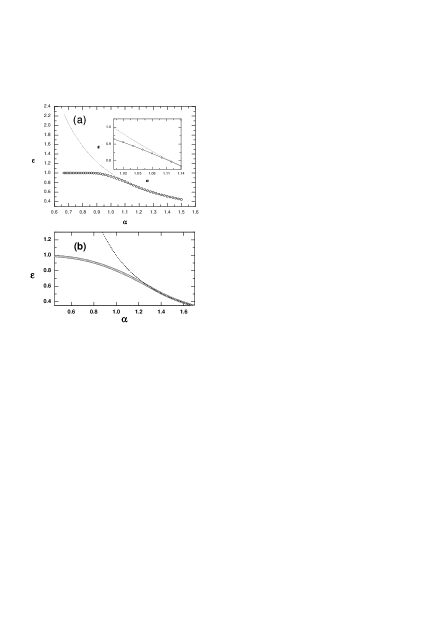
Figure 2: (a).The bound state energy $\varepsilon$ versus the asymmetric ratio $\alpha=W_{2}/W_{1}$ at zero magnetic field strength. Open circle is our result. The dotted line is the curve $1/\alpha$ as a guide to eyes. $E_{1}=\frac{\hbar^{2}\pi^{2}}{2m^{\ast}W_{1}^{2}}$ is the first threshold energy of arm 1 (the region I). (b).The bound state energy $\varepsilon$ of a TOQW plotted in unit of $E_{1}$ as a function of $\alpha$. The bound state energy of the electron approaches to unity for $\alpha<<1$ and can be approximately expressed by the curve $1/\alpha^{2}$ for $\alpha\geq 1.33.$

Fig. 2(a) presents the calculated bound state energy of an electron in a LOQW as a function of arm ratio $\alpha$. The bound state energy of the electron is expressed in terms of the dimensionless quantity $\varepsilon=E/E_{1}$, where $E_{1}=\frac{\hbar^{2}\pi^{2}}{2m^{\ast}W_{1}^{2}}$ is the first subband energy in arm 1. One can note from the figure that the bound state energy becomes smaller as the arm ratio $\alpha$ becomes larger. For $\alpha=1$ (i.e. $W_{1}=W_{2}$), $r_{m}=t_{m}$ at zero magnetic field, the bound state energy is $0.92964E_{1}$. The bound state energy $\varepsilon$ goes down and behaves like the curve $1/\alpha^{2}$ as the $\alpha$ is increased larger than $1.14$. A deviation from the curve $1/\alpha^{2}$ is observed in the region of $\alpha\leq 1.14$ as shown in the inset of Fig. 2(a). The result can be ascribed to the fact that the bound state energy of the electron matches the subband energy of arm 2 due to the lateral confinement of region II. Since in this circumstance, $1/\alpha^{2}(\pi/W_{1})^{2}$ is equal to $(\pi/W_{2})^{2}$, which is the first subband level of the vertical wire. As the width $W_{2}$ becomes larger and larger, the energy level becomes lower and lower, and gradually coincides with the bound state level of the electron. Thus electron is unable to be bounded in the corner region any more. As the asymmetry becomes more prominently, the electronic energy becomes larger than the bottom of the subband of the wider arm. However, if the energy of the electron state is less than or just equal to the subband bottom, the electron is still bounded inside the corner and does not move to the right or to the left.

Figure 3: The bound state energy $\varepsilon$ versus the field strength $f$. (a) for both arms being acted by the magnetic fields in LOQW system. (b) for only one arm being acted by the magnetic fields. The dimensionless field strength $f$ is normalized by $E_{1}$.

Fig. 2(b) shows the bound state energy of the electron in a TOQW as a function of $\alpha$. The bound state energy approaches unity as the width of the vertical arm becomes very small, and behaves like the curve $1/\alpha^{2}$ while $\alpha$ becomes larger. This is similar to the case of a LOQW. The reason of this result can be understood intuitively that the wavefunction of the electron is purged out of the vertical arm when it becomes very narrow, therefore, the energy of this state is close to the first threshold energy $E_{1}$ of the horizontal arm with a width of $W_{1}$. This bound state of the electron exists as long as the vertical arm is infinite long, and is expected to disappear owing to the effect of leakage if the arms is finite in length.

The calculated bound state energy of a symmetric LOQW in magnetic fields as a function of the field strength $f=\hbar\omega_{c}/E_{1}$ is shown in Fig. 3(a) and (b), where $\omega_{c}$ is cyclotron frequency of the electron. One can observe that the bound state always exists when the magnetic field is applied to both arms. The bound state depends linearly on the magnetic field in weak field region while quadratically in strong field region. increases monotonically as the magnetic field increases. However, the energy of the bound state is pushed up by the applied magnetic field, and then it goes up to $E_{1}$ when the magnetic field is applied to only one arm. Thus, the electron can escape via the field free arm. Fig. 4 presents the confinement energy in a symmetric TOQW versus the field strength when (a) all arms are acted by the same magnetic field $B$, (b) the two horizontal arms are acted by the same magnetic field, and (c) only the vertical arm is acted by the magnetic field. The same quadratic dependence of magnetic field of the bound state energy is revealed again for weak field, and the linear dependence appears in the strong field region as the case of LOQW. Obviously, the bound state of the electron in a TOQW system locates deeper than that in a LOQW, thus, the TOQW system has a weaker confinement potential than the LOQW system.

The magnetic fields introduce a depleting effect on electrons and add an extra potential surrounding the intersection region. The effective potentials introduced by the magnetic fields are $k$–dependent. For the bound state, these effective potentials are complex due to the pure imaginary {$k$}. One expects intuitively that the magnetic field adds the lowest Landau level $\frac{\hbar\omega_{c}}{2}=\frac{\hbar eB}{2m^{\ast}}$ directly to the quantum dot system an extra potential. Such levels are added into the wire arm regions. However, the field plays another role due to the essential physics of the magnetism. Qualitatively, one can understand the effect induced by the magnetic field on the bound state by considering an one-dimensional shallow quantum well with finite height $U_{0}$. In the limit of shallow well, there is only one bound state exists in the well. Its level energy is given by $E_{0}=U_{0}-(m^{\ast}W^{2}/2\hbar^{2})U_{0}^{2}$, which is near the top of the well. As the magnetic field applies to the system, the bound state energy changes because the potential height is changed to $U_{0}+\frac{1}{2}\hbar\omega_{c}$. The variation of the state level depends linearly on the potential height, i.e.

$$\frac{\partial E_{0}}{\partial U_{0}}=1-\frac{m^{\ast}W^{2}}{\hbar^{2}}U_{0},$$

The variation of the state level by taking account the depletion effect of the magnetic field is assumed as

$$\frac{\partial E_{0}}{\partial W}=-\frac{m^{\ast}W}{\hbar^{2}}U_{0}^{2}.$$

Obviously, once we take the well shrunk into account, the quadratic form of the dependence of magnetic field has to be considered also. This simple model manifests the important geometric effect and the essential properties of magnetism at the same time. Since the shrinking of the geometric scale is no longer prominent in strong magnetic field region, the influence of the magnetic field on the electron becomes smaller. Thus, the bound state energy depends simply on the added effective potential, such that it seems likely to depend linearly on the magnetic field in the strong magnetic field region.

Figure 4: The bound state energy $\varepsilon$ of T-shaped QW as a function of the field strength $f$. Curve (a) for all arms being acted by magnetic fields. The field strength $f$ is normalized by $E_{1}$. Curve (b) for the horizontal arms being acted by magnetic fields, and curve (c) for only vertical arm being acted by magnetic field. The dimensionless field strength $f$ is normalized by $E_{1}$.

IV Summary

The effects of the asymmetric geometry and surrounding inhomogeneous magnetic fields on the bound state of L-shaped or T-shaped quantum wires are studied. When $\alpha$ increases, the bound state energy of the electron is lower as expected. On the other hand, when the applied magnetic field increases, the bound state level of the electron is pushed higher and higher and the electron begins to be unbounded if there is an arm with finite length which offers a passway for electron to leak out. Generally, the bound state level of an electron in a TOQW system is lower than that in LOQW system. This fact reflects the weaker confinement of the geometry. Parabolic dependence of the bound state energy of the electron in weak field region on the field strength is understood as a result of the depletion effect. In the contrast, linear dependence in high field region is found to be resulted from the additional effective potential due to the magnetic field.

This work is supported partially by National Science Council, Taiwan under the grant number NSC90-2112-M-009-018.

References

- (1) S. N. Walck, T. L. Reinecke, and P.A. Knipp, Phys. Rev. B 56, 9235(1997).
- (2) S. Glutsch, F. Bechstedt, W. Wegscheider, and G. Schedekbeck, Phys. Rev. B 56,4108 (1997).
- (3) W. Langbein, H. Gislason, and J. M. Hvam, Phys. Rev. B 54, 14595 (1996).
- (4) T. Someya, H. Akiyama, and H. Sakaki, Phys. Rev. Lett. 74, 3664 (1995); Appl. phys. Lett. 66, 3672 (1995); Phys. Rev. Lett.76, 2965 (1996); H. Akiyama, T. Someya, M. Yoshita, T. Sakai, and H. Sasaki, Phys. Rev. B 57, 3765 (1998).
- (5) A. Yacoby, H. L. Stormer, N. S. Wingreen, L. N. Pfeiffre, K. W. Baldwin, and K. W.West, Phys. Rev. Lett. 77, 4612(1996).
- (6) R. Šordan and K. Nikolić, Appl. Phys. Lett. 68, 3599 (1996); 71, 803 (1997).
- (7) G. Golodoni, F. Rossi, E. Molinari, and A. Fasolino, Phys. Rev. B 55, 7110 (1997); F. Rossi, G. Goldoni, and E. Molinari, Phys. Rev. Lett. 78, 3527 (1997).
- (8) D. Brinkmann and G. Fishman, Phys. Rev. B 56, 15211 (1997).
- (9) M. Grundmann, O. Stier, and D. Bimberg, Phys. Rev. B 58, 10557 (1998).
- (10) C.-T. Liang, I. M. Castleton, J. E. F. Frost, C.H.W. Barnes, C. G. Smith, C. J. B. Ford, D. A. Ritchie, and M. Pepper, Phys. Rev. B 55, 6723 (1997).
- (11) C.-T. Liang, M. Y. Simmons, C. G. Smith, G. H. Kim, D. A. Ritchie, and M. Pepper, Phys. Rev. Lett. 81, 3507 (1998).
- (12) L. Solimany and B. Kramer, Solid state Comm. 96, 471 (1995).
- (13) H.-S. Sim, K.-H, Ahn, K.-J. Chang, G. Ihm, N. Kim, and S.-J. Lee, Phys. Rev. Lett. 80, 1501 (1998).
- (14) G.W. Bryant and Y.B. Band, Phys. Rev. B 63, 115304 (2001).