Probing Polyelectrolyte Elasticity Using Radial Distribution Function

Abstract

We study the effect of electrostatic interactions on the distribution function of the end-to-end distance of a single polyelectrolyte chain in the rodlike limit. The extent to which the radial distribution function of a polyelectrolyte is reproduced by that of a wormlike chain with an adjusted persistence length is investigated. Strong evidence is found for a universal scaling formula connecting the effective persistence length of a polyelectrolyte with its linear charge density and the Debye screening of its self-interaction. An alternative definition of the electrostatic persistence length is proposed based on matching of the maximum of the distribution with that of an effective wormlike chain, as opposed to the traditional matching of the first or the second moments of the distributions. It is shown that this definition provides a more accurate probe of the affinity of the distribution to that of the wormlike chains, as compared to the traditional definition. It is also found that the length of a polyelectrolyte segment can act as a crucial parameter in determining its elastic properties.

I Introduction and Summary

The close connection between the elasticity of rodlike cytoskeletal polymers and the mechanical properties of cells has been extensively documented Alberts (2002); Eichinger et al. (1996); Janmey (1999). For example, actin filaments are known to play a crucial role in the recovery of eukaryotic cell shape in the face of the stresses imposed by cell movement, growth and division. Furthermore, the stiffness of DNA constrains and controls both its storage in the cell nucleus and access to it by the proteins and enzymes that are central to its role in biological processes. However, there is, as yet, no complete, quantitative understanding of the relationship between the elastic attributes of these polymers and the influences that control them. Such an understanding is crucial to the development of a general description of the functionality of polymers.

An additional spur to an increased focus on the connection between first-principle energetics and the elastic characteristics of polyelectrolytes is the fact that experimental techniques have been developed that allow for the imaging of single filaments in solution Helfer et al. (2000). This means that it is now possible to test models and theoretical predictions at the level of a single chain polymer.

The key challenge in this area is to produce a theoretical analysis that connects the electrostatic interactions and local energetics of a polyelectrolyte with its overall mechanical properties. In the case of neutral chain polymers, the wormlike chain (WLC) model of Kratky and Porod Kratky and Porod (1949) provides a powerful and convenient characterization of flexibility, through the persistence length, which is the decay length of the tangent-tangent correlation function of a stiff, inextensible polymer chain. The lack of a similarly inclusive and readily implemented model for polyelectrolytes has been addressed through the application of the WLC model to polyelectrolytes, with the introduction of an effective, “electrostatic,” persistence length Odijk (1977); Skolnick and Fixman (1977). The shortcomings of this notion, which replaces the many length scales in a polyelectroyte by a single effective persistence length, have been commented on Odijk (1977); Barrat and Joanny (1993); Ha and Thirumalai (1999). Additionally, codifying electrostatic interactions in terms of single length ignores the possibility of chain collapse resulting from fluctuation-induced self-attraction Golestanian et al. (1999).

If a suitably modified WLC model did, indeed, provide a working model for the calculation of the conformational properties of polyelectrlytes, then a number of powerful results could be brought to bear on the study of this system. Among the more useful of these is the recently derived end-to-end distribution Gennes (1979) of short segments of an inextensible polymer Wilhelm and Frey (1996). The distribution, which is expected to apply to segments whose backbone length is less than the persistence length of the polymer—the rodlike limit—was shown to be accurate both in that limit and somewhat outside it. The distribution possesses the virtue that it can, in principle, be utilized in the analysis of currently feasible experiments on polymers in the rod-like limit Le Goff . One can, then, determine whether or not the WLC model accurately reflects the properties of the polymer segments in question. If the model has been shown to apply, then the fit of the distribution to the data directly yields the persistence length and, hence, the elastic modulus of the polymer.

An additional advantage of the end-to-end distribution function is that it is a function, rather than a number. That is, the end-to-end distribution function contains, at least in principle, an infinitely greater amount of information than can be encoded in a single quantity. The distribution thus represents a more comprehensive characterization of the elastic and thermal characteristics of a charged semiflexible chain. In this sense, it provides one with an opportunity to disentangle the actions of electrostatic and mechanical interactions as they affect the conformational properties of a fluctuating polyelectrolyte.

In this article, we calculate the end-to-end distribution of a charged, inextensible, semiflexible chain. This distribution is then utilized to address two central questions relating to the conformational statistics of a polyelectrolyte. Those questions are:

1. Under what circumstances is the end-to-end distribution of the PE reproduced by the end-to-end distribution of a WLC with an adjusted persistence length?

2. Under what circumstances will the effective persistence length of a PE be as predicted by existing formulas?

As will be shown below, we are able to identify regimes associated with strong electrostatic coupling, weak screening, or high intrinsic flexibility of the PE, in which the end-to-end distribution deviates from that of a WLC. We are also able to identify the regions in which this approximation is accurate. The concept of electrostatic persistence length is examined, and an alternative definition of this important length scale is suggested. Our newly-defined electrostatic persistence length is compared with a well-known and widely-utilized formula for the persistence length of a stiff, charged rod Odijk (1977). The new electrostatic persistence length is found to obey a universal crossover scaling law.

The rest of the paper is organized as follows: Section II describes the model that we use to study the elasticity of stiff PE’s. This model is a straighforward extension of the Kratky-Porod model of a WLC. The energy of this system consists of the mechanical energy required to induce a local curvature in the chain and the screened electrostatic repulsion between the charges on the chain, which are assumed to be uniformly distributed along it, in the form of a constant linear charge density. The distribution function of the end-to-end distance of this chain is then introduced and given a precise mathematical form. An expression for this distribution is derived, under the assumption that the chain does not undergo too much of a distortion from it minimum-energy configuration as a straight line. That expression, which is based on the eigenvalues of the Hamiltonian of the PE forms the basis of all the results reported in this article. Details of the expansion of the electrostatic self-interaction about the rodlike configuration are presented in Appendix A. Section III is devoted to a discussion on the structure of those energy eigenvalues. The influence of the electrostatic interaction, which is most pronounced at on the lower eigenvalues, is discussed. Also discussed are the methods and criteria utilized to guarantee the numerical reliability of the end-to-end distribution. Section III.2 briefly summarizes exact results that have been obtained for the eigenvalues of the Hamiltonian consisting entirely of the unscreened Coulomb interaction. These results are relevant to the conformational statistics of a chain stiffened entirely by such interactions. A more detailed description of the way in which the results were obtained is relegated to Appendix B. Section IV presents the results for the distribution function in various situations. Particular attention is paid to the question of the relationship between the distribution function calculated here and the corresponding end-to-end distribution function of a neutral rod-like semiflexible polymer. Section V scrutinizes the concept of electrostatic persistence length. The point of comparison is a general formula for the persistence length, introduced by Odijk. We discuss the ways in which a persistence length can be extracted from the end-to-end distribution, and we justify the method of choice in this investigation, which is based on the location of the maximum of the end-to-end distribution. We find that our results are consistent with Odijk’s formula when the distribution we calculate can be made to collapse on the end-to-end distribution of an uncharged WLC. Conversely, our results do not agree with the Odijk formula when the distribution is inconsistent with that of a WLC with adjusted persistence length. We find that the effective persistence length of the end-to-end distribution function can be described by a “universal” formula, incorporating a scaling form and a new, unexpected power law. This formula holds whether or not the effective persistence length is described by Odijk’s expression. Section VI focuses on this behavior of the effective persistence length. Section VII discusses issues related to the moments of the distribution, and the use of those moments to define a persistence length. Section VIII concludes the paper.

II Model Elasticity for Polyelectrolytes

Because of the inextensibility of the polyelectrolytes under consideration Wilhelm and Frey (1996); Odijk (1995), we adopt Kratky and Porod wormlike chain model Kratky and Porod (1949) to describe the bending energy of the chain. In this model, polymers are represented by a space curve ${\bf r}(s)$ as a function of the arc length parameter $s$. The total energy of the chain, which is the sum of the intrinsic elasticity and the electrostatic energy can be written as

$$\frac{\cal H}{k_{\rm B}T}=\frac{\ell_{p0}}{2}\int_{0}^{L}ds\left(\frac{d{\bf t}(s)}{ds}\right)^{2}+\frac{\beta}{2}\int_{0}^{L}dsds^{\prime}\frac{e^{-\kappa|{\bf r}(s)-{\bf r}(s^{\prime})|}}{|{\bf r}(s)-{\bf r}(s^{\prime})|},$$ (1)

where ${\bf t}$ is the unit tangent vector. We do not take into account the fluctuations in the charges localized to the chain and in the counterion system that can give rise to attractive interactions leading to chain collapse Golestanian et al. (1999). The above equation contains several different length scales: (1) the average separation between neighboring charges $b$, (2) the Debye screening length $\kappa^{-1}$, (3) the Bjerrum length $\ell_{\rm B}=e^{2}/\epsilon k_{\rm B}T$, the quantity $\epsilon$ being the dielectric constant of the ion-free solvent, (4) the intrinsic persistence length $\ell_{p0}$, and (5) the total chain length, $L$. Two of these length scales, namely $\ell_{\rm B}$ and $b$, always appear together in the form of the ratio $\ell_{\rm B}/b^{2}$, which is denoted by $\beta$ in Eq. (1).

We can thus construct three independent dimensionless ratios: $\beta L$ (a measure of the strength of the electrostatic interactions), $\kappa L$ (a measure of the degree of screening), and $\ell_{p0}/L$ (a measure of the intrinsic flexibility). A comprehensive exploration of parameter space entails the examination of the effects associated with a change in the electrostatic coupling and the degree of screening. We focus on inextensible chains that are substantially stiffened by their bending energy ($\ell_{p0}\sim L$) and for which the bending energy alone is insufficient to keep the chain nearly rod-like ($\ell_{p0}\ll L$). The chain is assumed to be sufficiently stiff that excluded volume does not play a role.

The end-to-end distribution function is defined as follows:

$${\cal G}({\bf r})=\langle\delta({\bf r}-{\bf R})\rangle,$$ (2)

where ${\bf R}={\bf r}(L)-{\bf r}(0)$. The average in Eq. (2) is over an ensemble of PE chains. The function ${\cal G}({\bf r})$ is, then, the probability that a given chain in the ensemble will have an end-to-end distance equal to ${\bf r}$. We make use of the procedure that Wilhelm and Frey have implemented to calculate the end-to-end distribution function for inextensible neutral polymers Wilhelm and Frey (1996). In order to calculate ${\cal G}({\bf r})$ in the vicinity of the rodlike limit we restrict our consideration to regions in which the combination of intrinsic stiffness and repulsive strength of the Coulomb interaction keeps the chains in their rodlike limit not . Using the integral representation of the $\delta$ function, we can write ${{\cal G}(r)}$ as

$${\cal G}({\bf r})={1\over{\cal Z}}\int\frac{d^{3}{\bf\mu}}{(2\pi)^{3}}\int{\cal D}{\bf t}(s)$$ (3)

$$\times\exp\left\{i{\bf\mu}\cdot{\bf r}-i{\bf\mu}\cdot\int_{0}^{L}ds\;{\bf t}(s)-\frac{\ell_{p0}}{2}\int_{0}^{L}ds\left(\frac{d{\bf t}(s)}{ds}\right)^{2}\right.$$

$$\left.+\frac{\beta}{2}\int_{0}^{L}dsds^{\prime}\;\frac{e^{-\kappa|{\bf r}(s)-{\bf r}(s^{\prime})|}}{|{\bf r}(s)-{\bf r}(s^{\prime})|}\right\},$$

in which ${\cal Z}=\int{\cal D}{\bf t}(s)\;\exp\left(-{\cal H}/{k_{\rm B}T}\right)$. We then parameterize the unit tangent field as

$${\bf t}(s)={(a_{x}(s),a_{y}(s),1)\over\sqrt{1+a_{x}^{2}(s)+a_{y}^{2}(s)}},$$ (4)

in which the constraint of inextensibility is manifestly satisfied.

Making use of the relation ${\bf r}(s)-{\bf r}(s^{\prime})=\int_{s}^{s^{\prime}}du\;{\bf t}(u)$, we expand the screened Coulomb interaction about the rodlike configuration to quadratic order in ${\bf a}(s)=(a_{x}(s),a_{y}(s))$ (see Appendix A for details). We then use the series expansion ${\bf a}(s)=\sqrt{2}\sum_{n=0}^{\infty}{\bf A}_{n}\cos\left(\frac{n\pi s}{L}\right)$ as appropriate for the open-end boundary condition, and assume for simplicity that ${\bf r}$ is, on average, oriented along the $z$-axis so that ${\bf A}_{0}={1\over\sqrt{2}}\int_{0}^{L}ds\;{\bf a}(s)=0$. Substituting Eq. (20) in Eq. (3), we obtain

$${\cal G}({\bf r})={1\over{\cal Z}}\int\frac{d^{3}{\bf\mu}}{(2\pi)^{3}}\int\prod_{n=1}^{\infty}d^{2}A_{n}$$ (5)

$$\times\exp\left\{i{\bf\mu}\cdot{\bf r}-i\mu_{z}L+\frac{i\mu_{z}L}{2}\sum_{n=1}^{\infty}{\bf A}_{n}^{2}\right.$$

$$\left.-\frac{\ell_{p0}}{2L}\sum_{n=1}^{\infty}(n\pi)^{2}{\bf}A_{n}^{2}-\frac{\beta L}{2}\sum_{n,m=1}^{\infty}{\bf A}_{n}\cdot{\bf A}_{m}E_{nm}\right\},$$

where

$$E_{nm} = {L\over\pi^{2}nm}\int_{-\infty}^{\infty}{dk_{z}\over 2\pi}\left(k_{z}^{2}+\kappa^{2}\right)\ln\left[\frac{(\pi/b)^{2}+\kappa^{2}+k_{z}^{2}}{\kappa^{2}+k_{z}^{2}}\right]$$ (6)

$$\times \left\{\cos\left[{\pi\over 2}(n-m)\right]\left[\frac{\sin\left({k_{z}L\over 2}\right)\sin\left({k_{z}L\over 2}-{\pi(n-m)\over 2}\right)}{k_{z}\left[k_{z}-{(n-m)\pi/L}\right]}-\frac{\sin\left({k_{z}L\over 2}-{\pi n\over 2}\right)\sin\left({k_{z}L\over 2}-{\pi m\over 2}\right)}{(k_{z}-{n\pi/L})(k_{z}-{m\pi/L})}\right]\right.$$

$$\left.-\cos\left[{\pi\over 2}(n+m)\right]\left[\frac{\sin\left({k_{z}L\over 2}\right)\sin\left({k_{z}L\over 2}-{\pi(n+m)\over 2}\right)}{k_{z}[k_{z}-(n+m)\pi/L]}-\frac{\sin\left({k_{z}L\over 2}+{\pi n\over 2}\right)\sin\left({k_{z}L\over 2}-{\pi m\over 2}\right)}{(k_{z}+n\pi/L)(k_{z}-m\pi/L)}\right]\right\}$$

$$+ {1\over L}\int_{-\infty}^{\infty}{dk_{z}\over 2\pi}\left(k_{z}^{2}+\kappa^{2}\right)\ln\left[\frac{(\pi/b)^{2}+\kappa^{2}+k_{z}^{2}}{\kappa^{2}+k_{z}^{2}}\right]\left\{\frac{d^{2}}{dk_{z}^{2}}\left[\frac{\sin^{2}\left({k_{z}L\over 2}\right)}{k_{z}^{2}}\right]\right\},$$

are the elements of the electrostatic energy matrix in the cosine basis set, with $b$, the average separation between neighboring charges, serving as the short distance cutoff.

Performing the functional integral over ${\bf A}_{n}$, we then obtain

$${\cal G}({\bf r})={1\over L}\delta(r_{x})\delta(r_{y})\int_{-\infty}^{\infty}{d\omega\over 2\pi}\;e^{i\omega(1-r_{z}/L)}\frac{\det\left[{\bf T}\right]}{\det\left[{\bf T}+i\omega{\bf I}\right]},$$ (7)

where ${\bf T}=(n\pi)^{2}(\ell_{p0}/L){\bf I}+\beta L{\bf E}$, ${\bf I}$ is the identity matrix, and $\omega=-{\bf\mu}_{z}L$. Note that the distribution function in Eq. (7) is manifestly normalized to unity, i.e. $\int d^{3}{\bf r}\;{\cal G}({\bf r})=1$. We can then integrate over the orientational degrees of freedom to find the radial distribution function

$$G(r)=r^{2}\int_{0}^{\pi}\sin\theta d\theta\int_{0}^{2\pi}d\phi\;{\cal G}({\bf r}),$$ (8)

that is subject to the normalization $\int_{0}^{\infty}dr\;G(r)=1$. Using ${\bf r}=(r\sin\theta\cos\phi,r\sin\theta\sin\phi,r\cos\theta)$, we obtain

$$G(r)={1\over L}\int_{-\infty}^{\infty}{d\omega\over 2\pi}\;\left[e^{i\omega(1-r/L)}+e^{i\omega(1+r/L)}\right]\frac{\det\left[{\bf T}\right]}{\det\left[{\bf T}+i\omega{\bf I}\right]},$$ (9)

which can be rewritten as

$$G(r) = {1\over L}\int_{-\infty}^{\infty}{d\omega\over 2\pi}\;\left[e^{i\omega(1-r/L)}+e^{i\omega(1+r/L)}\right]$$ (10)

$$\times\prod_{n=1}^{\infty}{\left(\lambda_{n}\over\lambda_{n}+i\omega\right)},$$

in terms of the eigenvalues, $\lambda_{n}$, of the matrix ${\bf T}$. Contour integration then yields

$$G(r)=\sum_{n=1}^{\infty}\lambda_{n}f(n)\left[e^{-\lambda_{n}(1-r/L)}\theta(L-r)+e^{-\lambda_{n}(1+r/L)}\right],$$ (11)

with

$$f(n)=\prod_{i\neq n}\left({\lambda_{i}\over\lambda_{n}-\lambda_{i}}\right).$$ (12)

In the above expressions, the second term in brackets contributes negligibly in the rodlike limit, because even the smallest eigenvalues are considerably larger than unity in this regime. Neglecting this term thus yields

$$G(r)={\cal N}\theta(L-r)\sum_{n=1}^{\infty}\lambda_{n}f(n)\;e^{-\lambda_{n}(1-r/L)},$$ (13)

where the normalization prefactor ${\cal N}$ is used to compensate for the small error caused by neglecting the second contribution. This prefactor can be found by enforcing normalization on $G(r)$.

III Energy Eigenvalues

III.1 General Results

To obtain the radial distribution function we must determine the spectrum of the effective Hamiltonian ${\bf T}$. Since this effective Hamiltonian incorporates the energy cost when the PE deviates from a rodlike configuration, the spectrum of its eigenvalues $\lambda_{n}$ should be positive and a monotonically increasing function of the index $n$. Note that it is the lowest eigenvalues that exert the dominant influence on the radial distribution function.

Figure 1 shows the eigenenergies of the electrostatic interaction ${\bf E}$ at $\kappa L=10$. To emphasize the importance of the finite length $L$ of the PE, we calculate the matrix $E_{nm}$ [using Eq. (6)] in the limit $L\to\infty$, and find

$$E_{nm}(L\to\infty) = {1\over 2}\delta_{nm}\left\{\left[{(n\pi)^{2}+(\kappa L)^{2}\over(n\pi)^{2}}\right]\right.$$ (14)

$$\left.\ln\left[(n\pi)^{2}+(\kappa L)^{2}\over(\kappa L)^{2}\right]-1\right\}.$$

This limit can be achieved in Eq. (14) by using $\lim_{L\to\infty}\sin\left[L\left({k_{z}\over 2}-{n\pi\over 2L}\right)\right]/\left({k_{z}\over 2}-{n\pi\over 2L}\right)=2\pi\delta(k_{z}-n\pi/L)$. Figure 1 also displays the eigenvalues of the diagonal energy matrix in Eq. (14). A comparison of the two curves clearly highlights the importance of end effects for PE chains of finite length.

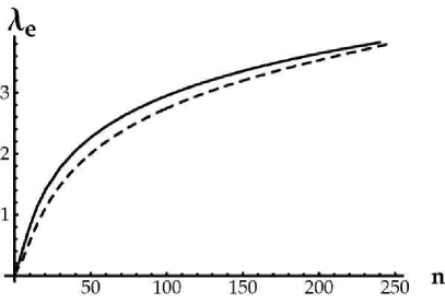
Figure 1: Eigenvalues of electrostatic energy matrix calculated from Eq. (6), at $L/b=1000$ and $\kappa L=10$ (dashed curve), compared to the eigenvalues calculated in the infinite length limit in Eq. (14) (solid curve).

The electrostatic energy comprises one portion of the total energy of the semiflexible PE. The other contribution arises from the elastic modulus, quantified by the “bare” persistence length, $\ell_{p0}$ and appearing in the energy as the first term on the right-hand side of Eq. (1). The large eigenvalues of the matrix ${\bf T}$ are dominated by the diagonal terms $(n\pi)^{2}(\ell_{p0}/L)$ in, for instance, the right-hand side of Eq. (5). Thus, the effect of electrostatic interaction is more pronounced on the lower eigenvalues, while it is swamped by semiflexible energetics at short length scales. In Fig. 2, the eigenvalues of the total Hamiltonian are compared with the bending eigenvalues. Only the first few eigenvalues are distinguishable from each other. The value of $n$ for which the electrostatic effects can be neglected depends on the strength of electrostatic interaction $\beta L$ and the intrinsic persistent length.

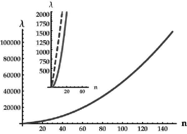
Figure 2: Eigenvalues of an elastic charged rod with $\ell_{p0}/L=0.5$, $\kappa L=0$, and $\beta L=500$. The bending eigenenergies are distinguishable from total ones only for lower values of $n$. Comparison of the first 20 eigenvalues of bending (solid line) and total (dashed line) eigenvalues could be seen in the inset.

The general behavior of the larger eigenvalues associated with “pure” electrostatic energy, which grow logarithmically with index, $n$, is fundamentally different from those resulting to “pure” elastic energy, which grow quadratically with index. In the case of a neutral polymer with an intrinsic persistence length that is comparable with the total length of polymer, the series in Eq. (13) converges very rapidly, as noted in Ref. Wilhelm and Frey (1996). When the chain is charged, and especially when the persistence length is due predominantly to electrostatic effects, more terms in the series Eq. (13) must be preserved in order to obtain a stable answer for $G(r)$. In our calculation, the matrix ${\bf T}$ is truncated at a size much greater than the number of terms needed to obtain an accurate answer for the series in Eq. (13). There are two reasons for this. First, the greater the dimension of the truncated matrix, the more accurate are the values of lower eigenvalues which participate in the sum. Second, retaining more terms in the product on the right-hand side of Eq. (12) helps us achieve a higher accuracy in our result for the function $f(n)$. In practice, we increased the dimension of the matrices until the effect (on the end-to-end distribution function) of a further increase in the size of ${\bf T}$ by a factor of four was less than a part in a thousand.

The truncation of the matrices above is also related to the short distance cutoff $b$. The dimensions of these matrices should not be larger than $L/b$. This is because matrices corresponding to a cosine basis set for which the wavenumber is greater than $1/b$ are influenced by features at length scales shorter than $b$, and such features are inconsistent with the inherent coarse-graining in our energy expression. We determine the truncation of matrices by looking for convergence of the numerical procedure, as noted above. We then check to see that the size, $N$, of the basis set satisfies $N\leq L/b$. At no point in our calculations was this inequality violated.

As $r\rightarrow 1$, the dimension of the matrices must be very high in order to obtain reliable answers. It is possible to calculate the integral in Eq. (10) numerically without performing contour integration. This method is very time-consuming but it is more reliable because this way we reduce significantly the roundoff error caused by the sum in Eq. (13). We used this approach for very large values of $\beta L$.

III.2 Exact Analytical Eigenfunctions and Eigenvalues of the Unscreened Coulomb Interaction Energy

Although we are not able to produce exact, analytical solutions to the eigenvalue equations of the quadratic weight in Eq. (6), for arbitrary values of the inverse screening length, $\kappa$, it has proven possible to obtain the eigenfunctions and eigenvalues of the unscreened version of the energy operator. The results of the analytical investigation provide a check for our numerics and provide insight into the qualitative behavior of eigenfunctions and eigenvalues of the energy operators controlling the conformational statistics of rod-like PE’s.

As it turns out, the investigations of the properties of the operator in this special case is most conveniently carried out in “real space”—that is, with arc-length, $s$, as the independent variable. In this section, we will summarize the methods utilized and the results obtained in this investigation. The details of the calculation are presented in Appendix B. The key result is that the eigenfunctions of the unscreened Hamiltonian have the form

$$\xi_{k}(s)=s^{-1/2}\sin\left(k\ln\frac{s}{b}+\phi(k)\right)$$ (15)

and that the eigenvalues are given by

$$\lambda(k)=\Lambda\left(-\frac{1}{2}+ik\right)$$ (16)

where the function $\Lambda(p)$ is defined in Eq. (32). When the dimensionless wave-vector-like quantity, $k$, is large, the eigenvalues are essentially linear in $\ln k$. This is to be expected, given the form of the unscreened Coulomb interaction, and is, in fact, consistent with our numerical results.

We can now attempt a comparison between the expressions for the eigenfunctions in Eq. (15), and eigenvalues in Eq. (16), and the numerically generated eigenfunctions and eigenvalues of the unscreened energy operator whose matrix elements in the cosine basis are given in Eq. (6). The eigenvalues are compared in Fig. 3, and a comparison for a low-lying eigenvector is displayed in Fig. 4. As indicated by the figures, the numerical correspondence is excellent. The quality of the comparison serves as a validation of the numerical calculations carried out here.

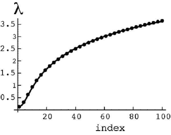
Figure 3: Comparison of the eigenvalues $\lambda(k)$ as given by Eq. (34) with the numerical eigenvalues of the unscreened Coulomb energy matrix as given by Eq. (6). As indicated in the figure, the horizontal axis is the index of the eigenvalue. The formula (34) is the solid curve, passing through the filled circles, which indicate the location of the eigenvalues of the discrete version of the operator in Eq. (6). To facilitate the visual comparison, the numerical eigenvalues have been “thinned out,” in that every third numerical eigenvalue is shown.

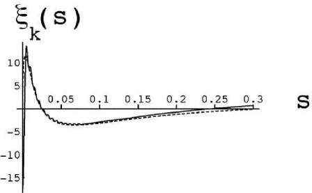
Figure 4: Comparison of the numerically determined eigenvector of the discrete version of the Coulomb energy kernel associated with the sixth-lowest eigenvalue (solid curve) and of the eigenfunction generated by the formula (15) (dashed curve). The value of the parameter $k$ in that formula is adjusted to optimize the fit between the two curves, with the use of a least-squares procedure. The actual value of $k$ used here is 1.3. The oscillations in the solid curve are the result of the cutoff in the cosine basis set.

It is possible to assess the importance of a small term representing the influence of “pure” bending energy, by treating that term as a perturbation of the overall energy of the polyelectrolyte chain. At first order in perturbation theory, a straightforward calculation leads to the following result for the ratio of the pure bending energy contribution to the eigenvalue to the zeroth order energy resulting from an unscreened Coulomb interaction

$$\frac{E_{\rm bending}}{E_{\rm Coulomb}}=\frac{l_{p0}\left[(1+4k^{2})/4\right]\left[k^{2}/(1+k^{2})\right]}{2l_{B}\lambda(k)\ln(L/b)}$$ (17)

Note that in the limit of an infinitely long polyelectrolyte chain, the unscreened Coulomb interaction always dominates. The divergence in the denominator as $L\rightarrow\infty$ is, however, quite slow. As practical matter, the bending energy due to the intrinsic cost of introducing curvature into a semi-flexible chain will eventually overcome the Coulomb energy as a contribution to the conformation energy of the chain. In light of this fact, one can obtain results for the end-to-end distribution of an unscreened chain in the presence of a bending energy.

In this regard, it should be noted that in the absence of a bending energy, the expression (10) for the end-to-end distribution of an unscreened polyelectrolyte chain is formally divergent. This is because of the very slow increase in the eigenvalues (16) as a function of $k$. A full investigation of the conformational statistics of the unscreened polyelectrolyte chain has not yet been carried out, and will in all probability yield surprises.

IV Radial Distribution Function of Polyelectrolytes

Using the eigenvalues of the effective Hamiltonian for the rodlike PE, we can calculate the radial distribution function from Eq. (13). Figure 5 illustrates the effect of the screened electrostatic interaction on the distribution function of a neutral chain (dashed line), for three different values of $\kappa L=12$, $\kappa L=6$ and $\kappa L=3$. $\beta L=100$ for the three PE distributions. As manifested in the figure, the distribution function of the polyelectrolyte has shifted toward larger extensions and is peaked more sharply around the maximum compared to the neutral chain. Upon decreasing the screening length, the monomer-monomer repulsion becomes more strongly screened and the distribution function of the end-to-end distance peaks towards shorter extensions.

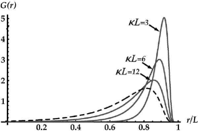
Figure 5: Comparison of distribution function of polyelectrolytes for $\kappa L=12$, $\kappa L=6$ and $\kappa L=3$, respectively from left to right.

To construct a quantitative measure for the elasticity of polyelectrolytes, we investigate to what degree and under what conditions the radial distribution function of a polyelectrolyte can be reproduced by the distribution of a neutral chain with an adjusted persistence length. To this end, we attempt to collapse the distribution function of a polyelectrolyte onto the distribution function of a wormlike chain with an effective $\ell_{p}$, and observe that the answer to the above question depends on the values of $\ell_{p0}/L$, $\kappa L$ and $\beta L$.

We investigate the effects of overall charging of the chain as quantified by the combination $\beta L$, of the screening length, equal to $\kappa^{-1}$, of the length of the chain, $L$ and of the chain’s intrinsic stiffness, described in terms of the bare persistence length, $\ell_{p0}$. We are able to identify regimes in which the conformational statistics of a rod-like PE is effectively indistinguishable from that of a neutral WLC, and we also find that there are regions in parameter space in which the radial distribution of a charged semiflexible rod-like chain cannot be reproduced by the corresponding distribution of a neutral chain.

Our conclusions are summarized in the four subsections below. Briefly, we find that sufficiently strong charging, a sufficiently long screening length, sufficiently short overall chain length or sufficiently weak intrinsic stiffness can give rise to deviations between the conformational statistics of a PE and that of a WLC.

IV.1 Effect of Electrostatic Charging

There is a substantial regime in the parameter space in which the distribution of a polyelectrolyte matches exactly that of a wormlike chain with an adjusted persistence length, particularly when the electrostatic interaction plays a perturbative role in the chain energetics. There are also regimes in which the electrostatic interaction gives rise to a substantial portion of the stiffening energy, and in which the radial distribution of the PE is the same as that of a neutral WLC. For a sufficiently strong electrostatic interaction, however, the polyelectrolyte distribution begins to deviate from the wormlike chain form. This is illustrated in Fig. 6 where the polyelectrolyte distribution is compared with that of the best effective wormlike chain description for the two cases of low and high charging. It is clear that at strong enough charging, the electrostatic energy establishes the conformational statistics.

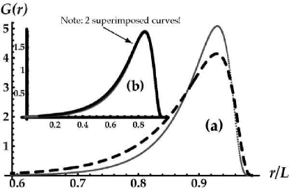
Figure 6: (a) The distribution for a polyelectrolyte with $\ell_{p0}=0.5$, $\beta L=600$, and $\kappa L=10$, compared to that of a wormlike chain with $\ell_{p}=1.3$. Inset: (b) The distribution for a polyelectrolyte with $\ell_{p0}=0.5$, $\beta L=60$, and $\kappa L=10$, compared to that of a wormlike chain with $\ell_{p}=0.6$ (two superimposed curves).

IV.2 Effect of Electrostatic Screening

The degree of screening of the electrostatic interaction similarly affects the form of the end-to-end distribution. In the high-ionic-strength regime it is possible to obtain a satisfactory match of the polyelectrolyte distribution with that of an effective wormlike chain. However, as screening decreases, the polyelectrolyte distribution deviates significantly from the wormlike chain form. Comparison of Figs. 6(a) and 7 illustrates the difference between high and low screening for a given intrinsic stiffness and charging. We observe that as we increase screening, the two distribution collapse on top of each other.

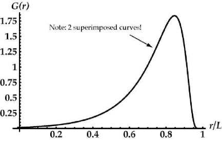
Figure 7: The distribution for a polyelectrolyte with $\ell_{p0}=0.5$, $\beta L=600$, and $\kappa L=50$, compared to that of a wormlike chain with $\ell_{p}=0.56$ (two superimposed curves).

Our calculations verify that under physiological conditions ($\kappa=1\ {\rm nm}^{-1}$), the distribution functions for rod-like DNA segments ($L\raisebox{-2.168pt}{$\stackrel{{\scriptstyle<}}{{\sim}}$}100\ {\rm nm}$) as well as those of stiffer actin filaments also collapse onto the end-to-end distribution for neutral chains with an effective persistence length given by Eq. (18).

IV.3 Effect of Finite Length

In most of the studies of the elasticity of polyelectrolytes that have been carried out to this point, the finite length of the polyelectrolyte and the corresponding end-effects have been assumed to be unimportant. We have re-examined this assumption by considering two sets of parameters that correspond to identical values for $\ell_{p0}$, $\beta$, and $\kappa$, and different values for the contour length $L$ of the polyelectrolytes. As can be seen in Fig. 8, while the distribution for longer chains can be satisfactorily collapsed onto that of a wormlike chain, the situation is completely different for shorter chains. This highlights the importance of end effects in the elasticity of polyelectrolytes.

It is important to note that a rescaling of the backbone length of the PE is not an acceptable stratagem for improving the agreement between the PE radial distribution and that of a WLC. This is because the backbone length is essentially fixed by the rod-like chain condition. The shortening and thickening that is associated with intermediate blob-like structures Khokhlov (1980) will not occur. In fact, we have observed that a reduction in the effective value of $L$ actually degrades the quality of the correspondence between the conformational statistics of a PE and those of the corresponding WLC. In general, our calculations indicate that the difference between the radial distribution of the PE and the WLC is partly due to the influence of end effects. A complete investigation of these effects is described in Ref. Zandi et al. (a).

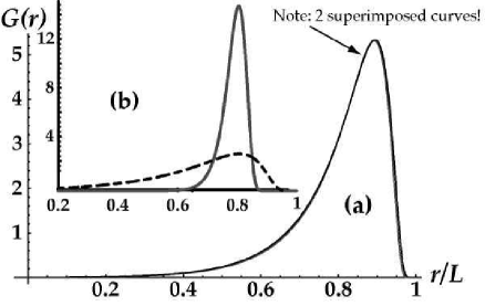
Figure 8: (a) The distribution for a polyelectrolyte with $\ell_{p0}/L=0.0001$, $\beta L=36000$, and $\kappa L=100$, compared to that of a wormlike chain with $\ell_{p}=0.87$ (two superimposed curves). Inset: (b) The distribution for a polyelectrolyte with $\ell_{p0}/L=0.01$, $\beta L=360$ and $\kappa L=1$, compared to that of a wormlike chain with $\ell_{p}=0.565$. The difference between the two sets of parameters is only in the length of the chain.

IV.4 Effect of Intrinsic Stiffness

Fig. 8(b) indicates that for $\kappa L=1$ and $\beta L=360$ when the intrinsic persistence length of a chain is small ($\ell_{p0}\ll L=0.01$), the radial distribution function of a polyelectrolyte does not exhibit near-perfect matching with that of an uncharged wormlike chain . In this almost unscreened case, matching is achieved, when the chain becomes sufficiently stiff. If $\ell_{p0}/L$ is increased to 35, while $\kappa L$ remains equal to one and $\beta L=360$, the radial distribution of a PE will be indistinguishable from the corresponding distribution of a neutral WLC with a persistence length $\ell_{p}=39L$. The fact that such a large intrinsic persistence length is required to achieve this kind of matching of the two distribution highlights the importance of electrostatic interactions in this case.

IV.5 Applicability of the WLC Model: A General Diagram

The effects discussed above can be summarized in a general diagram in the three dimensional parameter space. This diagram, shown in Fig. 9, illustrates the conditions under which a WLC model provides an accurate description of the conformational statistics of a short, rod-like PE. The lines shown indicate the locations of the crossover regions that separate the regime in which one can think of a short segment of a PE as a WLC with a modified persistence length from the regime in which the statistics of a PE is fundamentally distinct from that of a WLC.

As can be seen in Fig. 9, for a given value of the screening parameter, charging up the PE will cause a crossover from WLC into non-WLC behavior. This crossover is, however, hampered by increased intrinsic stiffness.

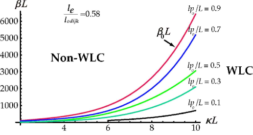
Figure 9: The diagram delineating the regimes in which the statistics of a rod-like PE is the same as that of a WLC with a suitably modified persistence length from the regimes in which the statistics of the two models are fundamentally different. The curves separating the two regimes correspond to $\ell_{e}/\ell_{\rm Odijk}=0.58$ for various values of $\ell_{p0}/L$. These lines also indicate the values of $\beta_{0}L$ in Eq. (19) at different values of $\kappa L$ and $\ell_{p0}/L$. No curves were drawn outside of the range of rodlike behavior. For this reason, the curves for $\ell_{p0}/L=0.1$ and $\ell_{p0}/L=0.3$ are truncated.

V Electrostatic Persistence Length

In this Section, we investigate the concept of the electrostatic persistence length. As in the previous section, we will find that there are regimes in which Odijk’s formula [Eq. (18] below) for the effective persistence length of a PE Odijk (1977) is accurate, and that there are regimes in which it does not hold. As it turns out, there is a strong correlation between the accuracy of this formula and the correspondence between PE and neutral WLC conformational statistics. When the radial distribution function of a PE is well-reproduced by that of a neutral WLC, the persistence length of the corresponding WLC is accurately predicted by Odijk’s formula. Conversely, when the two distributions do not collapse on one another, the persistence length of the “best-fit” WLC is not predicted by that formula.

We have seen in Sec. IV that one can collapse the distribution function of a polyelectrolyte onto the distribution function of a wormlike chain with an adjusted persistence length whenever the Coulomb interaction is no more than a perturbation to the mechanical stiffness of the chain, or when Debye screening is sufficiently strong. In these regimes, the persistence length of the neutral chain follows Odijk’s prediction, in that, $\ell_{p}=\ell_{e}+\ell_{p0}$, where $\ell_{p}$ is the effective persistence length of the charged chain, and the electrostatic persistence length $\ell_{e}$ is given as Odijk (1977)

$$\ell_{\rm Odijk} = \frac{\beta L^{2}}{12}\left[e^{-\kappa L}\left(\frac{1}{\kappa L}+\frac{5}{(\kappa L)^{2}}+\frac{8}{(\kappa L)^{3}}\right)\right.$$ (18)

$$\left.+\frac{3}{(\kappa L)^{2}}-\frac{8}{(\kappa L)^{3}}\right],$$

which reduces to $\ell_{\rm OSF}\equiv\beta/4\kappa^{2}$ for large $\kappa L$ Odijk (1977); Skolnick and Fixman (1977). For instance, at $\beta L=600$ and $\kappa L=50$, if we add $\ell_{\rm OSF}=0.06$ to $\ell_{p0}=0.5$, we find $\ell_{p}=0.56$. The distribution function of this polyelectrolyte collapses perfectly onto that of a wormlike chain with $\ell_{p}=0.56$. It is important to note that the expression for $\ell_{\rm Odijk}$ was derived under the assumption that $\ell_{p0}\sim L$, the contour length of the chain, $L$, is of the order of its intrinsic persistence length, $\ell_{p0}$ and that the electrostatic interaction has the limited effect of “perturbing” the wormlike chain shape of the chain Odijk (1977). Our results confirm the validity of OSF formula in the regime in which it is expected to be correct ($\kappa L\gg 1$).

For long chains, substantial charging is required in order to enforce the rodlike limit. It is important to note that despite the substantial charging of the chain, the ratio of the length of the PE to the screening length, $\kappa L$, must be sufficiently large. This requirement is essential in order to minimize the strong influence of the end effects on conformational statistics of charged chains.

The important characteristic of this regime is that $\ell_{p0}\ll\ell_{e}$ and thus electrostatic energy no longer plays a perturbative role. However, we find that in this regime Odijk’s formula works perfectly well as well, provided the screening is strong enough. For example, at $\ell_{p0}/L=0.0001$, $\beta L=36000$, and $\kappa L=100$, we find $\ell_{e}/L=0.87$ which is a near-perfect match with $\ell_{\rm Odijk}$ (see Fig. 8). The accuracy of Odijk’s formula when $\ell_{e}\gg\ell_{p0}$ is not at all obvious, as OSF was derived in the regime where electrostatic interaction plays a perturbative role.

We emphasize that the reason for the high quality of the match with OSF in this regime is different from the reason for the corresponding result obtained by Khokhlov and Khachaturian Khokhlov and Khachaturian (1982) for weakly charged flexible chains. In our case, the chain is stiff in all length scales; the possibility of renormalizing the length and/or charge is thus excluded in our formulation.

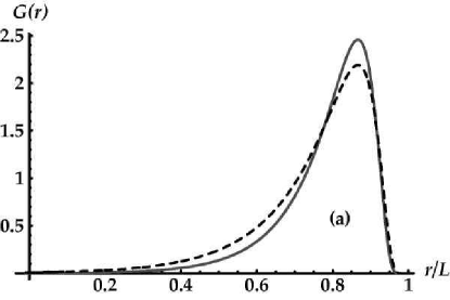
Figure 10: The intrinsic persistence length of the charged chain is $\ell_{p0}/L=0.5$, $\beta L=45$ and $\kappa L=2$. The persistence length of the wormlike chain is $\ell_{p}/L=0.767$.

As noted in Sec. IV, increasing the electrostatic coupling or screening length, one encounters a regime in which it is no longer possible to obtain near-perfect collapse of the polyelectrolyte distribution onto that of an effective wormlike chain. Figure 10, displays the polyelectrolyte end-to-end distribution (solid curve) along with the modified wormlike chain distribution (dashed curve) in a case in which it is possible to obtain a good, but not perfect fit. The fit was obtained by matching the location of the maxima of the two distributions, and the electrostatic persistence length attributed to the polyelectrolyte distribution is that of the wormlike chain associated with the dashed curve. The PE distribution shown in the figure matches the result of computer simulation of a rodlike PE Netz . In this case the ratio of electrostatic persistence length extracted from the distribution function to Odijk’s persistence length is, $\ell_{e}/\ell_{\rm Odijk}=0.58$. As noted at the beginning of this section, the more the two distributions are different from each other, the more the effective persistence length of the polyelectrolyte deviates from the Odijk’s prediction. For example, The persistence length of the wormlike chain shown in Figure 8 (b) is $\ell_{p}=0.565$, while the effective persistence length of the polyelectrolyte according to Odijk is $\ell_{p0}+\ell_{\rm Odijk}=4.52$. The two distributions differ significantly and the ratio is $\ell_{e}/\ell_{\rm Odijk}=0.12$.

Our general observation is that the ratio of $\ell_{e}$ extracted from the effective wormlike chain distribution to Odijk’s persistence length correlates with the quality of the fit of an effective wormlike chain end-to-end distribution to that of a polyelectrolyte. When this ratio is equal to one, the polyelectrolyte can be completely described in terms of a wormlike chain. As this ratio decreases, the deviation becomes more pronounced. Figure 9 displays a diagram, which delineates the quality of the fit. The line that is used in the Figure to separate the two regimes corresponds to $\ell_{e}/\ell_{\rm Odijk}=0.58$. As indicated in this Figure (and described in Sec. IV.5), for fixed $\kappa L$, when $\beta L$ is below a certain value the polyelectrolyte behaves like a wormlike chain, while for larger $\beta L$ the two distributions start to differ significantly. This crossover scale is sensitive to the intrinsic flexibility of the PE, as shown in Fig. 9.

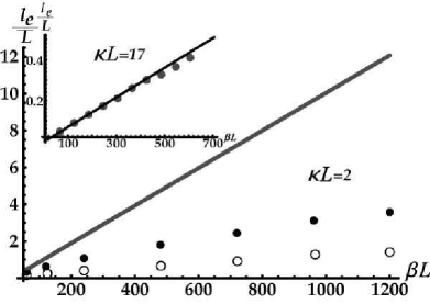
Figure 11: Comparison of our results for the electrostatic persistence length with Odijk’s finite size formula (solid line) at $\kappa L=2$ with $\ell_{p0}/L=0.5$ (filled circles) and $\ell_{p0}/L=0.01$ (hollow circles). The inset is for $\kappa L=17$ and $\ell_{p0}/L=0.5$.

There is a substantial difference between the electrostatic persistence length of a rodlike polyelectrolyte and Odijk’s prediction as we increase the electrostatics strength $\beta L$. As illustrated in Fig. 11, the deviation of $\ell_{e}/L$ from $\ell_{\rm Odijk}/L$, with increasing $\beta L$ is more pronounced at lower values of $\kappa L$. At $\kappa L$=17, this deviation becomes evident when $\beta L\sim 1000$. However, at $\kappa L=2$, the deviation is evident already when $\beta L\sim 30$.

A review of the current literature on elasticity of polyelectrolytes reveals that there is no simple theory for computing $\ell_{e}$ with arbitrary intrinsic stiffness. It is generally believed that as long as a polyelectrolyte chain is stiff, the dependence of $\ell_{e}$ on $\kappa$ is correctly given by the OSF formula. However, our results indicate that in certain regimes the electrostatic persistence length, $\ell_{e}$, depends on $\ell_{p0}$, and is smaller than is predicted by the OSF formula. Figure  11 shows that the electrostatic persistence length of a rodlike polyelectrolyte, $\ell_{e}/L$, depends on $\ell_{p0}/L$. This dependence is not present in Odijk’s formula.

Our general observation of the curves of $\ell_{e}$ versus $\beta L$ is that they asymptote to a power law of the form $\ell_{e}\propto(\beta L)^{x}$ where the exponent $x(\kappa L)$ is less than $1$. This behavior has been predicted by Barrat and Joanny with an exponent $x=1/2$ in the limit $\beta L\to\infty$ Barrat and Joanny (1993). We find, however, that the asymptotic limit is approached much more slowly than it is predicted by the Barrat-Joanny crossover formula. The section below describes our attempt to systematize the relationship of the effective persistence length to Odijk’s prediction ita .

VI Universal Behavior

In search of a possible universal pattern which might relate $\ell_{p0}/L$, $\beta L$ and $\kappa L$ to $\ell_{e}$, we have rescaled our graphs for different values of the parameters. To this end, we choose a value of $\beta$ called $\beta_{0}$ such that $\ell_{e}/\ell_{\rm Odijk}=0.58$, and rescale the parameter $\beta$ with it, where the value of 0.58 is completely arbitrary. We have followed this procedure to rescale our graphs for different values of $\kappa L$, keeping $\ell_{p0}/L$ constant. Figure 12 contains these rescaled graphs for $\kappa L=6,8,10,12$, which collapse satisfactorily on top of each other. It is important to note that when we choose any other ratio of $\ell_{e}/\ell_{\rm Odijk}$ to rescale our graphs, we obtain the same universal behavior among our curves. The solid line in Fig. 12 corresponds to the following crossover or interpolation formula for $\ell_{e}$

$$\ell_{e}=\frac{\ell_{\rm Odijk}}{1+c(\beta/\beta_{0})^{x}},$$ (19)

plotted with the exponent $x=0.4$. In the above equation, $c=0.724$ is constant which ensures the ratio of $\ell_{e}/\ell_{\rm Odijk}$ for a given value of $\beta_{0}$.

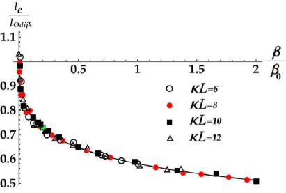
Figure 12: Comparison of our data, suitably rescaled, to the expression in Eq. (19) for the form of the correction to Odijk’s formula for the electrostatic persistence length. The points correspond to our rescaled plots of $\ell_{e}/L$ versus $\beta L$ at $\kappa L=6,8,10,12$.

As exemplified in Fig. 12, this formula provides a remarkable fit to our data. To calculate the exponent $x$, we have attempted to fit our curves of $\log(\ell_{\rm Odijk}/\ell_{e}-1)$ versus $\log(\beta/\beta_{0})$ to a straight line. As shown in Fig. 13, all our data are fitted to a straight line with slope approximately equal to 0.4. Similar curves have been generated for other, smaller, values of $\ell_{p0}/L$. The behavior of these other curves is the same as the one plotted in Fig. 12.

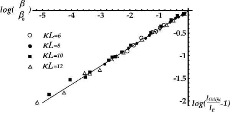
Figure 13: Demonstration of the universal scaling behavior for $\ell_{e}$. The points correspond to our rescaled plots of $\ell_{e}/L$ versus $\beta L$ at $\kappa L=6,8,10,12$. The equation of straight line is $y=0.006+0.401x$.

The quantity $\beta_{0}$ is an increasing function of $\ell_{p0}$ and $\kappa$. We have been able to obtain the value of $\beta_{0}$ from our data. The crossover discussed in the previous section occurs when $\beta=\beta_{0}$ which corresponds to $\ell_{e}\simeq 0.58\ell_{\rm Odijk}$ in Eq. (19). Hence, the curves in Fig. 9 indicate the values of $\beta_{0}L$ for different values of $\kappa L$ and $\ell_{p0}/L$. The dependence of $\beta_{0}$ on the parameters $\ell_{p0}$, $\kappa$, and $L$ seems to be in general quite complicated. For $\ell_{p0}\kappa>1$, we seem to find that $\beta_{0}\sim L^{2}\kappa^{4}\ell_{p0}\;g(\kappa L)$, where $g$ is a polynomial function. For $\ell_{p0}\kappa<1$, however, the leading dependence on $\kappa$ seems to be a much stronger power law. We are still investigating the dependence of $\beta_{0}$ on the parameters in all the different regimes Zandi et al. (b).

VII First and Second Moments of the Distribution

Much theoretical work on electrostatic persistence length, is based on the calculation of $\langle r\rangle$ or $\langle r^{2}\rangle$ of a polyelectrolyte. Odijk uses the second moment to test the validity of OSF when $\ell_{e}>\ell_{p0}$ Odijk (1977). It is thus crucial to learn to what extent the conformational statistics of polyelectrolytes are similar to those of wormlike chains when they share the same $\langle r\rangle$ or $\langle r^{2}\rangle$. It is not obvious that the matching of first or second moments of the end-to-end distribution will yield the matching of the higher moments of the distribution as well.

We extract an “effective” persistence length by matching the first or second moments of the end-to-end distance of a polyelectrolyte distribution with that of an effective wormlike chain in order to compare our results with other existing theories.

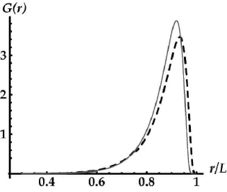
Figure 14: The taller distribution (solid line) belongs to a polyelectrolyte at $\kappa L=17$, $\ell_{p0}=0.5$ and $\beta L=1000$. The shorter distribution (dashed line) is adjusted so that its second moment is the same as that of the polyelectrolyte distribution.

Figure 14 contains the end-to-end distribution function for a screened polyelectrolyte with $\kappa L=17$, $\ell_{p0}/L=0.5$ and $\beta L=1000$ along with the distribution function of an uncharged wormlike chain with $\ell_{p}/L=1.22$. The shorter distribution is adjusted so that its second moment is the same as that of the polyelectrolyte distribution. It is noteworthy that the persistence length of the uncharged wormlike chain agrees perfectly well with Odijk’s prediction, while the two distribution functions are distinguishable from each other. In general, we observe that the maximum of the wormlike chain distribution is shifted toward larger extension when we match $\langle r^{2}\rangle$ of the two distributions as exemplified in the Figure.

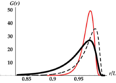
Figure 15: The thin solid line is the plot of $G(r)$ for a polyelectrolyte with $\beta L=600$, $\kappa L=0$, and $\ell_{p0}/L=0.5$. The thick solid line with $\ell_{p0}/L=3.1$ belongs to a WLC distribution for which its maximum is matched to that of the PE distribution. The dashed plot is for a neutral chain with $\ell_{p0}/L=4.86$. The dashed distribution and polyelectrolyte have the same first moment.

Similar results are observed when we match the first moment of distribution of a polyelectrolyte with that of a wormlike chain with an adjusted persistence length. In Fig. 15, the distribution function of a polyelectrolyte along with two distribution functions for effective wormlike chains is presented. The dashed line and polyelectrolyte share the same first moment. As illustrated in the Figure, the two distributions differ significantly.

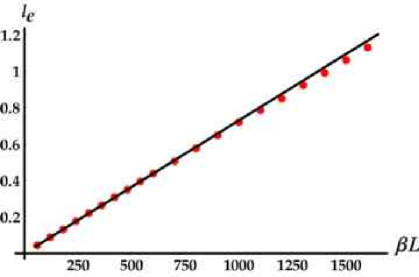
Figure 16: Comparison of our results for the electrostatic persistence length with Odjik’s finite size formula [ Eq.(18)] (solid line) at $\kappa L=17$. Our numerical results are based on matching of the second moment of distributions.

We have compared the electrostatic persistence length given in Eq. (18) with our results obtained by matching $\langle r^{2}\rangle$ of a PE distribution to that of a WLC distribution. Figure 16 shows that for $\kappa L=17$, our data begins to deviate from Odijk’s finite size formula when $\beta L\sim 1200$.

It is important to note that when we match the maximum of distributions to extract an effective persistence length, the deviation from Odijk’s prediction begins at $\beta L\sim 400$ for $\kappa L=17$ (the inset in Fig. 11). This is the point when the two distributions cease to closely resemble each other. However, if we use the matching of the first or second moment to calculate the effective persistence length, the two distributions would clearly be distinguishable from each other well within the regime in which Odijk’s formula for the persistence length remained accurate.

This points to the fact that replacing a PE chain by a WLC, when they share the same $\langle r^{2}\rangle$ or $\langle r\rangle$, is not well-justified in all regimes and that one should use care in the utilization of the notion of an electrostatic persistence length based on matching of first or second moments.

VIII Conclusion

The difficulty in producing a complete characterization of the mechanical properties of a charged, semiflexible chain arises from the existence of a number of length scales in that system. In particular, it is far from clear that the notion of a persistence length provides an adequate description of the mechanical and thermal characteristics of such a chain. In light of this, the end-to-end distribution function provides an attractive alternative. Given that the distribution is a function, rather than a single number, it represents considerably more information about the charged chain.

One important application of this distribution is in the assessment of the utility of the notion of a persistence length, in that it is possible to compare the distribution obtained experimentally, via simulations, or as the result of explicit calculations, with the corresponding distribution of a neutral semiflexible chain. On the basis of explicit calculations, we have been able to determine the extent to which the end-to-end charged chain can be collapsed onto the end-to-end distribution of a neutral worm-like chain with an adjusted persistence length. Among the regimes in which this correspondence is achieved are those in which electrostatic effects play a perturbative role. In addition to collapse of the two distributions in these regimes, we also find that the electrostatic persistence length is given by the formulas of Odijk and OSF. This result is consistent with the assumptions underlying those formulas. We also observe collapse of the distributions and can verify the validity of the Odijk and OSF results for the effective persistence length in regimes in which the charging of the chain is sufficiently strong that electrostatic effects dominate purely mechanical energetics as long as Debye screening of electrostatic interactions is sufficiently strong.

In fact, we find that there is a strong correlation between correspondence of the distributions of charged and uncharged chains and the validity of Odijk’s formula for the effective persistence length. When the distributions can be collapsed onto each other, the formula proves to be accurate, while lack of correspondence of the two distributions is accompanied by inaccuracy of the Odijk result for the effective persistence length. Our results indicate that the difference between the radial distribution of the PE and the WLC can be attributed, at least in part, to the influence of end effects. In fact, we believe that the behavior of the persistence length is substantially controlled by end effects. One way of understanding this is in terms of Odijk’s derivation of the expression (18) for the electrostatic persistence length Odijk (1977). This derivation is based on a calculation of the energy of a bent segment of a charged rod. A key assumption in this derivation is that the segment takes the form of an arc of a circle. End effects are readily associated with the difference between the shape of a real bent rod and the circular arc assumed in Odijk’s derivation. An exploration of these effects in this context is described in Ref Zandi et al. (a).

Another important finding is that an effective persistence length, obtained by locating the maximum of the distribution, can be described in terms of a scaling formula, Eq. (19). This formula relates the actual persistence length to the Odijk predictions. The formula is “universal,” in that it has a general form that is independent of the parameters utilized, and it incorporates a power law that does not appear to be anticipated in the Hamiltonian governing the system, nor does it arise from any simple dimensional analysis. At this point, we have no explanation for either the universal form or the power law.

As noted above, the effect of counterion condensation has been ignored throughout the above work. It has been shown that counterion condensation modifies the bending rigidity of a semiflexible chain Golestanian et al. (1999); Stevens and Kremer (1995); Rouzina and Bloomfield (1998); Diamant and Andelman (2000) and may result in the collapse of the PE chain Golestanian et al. (1999). We have performed a calculation of the distribution function taking into account the attractive interaction due to counterion fluctuations and observed the signature of collapse. In general, one is able to observe the collapse of a charged chain for any strong enough attractive interaction which is in function of the distance between monomers. We are currently investigating these effectsZandi et al. (b).

Appendix A Expansion of the Coulomb Interaction

In this Appendix, the expansion of the Coulomb self-interaction for a charged chain that is slightly deformed about the rodlike configuration is derived. Using Fourier representation of the screened Coulomb interaction we find

$$\int_{0}^{L}ds\int_{0}^{L}ds^{\prime}\frac{e^{-\kappa|{\bf r}(s)-{\bf r}(s^{\prime})|}}{|{\bf r}(s)-{\bf r}(s^{\prime})|} = \int\frac{d^{3}{\bf k}}{(2\pi)^{3}}{4\pi\over k^{2}+\kappa^{2}}\int_{0}^{L}ds\int_{0}^{L}ds^{\prime}\;\exp\left\{i{\bf k}\cdot\left[{\bf r}(s)-{\bf r}(s^{\prime})\right]\right\}$$ (20)

$$\simeq \int\frac{d^{3}{\bf k}}{(2\pi)^{3}}{4\pi\over k^{2}+\kappa^{2}}\int_{0}^{L}ds\int_{0}^{L}ds^{\prime}\;\exp\left\{i{\bf k}_{\perp}\cdot\int_{s}^{s^{\prime}}du\;{\bf a}(u)-{ik_{z}\over 2}\int_{s}^{s^{\prime}}du\;{\bf a}(u)^{2}+ik_{z}(s^{\prime}-s)\right\}$$

$$= \int\frac{d^{3}{\bf k}}{(2\pi)^{3}}{4\pi\over k^{2}+\kappa^{2}}\int_{0}^{L}ds\int_{0}^{L}ds^{\prime}\;e^{ik_{z}(s^{\prime}-s)}$$

$$\;\times\;\left[1-{1\over 2}\left({\bf k}_{\perp}\cdot\int_{s}^{s^{\prime}}du\;{\bf a}(u)\right)-{ik_{z}\over 2}\int_{s}^{s^{\prime}}du\;{\bf a}(u)^{2}+O(a^{3})\right].$$

Appendix B General form of the energy associated with distortions of a rod-like polyelectrolyte stiffened entirely by unscreened Coulomb interactions

Suppose that the tangent vector ${\bf t}(s)$ is as given by Eq. (4). Suppose, also, that the interaction energy of the rod-like polyelectrolyte is given by

$${\cal E}=\frac{\beta}{2}\int_{0}^{L}ds\int_{0}^{L}ds^{\prime}V(\textbf{r}(s)-\textbf{r}(s^{\prime})).$$ (21)

Making use of Eq. (4) and the relationship

$$\textbf{r}(s)=\int_{0}^{s}\textbf{t}(s_{1})ds_{1},$$ (22)

and expanding to the resulting expression for the energy ${\cal E}$ to second order in the deviation, $\textbf{a}(s)$, from a straight line in th $z$-direction, we find that the energy is given by

$${\cal E} = \frac{\beta}{2}\left\{\int_{0}^{L}ds\int_{0}^{L}ds^{\prime}V(s-s^{\prime})\right.$$ (23)

$$\left.+\int_{0}^{L}ds\int_{0}^{L}ds^{\prime}{\cal K}(s,s^{\prime})\textbf{a}(s)\cdot\textbf{a}(s^{\prime})\right\},$$

where

$${\cal K}(s,s^{\prime})=\delta(s-s^{\prime})\int_{0}^{L}{\cal L}(s,s^{\prime})ds^{\prime}-{\cal L}(s,s^{\prime}),$$ (24)

and

$${\cal L}(s,s^{\prime})=-\int_{0}^{s_{<}}ds_{a}\int_{s_{>}}^{L}ds_{b}\frac{V^{\prime}(s_{b}-s_{a})}{s_{b}-s_{a}},$$ (25)

and $s_{>(<)}$ is the greater (smaller) of $s$ and $s^{\prime}$. If the charges on the polyelectrolyte interact via the unscreened Coulomb potential, then the interactions leading to the kernel ${\cal L}(s,s^{\prime})$ are straightforward, and we find

$${\cal L}(s,s^{\prime})=\frac{1}{2}\left[\frac{1}{s_{>}-s_{<}}+\frac{1}{L}-\frac{1}{s_{>}}-\frac{1}{L-s_{<}}\right].$$ (26)

Note that the kernel ${\cal L}(s,s^{\prime})$ is equal to zero whenever either one of the arguments is equal to $0$ or $L$.

The kernel ${\cal K}$ is neither local nor is it translationally invariant. However, if we are interested in what happens in the vicinity of $s=0$, we can simplify ${\cal L}$ and, as a consequence, ${\cal K}$. When both $s$ and $s^{\prime}$ are much smaller than $L$, we can replace ${\cal L}$ as given by Eq. (26) by

$${\cal L}_{n}(s,s^{\prime})=\frac{1}{2}\left[\frac{1}{s_{>}-s_{<}}-\frac{1}{s_{>}}\right].$$ (27)

The kernel ${\cal K}$ that results from this new ${\cal L}$ via Eq. (24) is still non-local and is not translationally invariant. However, it is possible to obtain, by inspection, its eigenfunctions and their associated eigenvalues.

We assume that the minimum spacing between adjacent charges, $b$, is small, and we assume that we can retain those terms that are leading order in ratios of $b$ to other lengths in the system. Making use of these assumptions, we are able to obtain, by inspection, results for the eigenfunctions and eigenvalues of the energy operator ${\cal K}$.

We start by noting that the convolution of the energy kernel in Eq. (27) with the function $s^{p}$ is equal to

$$s^{p}\left\{2\ln\frac{s}{a}+p\int_{0}^{1}\alpha^{p-1}\ln(1-\alpha)d\alpha-\right.$$

$$\left.p\int_{1}^{\infty}\alpha^{p-1}\ln(\alpha-1)d\alpha-\frac{1}{p+1}+\frac{1}{p}\right\}.$$ (28)

The assumption underlying the calculations leading to (28) is that the integrand is fundamentally convergent. That is, we ignore the possibility that the integrand yields non-integrable divergences anywhere in the region of integration. We now make use of the following relations

$$\int_{0}^{1}\alpha^{p-1}\ln(1-\alpha)d\alpha=-\gamma-\psi(p+1),$$ (29)

$$\int_{1}^{\infty}\alpha^{p-1}\ln(\alpha-1)d\alpha=\gamma+\psi(-p),$$ (30)

where $\psi(x)$, the digamma function, is the logarithmic derivative of the gamma function:

$$\psi(x)=\frac{1}{\Gamma(x)}\frac{d}{dx}\Gamma(x).$$ (31)

This means that the “eigenvalue” associated with the eigenfunction $s^{p}$ is given by

$$\Lambda(p)=2\gamma+\psi(1+p)+\psi(-p)+\frac{1}{p+1}-\frac{1}{p}-1.$$ (32)

Figure 17 display the function $\Lambda(p)$ as a function of the real argument $p$.

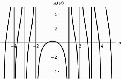
Figure 17: the function $\Lambda(p)$ as a function of real $p$.

Note that the function is symmetric about $p=1/2$. It can be readily shown that the function $\Lambda(p)$ is real if $p=-1/2\pm ik$, with $k$ real. The proper eigenfunctions and eigenvalues are associated with just such values of $p$. In fact, we can choose for eigenfunctions of the operator

$$\xi_{k}(s)=s^{-1/2}\sin\left(k\ln\frac{s}{b}+\phi(k)\right).$$ (33)

If we then require that the derivative of the eigenfunction $\xi_{k}(s)$ is zero at the boundary ($s=b$), then $\phi(k)=\arctan 2k$. It can be shown that the integrations leading to the eigenvalue are all convergent, and the eigenvalue has the form $\Lambda(-1/2+ik)$. A plot of this eigenvalue as a function of the parameter $k$ is displayed in Figure 18.

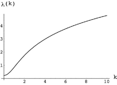
Figure 18: The function $\lambda(k)=\Lambda(-1/2+ik)$, for $k>0$.

This eigenvalue is an even function of $k$. As it turns out, an excellent numerical approximation to

$$\lambda(k)=\Lambda(-1/2+ik),$$ (34)

is given by

$$\lambda(k)\approx 0.2274112+\ln\left[1+0.929k^{2}\right]$$ (35)

The spacing of the eigenvalues is determined by the allowed values of the parameter $k$ in (34). If we assume that the eigenfunctions pass through zero at some large value of $s$, or that they have a zero slope there, then it is straightforward to show that the lowest eigenvalues will be associated with equally-spaced $k$’s. Figure 3 contains a comparison between the eigenvalues given by Eq. (34) with equally-spaced $k$’s and the numerically calculated eigenvalues of the interaction operator with matrix elements in the cosine basis set as shown in Eq. (6).

As an additional check on the validity of the results presented here, we compare the eigenfunctions in Eq. (33) to the eigenvectors of matrix in Eq. (6). The eigenvectors are plotted in real space. We find that for low eigenvalues, the expressions in Eq. (33) provide an excellent match to the results of numerical calculations. Figure 4 displays a comparison between an eigenfunction as given by Eq. (33) and the numerically-determined eigenvector associated with the sixth-lowest eigenvalue of the discrete version of the kernel. The value of $k$ in the formula for the eigenfunction was adjusted with the use of a least-squares procedure. The eigenfunctions have zero slope at the boundary of the region associated with the smallest value of $s$. The quantity $s$ does not range over the entire interval, from 0 to 1, because the analytic eigenfunctions generated here are expected to be accurate only in the regime $s\ll L$, where $L$ has been set equal to one in the case at hand.

The least-squares fitting of the analytical eigenfunctions to numerical eigenvectors leads to a set of values for the parameter, $k$. Figure 19 displays the values of $k$, plotted against the index of the eigenvalues. As indicated by the straight line drawn through them, the $k$’s are approximately equally-spaced.

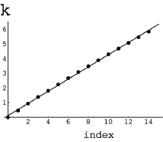
Figure 19: The values of the parameter $k$.

References

- Alberts (2002) B. Alberts, Molecular biology of the cell (Garland Science, New York, 2002), 4th ed.
- Eichinger et al. (1996) L. Eichinger, B. Koppel, A. A. Noegel, M. Schleicher, M. Schliwa, K. Weijer, W. Witke, and P. A. Janmey, Biophys J 70, 1054 (1996).
- Janmey (1999) P. A. Janmey, Current Opinion in Cell Biology 2, 4 (1999).
- Helfer et al. (2000) E. Helfer, S. Harlepp, L. Bourdieu, J. Robert, F. C. MacKintosh, and D. Chatenay, Physical Review Letters 85, 457 (2000), article Aps Access restricted.
- Kratky and Porod (1949) O. Kratky and G. Porod, Recl. Trav. Chim. 68, 1106 (1949).
- Odijk (1977) T. Odijk, J. Polym. Sci. 15, 477 (1977).
- Skolnick and Fixman (1977) J. Skolnick and M. Fixman, Macromolecules 10, 944 (1977).
- Barrat and Joanny (1993) J. L. Barrat and J. F. Joanny, Europhysics Letters 24, 333 (1993), article.
- Ha and Thirumalai (1999) B. Y. Ha and D. Thirumalai, European Physical Journal B 110, 7533 (1999).
- Golestanian et al. (1999) R. Golestanian, M. Kardar, and T. B. Liverpool, Physical Review Letters 82, 4456 (1999).
- Gennes (1979) P. G. d. Gennes, Scaling concepts in polymer physics (Cornell University Press, Ithaca, N.Y., 1979).
- Wilhelm and Frey (1996) J. Wilhelm and E. Frey, Physical Review Letters 77, 2581 (1996).
- (13) L. Le Goff, unpublished.
- Odijk (1995) T. Odijk, Macromolecules 28, 7016 (1995).
- (15) Numerical evaluation of for neutral semiflexible chains based on a Monte-Carlo simulation in Ref. Wilhelm and Frey (1996) reveals that the approximation taken for analytical calculation of is good when . Thus we restrict our attention to this regime and assume that is the onset of rodlike limit, where is an extracted effective persistence length for the case of charged chains.
- Khokhlov (1980) A. R. Khokhlov, Journal of Physics A (Mathematical and General) 13, 979 (1980).
- Zandi et al. (a) R. Zandi, J. Rudnick, and R. Golestanian, submitted to Phys. Rev. E, eprint cond-mat/0208178.
- Khokhlov and Khachaturian (1982) A. R. Khokhlov and K. A. Khachaturian, Polymer 23, 1742 (1982).
- (19) R. Netz, unpublished.
- (20) We are grateful to Dr. Itamar Borukhov for suggesting key elements of this approach.
- Zandi et al. (b) R. Zandi, J. Rudnick, and R. Golestanian, unpublished.
- Stevens and Kremer (1995) M. J. Stevens and K. Kremer, Journal of Chemical Physics 103, 1669 (1995).
- Rouzina and Bloomfield (1998) I. Rouzina and V. A. Bloomfield, Biophys. J. 74, 3152 (1998).
- Diamant and Andelman (2000) H. Diamant and D. Andelman, Physical Review E (Statistical Physics, Plasmas, Fluids, and Related Interdisciplinary Topics) 61, 6740 (2000).