Fracture of Notched Single Crystal Silicon

Abstract

We study atomistically the fracture of single crystal silicon at atomically sharp notches with opening angles of 0 degrees (a crack), 70.53 degrees, 90 degrees and 125.3 degrees. Such notches occur in silicon that has been formed by etching into microelectromechanical structures and tend to be the initiation sites for failure by fracture of these structures. Analogous to the stress intensity factor of traditional linear elastic fracture mechanics which characterizes the stress state in the limiting case of a crack, there exists a similar parameter $K$ for the case of the notch. In the case of silicon, a brittle material, this characterization appears to be particularly valid. We use three interatomic potentials: a modified Stillinger-Weber potential, the Environment-Dependent Interatomic Potential (EDIP), and the modified embedded atom method (MEAM). Of these, MEAM gives critical $K$-values closest to experiment. In particular the EDIP potential leads to unphysical ductile failure in most geometries. Because the units of $K$ depend on the notch angle, the shape of the $K$ versus angle plot depends on the units used. In particular when an atomic length unit is used the plot is almost flat, showing—in principle from macroscopic observations alone—the association of an atomic length scale to the fracture process.

I Introduction

Recently there has been experimentalDunn et al. (1997); Suwito et al. (1998, 1999) and theoreticalZhang (2002) interest in fracture in sharply notched single crystal silicon samples. Such samples have technological importance because silicon is a commonly used material in the fabrication of MEMS devices; the etching process used tends to create atomically sharp corners due to highly anisotropic etching rates.Suwito et al. (1999) Failure in such devices is often a result of fracture which initiated at sharp corners.Suwito et al. (1997) In the case of a notch, there exists a parameter $K$ analogous to the stress intensity factor of traditional fracture mechanics, which parameterizes the elastic fields in the vicinity of the notch. Suwito et al.Suwito et al. (1998, 1999) have carried out a series of experiments which have (i) established the validity of the stress intensity factor as a fracture criterion in notched specimens and (ii) measured the critical stress intensities for several notch geometries. On the theoretical side ZhangZhang (2002) has carried out an analysis which models the separation of cleavage planes by a simple cohesive law, and thereby derived a formula for the critical stress intensity as a function of notch opening angle. The material properties which enter this formula are the elastic constants and the parameters of the cohesive law, the peak stress $\hat{\sigma}$ and the work of separation $\Gamma_{0}$. This recent activity has prompted us to investigate the phenomenon of fracture in notched silicon using atomistic simulations: In this paper we present direct measurements of the critical stress intensity for different geometries (i.e., notch opening angles) and compare them to the experimental results of Suwito et al. We apply a load by specifying a pure $K$-field of a given strength (stress intensity factor) on the boundary of the system. In doing this we are effectively using the result of Suwito et al. that the notch stress intensity factor is indeed the quantity which determines fracture initiation, so we can ignore higher order terms in the local stress field.

I.1 Elastic fields near a notch

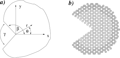
Figure 1: (a) Notch schematic and notation; (b) silicon crystal with a notch; darker layer is fixed boundary atoms.

The essential geometry of a notch is shown in Fig. 1. The notch opening angle is denoted $\gamma$ and the half-angle within the material, which is the polar angle describing the top flank, is $\beta$ (thus $\beta=\pi-\gamma/2$). As discussed in detail by Suwito et al.,Suwito et al. (1998, 1999) it is fairly straightforward to solve the equations of anisotropic linear elasticity for a notched specimen. The formalism used is known as the Stroh formalism,Ting (1996) which is useful for dealing with materials with arbitrary anisotropy in arbitrary orientations, as long as none of the fields depend on the $z$ coordinate (this will be the out-of-plane coordinate; note that this does not restrict the deformation itself to be in-plane). Here we only consider mode I (symmetric) loading. The displacement and stress fields for a notch can be written as

$$u_{i}=Kr^{\lambda}g_{i}(\theta)$$ (1)

$$\sigma_{ij}=Kr^{\lambda-1}f_{ij}(\theta)$$ (2)

where $\lambda$ plays a role like an eigenvalue; its value is determined by applying the traction-free boundary conditions to the notch flanks. There is an infinity of possible values for $\lambda$ of which we are interested in those in the range $0<\lambda<1$, which give rise to a singular stress field, often known as the $K$-field, at the notch tip. This is entirely analogous to the singular field near a crack tip, which is simply the limiting case where $\gamma$ goes to zero ($\beta\longrightarrow\pi$), and $\lambda$ becomes one half. Further details of the Stroh formalism, as applied to the notch geometry, are given in appendix B. The complete elastic solution involves the whole infinity of values for $\lambda$, corresponding to different multipoles of the elastic field. Negative values of $\lambda$ correspond to more singular fields which are associated with properties of the core region stemming from the non-linear atomistic nature of this region; they do not couple to the far-field loading. $\lambda>1$ corresponds to fields which are less singular, and do not influence conditions near the notch-tip, since the displacements and stress vanish there. They are, however, essential to represent the full elastic field throughout the body, and ensure that boundary loads and displacements (whatever they may be) are correctly taken into account. This is the basis for asserting that only the $K$-field is important. This field is unique among the multipoles in that it both couples to the far-field loading and is singular at the notch tip. Thus the stress intensity factor must characterize conditions at the crack tip, and therefore a critical value, $K_{c}$, is associated with the initiation of fracture. The validity of this approach hinges on the validity of linear elasticity to well within the region in which the $K$-field dominates.

Figure 2: Normal (a) and shear (b) stresses on radial planes as functions of plane angle, for $\gamma=70^{\circ}$.

From Eq. (2) we see that the units of $K$ and therefore $K_{c}$ are $stress/length^{\lambda-1}$ which depends continuously on the notch angle $\gamma$ through $\lambda$. Hence the shape of a plot of $K_{c}$ against notch angle depends on the units used to make the plot. In metric/SI units $K_{c}$ changes by an order of magnitude between $70^{\circ}$ and $125^{\circ}$ whereas if an atomic scale unit of length is used the plot is nearly flat (Fig. 15). The most interesting feature of this is that it seems to provide a direct link from macroscopic measurements to a microscopic length scale. From a continuum point of view, one incorporates atomistic effects into fracture via a cohesive zone, a region ahead of the crack tip where material cleaves according to a specified force-separation law. One of the parameters of such laws is the length scale—the distance two surfaces must separate before the attractive force goes to zero—which for a brittle material is an atomic length scale. It is this scale that one would identify from the plot of $K_{c}$ versus angle. Note that one can only identify a scale, and not an actual length parameter, in particular because the different geometries that are involved in the plot involve different fracture surfaces, with presumably different force-separation parameters.

Table 1: Surface energies for silicon according to mSW, EDIP and MEAM potentials.

potential	surface	atomic units	SI units
mSW	111	0.0906	1.3593
mSW	110	0.1110	1.6649
mSW	100	0.1570	2.3545
EDIP	111	0.06538	1.0475
EDIP	110	0.08194	1.3128
EDIP	100	0.1320	2.1150
MEAM	111	0.07668	1.2285
MEAM	110	0.09030	1.4469
MEAM	100	0.08126	1.3019

Fig. 2 shows the normal and shear stresses on radial planes (perpendicular to the plane of the sample) emanating from the notch tip, for unit $K$ and $r$ (i.e., they are derived from the tensor $f_{ij}$ appearing in Eq. (2)). The figures show the functions for the $\gamma=70^{\circ}$ case; the other geometries have the same qualitative behavior. Both stresses vanish at the maximum angles, corresponding to the notch flanks; this is in accordance with traction-free boundary conditions. What is most important to note is that the normal stress, which presumably is most relevant for cleavage on a radial plane, has its maximum at $\theta=0$. The shear stress, which is relevant for possible slip behavior (dislocations) which could compete with cleavage as a means of relieving stress, is zero at $\theta=0$, and has a maximum at intermediate angles. If there is an easy crystal slip plane in the vicinity of the maximum, slip could conceivably compete with cleavage.

II Simulation

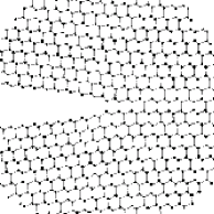
(a) $K=0.3064$

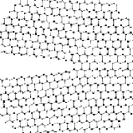
(b) $K=0.3068$

Figure 3: mSW-crack.

II.1 Geometry

We simulated a cylindrical piece of silicon with a notch, making a ‘PacMan’ shape as in Fig. 1(b), consisting of an inner core region and an outer boundary region. By focusing on just the initiation of fracture we avoid the need for large systems since we are not interested in the path the crack takes after the fracture (if we were, we would have a problem when the crack reached the edge of the core region and hit the boundary which is only a few lattice spacings away). We consider three notch geometries, which we call the $70^{\circ}$ (actually $70.5288^{\circ}$), $90^{\circ}$ and $125^{\circ}$ (actually $125.264^{\circ}$) geometries respectively, referring to the notch opening angles. The $70^{\circ}$ sample has {111} surfaces on the notch flanks and the plane of the sample is a {110} surface. The $90^{\circ}$ sample has {110} surfaces on the flanks and the plane is a {100} surface (in this case the crystal axes coincide with the coordinate axes). The $125^{\circ}$ sample has a {111} on the bottom flank and a {100} surface on the top flank, while the plane of the sample is a {110} plane. In addition, we studied the zero degree notch geometry, corresponding to a standard crack. The crack plane is a {111} surface and is the $xz$ plane in the simulation, and the direction of growth is the $\langle 211\rangle$ direction, which is the $x$ direction in the simulation. The radius of the inner, core region in almost all the cases presented is 5 lattice spacings or about 27 Å. The exceptions were the crack geometry for the EDIP potential (core radius was 7.5 lattice spacings—the larger size makes the ductile behavior of the potential more obvious) and the $90^{\circ}$ geometry with the MEAM potential (core radius was four lattice spacings because this potential is computationally more demanding). The coordinate system in each case is oriented so that the plane of the sample is the $xy$ plane and the notch is bisected by the $xz$ plane.

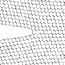
(a) $K=0.3$

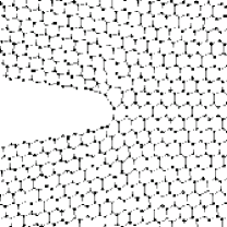
(b) $K=0.4$

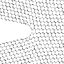
(c) $K=0.56$

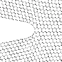
(d) $K=0.6$

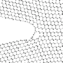
(e) $K=0.66$

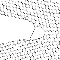
(f) $K=0.76$

Figure 4: EDIP-crack.

II.2 Potentials

We have used three different silicon potentials. The first is a modified form of the Stillinger-Weber Stillinger and Weber (1985) potential (mSW), in which the coefficient of the three body term has been multiplied by a factor of 2. This has been noted by Hauch et al.Hauch et al. (1999) to make the SW potential brittle; they were unable to obtain brittle fracture with the unmodified SW potential. However it worsens the likeness to real silicon in other respects such as melting point and elastic constants.Holland and Marder (1998, 1999); Hauch et al. (1999) The second potential is a more recent silicon potential known as “environment-dependent interatomic potential” (EDIP),Bazant et al. (1997); Justo et al. (1998) which is similar in form to SW but has an environmental dependence that makes it a many-body potential. Bernstein and coworkersBernstein et al. (1999); Abraham et al. (2000); Bernstein and Hess (2001) have used EDIP to simulate fracture in silicon. They reported a fracture toughness about a factor of four too large when compared with experiment, and that fracture proceeds in a very ductile manner, accompanied by significant plastic deformation and disorder. On the other hand, using tight-binding molecular dynamics near the crack tip they successfully simulated brittle fracture in silicon. In view of the failure of many empirical potentials to simulate brittle fracture, Pérez and GumbschPérez and Gumbsch (2000) used density functional theory to simulate the fracture process, measuring lattice trapping barriers for different directions of crack growth on different fracture planes. A reason for the failure of empirical potentials that has been proposed in Ref. Bernstein and Hess, 2001 is that their short-ranged nature necessarily requires large stresses to separate bonds. This however is not the case in our third potential, which is the modified embedded atom method (MEAM) of Baskes.Baskes (1992) This is a many-body potential similar to the embedded atom method but with angular terms in the electron density; it has been fit to many elements including metals and semi-conductors. A significant feature of this potential is its use of “three-body screening” in addition to the usual pair cut-off distance. This means that atoms in the bulk see only their nearest neighbors, while surface atoms, on the other hand, can see any atoms above the surface (for example on the other side of a crack) within the pair cut-off distance. The pair cut-off has been set to 6 Å to allow the crack surfaces to see each otherBaskes (2002) even after they have separated. The MEAM potential has been used successfully to simulate dynamic fracture in silicon,Baskes (2002) and we have found it to be the most reliable potential in our studies of notch fracture. In table 1 we list the low-index (relaxed, unreconstructed) surface energies for the three potentials.

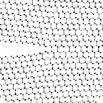
(a) $K=0.183$

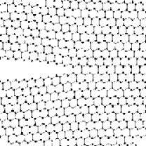
(b) $K=0.1835$

Figure 5: MEAM-crack.

II.3 Boundary Conditions

The boundary conditions are as follows: in the $z$-direction (out of the page) there are periodic boundary conditions. The thickness of the sample in this direction is always one or two repeat distances of the lattice in that direction. For the $70^{\circ}$ and $125^{\circ}$ geometries the repeat distance is $\sqrt{2}a$ where $a$ is the cubic lattice constant; for the $90^{\circ}$ geometry it is $2a$. In the plane, the boundary conditions are that an layer of atoms on the outside of the system has the positions given by the analytic formula (1) for displacements from anisotropic linear elasticity, with a specified stress intensity factor $K$. The thickness of the layer is twice the cutoff distance of the potential, in order that the core atoms feel properly surrounded by material. We interpret the displacement formulas in terms of Eulerian coordinates, using an iterative procedure to compute the current positions. The numbers of core atoms were 890, 894, 1260, and 892, for the $0^{\circ}$ (crack), $70^{\circ}$, $90^{\circ}$ and $125^{\circ}$ systems respectively (except for the EDIP/crack case where the core radius was 7.5 lattice constants; there the number of core atoms was 2002). The number of boundary atoms depends on the potential (through the cutoff distance); it is typically about 500 atoms. For the most part no special consideration was given to the lattice origin, which meant that by default it coincided with the notch tip. In a few cases it was necessary to shift the position of the origin in order to make sure that the notch flanks were made cleanly, in particular so that the {111} flanks in the $70^{\circ}$ and $125^{\circ}$ geometries were complete close packed {111} surfaces, rather than having dangling atoms.

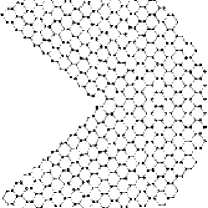
(a) $K=0.3828$

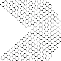
(b) $K=0.3832$

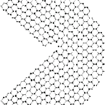
(c) $K=0.4306$

Figure 6: mSW-$70^{\circ}$.

II.4 Critical stress intensities

The simulation consists of alternating the following two steps: (1) We increment the value of $K$ by a small amount, changing the positions of the boundary atoms accordingly. (2) We relax the interior atoms as follows. First we run about 50 steps of Langevin molecular dynamics with a temperature of 500–600 K; the purpose of this is to break any symmetry (the $70^{\circ}$ and $90^{\circ}$ samples are symmetric about the $xz$ plane). It is still a zero temperature simulation; these finite temperature steps are simply a way to introduce some noise. Next we run 500 time steps of the dynamical minimization technique known as “MDmin” (a Verlet time step is carried out, but after each velocity update, atoms whose velocities have negative dot-products with their forces have their velocities set to zero). Finally 500 time steps of conjugate gradients minimization are carried out. We observe that the combination of both types of minimization is more effective (converges to a zero force state more quickly) than either alone. The procedure generally results in the atoms having forces of around $10^{-5}eV/$Å.

The initial value for $K$ could be zero; however it turns out to be possible to start from a fairly large value of $K$ by applying the analytic displacements to the whole system at first. When the critical $K$ value, $K_{c}$, is not yet known the increment size is chosen reasonably large to quickly find the $K_{c}$. When this has been found, the simulation is restarted from a value below the critical value with smaller increments and a more accurate value for $K_{c}$ found. The increment is a measure of the uncertainty in $K_{c}$.

III Results

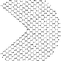
(a) $K=0.2455$

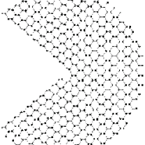
(b) $K=0.2465$

Figure 7: EDIP-$70^{\circ}$.

III.1 Observed fracture behavior

We observe brittle cleavage of the simulated crystals at definite values of $K$ for all geometries using the mSW and MEAM potentials, but only for the $70^{\circ}$ geometry when using the EDIP potential. Figures 3–14 show snapshots of the simulation process for the different geometries and potentials. In most cases two or three snapshots are shown: one of the configuration immediately before crack initiation, one of the configuration immediately after initiation, and possibly one of a “late-stage” configuration, to illustrate the fracture plane more vividly; generally this was chosen to be the configuration corresponding to the highest applied load, which depended on how long the simulation was run past the initiation point. For the EDIP potential, which gives unphysical ductile behavior (except in one case, the $70^{\circ}$ geometry), more snapshots are shown, in order to illustrate the plastic behavior more completely, since a variety of stages is involved.

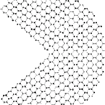
(a) $K=0.266$

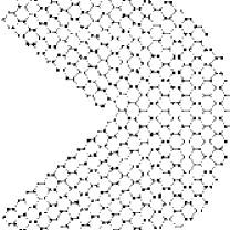
(b) $K=0.268$

Figure 8: MEAM-$70^{\circ}$.

The behavior in crack geometries is shown in Figs. 3–5. The initial applied load must be such that no crack healing takes place upon relaxation, so that the location of the crack corresponds to the center of the system (in reference to which the boundary displacements are calculated). In this case we are not investigating crack initiation (since the notch is already a crack)but crack growth; the critical $K_{c}$ is defined as that at which the crack advances, or when the next bond across the crack plane breaks. This is somewhat hard to see in the figures; one must count atoms along the crack surface and compare from one figure to another to see that growth has occurred.

(a) $K=0.3860$

(b) $K=0.3863$

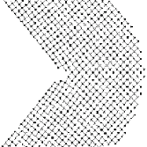
(c) $K=0.3871$

Figure 9: mSW-$90^{\circ}$.

The mSW and MEAM potentials produce similar, brittle, fracture behavior. The EDIP potential produces quite different behavior; the crack propagates in a ductile manner. Frame (a) shows the configuration before any plastic deformation has taken place. Frame (b) shows what appears to be the nucleation of a dislocation onto the {110} slip plane which is at an angle of $54.6^{\circ}$ to the positive $x$-axis. By frame (c) the crack tip has blunted noticeably, and in frame (d) a growth of the blunted crack by about a lattice constant has taken place—we take the stress intensity at this stage to be the critical value. Frames (e) and (f) show a void nucleating and growing behind the crack tip, which would under further loading join with the crack—coalescence of voids the essence of ductile crack growth.

(a) $K=0.451$

(b) $K=0.491$

(c) $K=0.511$

(d) $K=0.521$

(e) $K=0.531$

(f) $K=0.6$

Figure 10: EDIP-$90^{\circ}$.

In the $70^{\circ}$ system (Figs. 6–8) fracture occurs along a {111} plane. There are two choices for this, symmetrically placed with respect to the $xz$ plane. Here all three potentials produced brittle behavior; this was the only geometry in which the EDIP potential did so. Possible reasons for this exception are discussed in section IV. However, when the origin was not shifted as mentioned in section II.4, so that the notch flanks had dangling atoms, the EDIP-behavior was quite different: the notch blunted to a width of several atomic spacings.

(a) $K=0.293$

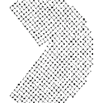
(b) $K=0.2935$

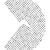
(c) $K=0.34$

Figure 11: MEAM-$90^{\circ}$.

The behavior for $90^{\circ}$ models is shown in Figs. 9–11. We observe three different behaviors for three different potentials—providing a cautionary demonstration of the limitations of empirical potentials. The easy cleavage planes available here are the {110} planes which are extensions of the notch flanks. The mSW model starts to cleave along the lower of these (the extension of the upper flank) but the crack advances only one atomic before cleavage switches to an adjacent parallel plane. The net result is a kind of “unzipping” along the hard {100} plane. This is presumably because the peak in the normal stress across this plane, compared to the normal stress at the $45^{\circ}$ angle, outweighs the increased cost of cleavage (but note that the surface energy ratio $\gamma_{100}/\gamma_{111}$ is in fact lower for MEAM, which cleaves on the {110} plane—see table 1 for the energies of the different surfaces according to the different potentials). The EDIP potential deforms plastically in this case, as depicted in the six frames of Fig. 10. It is harder to identify specific processes here than in the $70^{\circ}$ case, including where crack growth starts, though it seems to have definitely started by the frame (c)($K_{c}=0.6$). The MEAM potential behaves in the manner most consistent with experiment, namely cleaving on {110} planes, and switching from one to the other—this is illustrated dramatically in the third frame of Fig. 11. Experimentally, switching between planes, when it happens, occurs over longer length scales ($25\mu m$ for the $70^{\circ}$ caseSuwito et al. (1998)), although the behavior at atomic length scales has not been examined. Too much should not be read into the switching we observe, because once cleavage has occurred over such distances the proximity of the boundary probably has a large effect on the effective driving force on the crack.

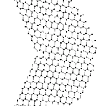
(a) $K=0.3302$

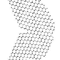
(b) $K=0.3304$

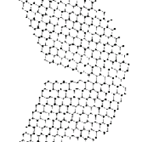
(c) $K=0.3323$

Figure 12: mSW-$125^{\circ}$.

For the $125^{\circ}$ geometry (Figs. 12–14), there are again two {111} planes to choose from but they are not symmetrically placed. Fracture occurs for the mSW and MEAM potentials on the one closest to the $xz$ plane, i.e., closest to the plane of maximum normal stress, which is the $(11\bar{1})$ plane. The direction of growth is $[21\bar{1}]$, and growth proceeds much more readily than in the other notch geometries, presumably because it is almost along the maximum stress plane. In the EDIP system, plastic deformation is favored over cleavage. This appears to proceed as follows: First, slip occurs on the $(11\bar{1})$ plane in the $[21\bar{1}]$ direction, as a single edge dislocation is nucleated (frame (a)–frame (b)). Next, slip occurs on the other {111} plane, the $(1\bar{1}1)$ plane, in the $[21\bar{1}]$ direction, with two dislocations being nucleated (frame (b)–frame (c)–frame (d)), on adjacent $(1\bar{1}1)$ planes. In the last two frames a void appears and grows.

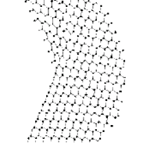
(a) $K=0.43$

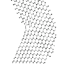
(b) $K=0.44$

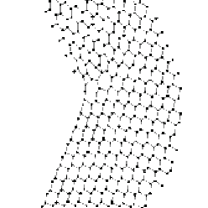
(c) $K=0.52$

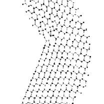
(d) $K=0.57$

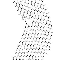
(e) $K=0.58$

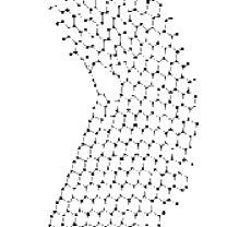
(f) $K=0.59$

Figure 13: EDIP-$125^{\circ}$.

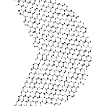
(a) $K=0.2195$

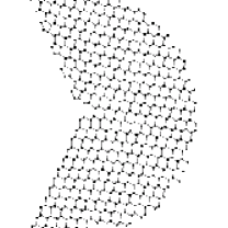
(b) $K=0.22$

Figure 14: MEAM-$125^{\circ}$.

III.2 Critical stress intensities

The values of $K_{c}$, for the different potentials as well as from experiment, are listed in table 2 and plotted in Fig. 15. The increment size for $K$ is listed as an estimate of the error in $K_{c}$. The values for ductile fracture from the EDIP potential are marked with an asterisk as a reminder that the definition of $K_{c}$ in these cases is problematic. The experimental value for the crack geometry is from Ref. Chen and Leipold, 1980. Notice that the critical stress intensities for difference angles are almost the same in atomic units, and differ by more than a factor of ten in standard units To check for finite size effects, we repeated the measurement on the $70^{\circ}$ geometry, but with larger radius of 8 Å, using the MEAM potential. In this case $K_{c}$ was determined to be $0.262\pm 0.001$, or about $1.7$% lower than the value from the smaller system. This indicates that finite size effects are small, but not negligible. To compensate for them without using larger systems a flexible boundary method could be used, involving higher order “multipoles” of the elastic field, appropriate for the notch (i.e., solutions with $\lambda<0$), which could be relaxed.

Table 2: Critical stress intensity values for different geometries and potentials, including experimental data from Refs. Suwito et al., 1998, 1999.

Potential	Geom.	$K_{c}$	Error	Griffith	$K_{c}$ (SI)
mSW	0	0.3068	0.00036	0.19509	$4.9\times 10^{5}$
mSW	70	0.3832	0.00036	-	$9.6\times 10^{5}$
mSW	90	0.3863	0.00035	-	$1.78\times 10^{6}$
mSW	125	0.3304	0.00016	-	$1.07\times 10^{7}$
EDIP	0	0.6*	0.02	0.14634	$9.6\times 10^{5}$
EDIP	70	0.2465	0.001	-	$6.1\times 10^{5}$
EDIP	90	0.5–0.6*	0.0005	-	$2.4$–$2.8\times 10^{6}$
EDIP	125	0.5–0.6*	0.001	-	$1.5$–$1.8\times 10^{7}$
MEAM	0	0.184	0.0005	0.16406	$3\times 10^{5}$
MEAM	70	0.2665	0.0005	-	$6.57\times 10^{5}$
MEAM	90	0.2935	0.0005	-	$1.42\times 10^{6}$
MEAM	125	0.22	0.0005	-	$6.47\times 10^{6}$
Expt	0	0.2060	-	0.1776	$3.3\times 10^{5}$
Expt	70	0.31	10%	-	$7.6\times 10^{5}$
Expt	90	0.43	10%	-	$2.1\times 10^{6}$
Expt	125	0.22	10%	-	$6.5\times 10^{6}$

IV Discussion

IV.1 Critical stress intensities

Comparisons are easier to make when looking at the data plotted using atomic scale units. Then the data for the two brittle potentials is a gentle, almost horizontal, curve. The experimental data mostly lies between that for the MEAM potential and that for the mSW potential, but significantly closer to the former. The exception is the $90^{\circ}$ case where the experimental value jumps to higher than the mSW value. Since the curves from the two potentials are very similar in shape—the main difference seems to be an overall shift or factor—and the jump in the experimental value at $90^{\circ}$ is a departure from this shape, it would not be meaningful to assert that the mSW potential does a better job in predicting $K_{c}$ in the $90^{\circ}$ case. For the other angles the MEAM values are more or less within experimental error of experiment: the error (standard deviation across all the tested samples) is close to 10% in all cases (the error is not available for the crack case), and the percentage differences of the MEAM values with respect to the experimental values are $-10$%, $-14$%, $-32$% and $-0.5$% for the $0^{\circ}$, $70^{\circ}$, $90^{\circ}$ and $125^{\circ}$ geometries respectively. The 0.5% is clearly fortuitous. Note that the experimental error bar is not enough to account for the anomalously high value for the $90^{\circ}$ case; there must be some feature of the physics or energetics of fracture initiation in this geometry that is missing from the others, and missing from the simulation.

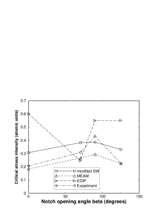
(a) Units based on $eV$ and Å 

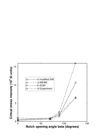
(b) SI units

Figure 15: Computed critical stress intensities for the three potentials and experiment.

An interesting question is why the EDIP potential behaves unlike the other potentials and experiment except at one particular geometry, the $70^{\circ}$ one. Possibly there is some feature of this geometry that suppresses the nucleation of dislocations. Dislocation Burgers vectors in silicon are always in $\mbox{$\frac{1}{2}$}\langle 110\rangle$ directions, since these are the shortest perfect lattice vectors in the diamond lattice.Hirth and Lothe (1982) The periodic boundary conditions constrain possible dislocation lines to be out of the plane. Moreover, since we are considering only mode I and II loading, we expect slip to be within the plane, so we consider only edge dislocations. In the $70^{\circ}$ geometry the $\mbox{$\frac{1}{2}$}\langle 110\rangle$ direction that is available within the plane is at an angle of $90^{\circ}$ to the $x$-axis, while the cleavage plane is at an angle of $35.26^{\circ}$. Looking at Fig. 2, we can see that the shear stress and normal stresses on these planes respectively are both near their maximum values, although the ratio of shear stress to normal stress is 0.43 (both plots are normalized with respect to $K$ and $r$.). Without knowing the values of stress needed to initiate slip or cleavage on these respective planes, this ratio is not enough to explain anything. What we can do is compare the same ratio for the other geometries and check if it is higher in other cases, thereby tending to make slip more favorable than cleavage, for a given potential (namely, EDIP). The numbers—angles for slip and cleavage and the appropriate stress ratio—are shown in table 3. Unfortunately, there is no conclusive trend. The ratio for $90^{\circ}$ is indeed higher than that for $70^{\circ}$ but the others are lower, and EDIP notches suffer plastic deformation in all of the other cases.

Table 3: Angles of slip planes and crack planes and ratio of shear to normal stress for different geometries.

geometry	slip plane	crack plane	shear/normal
70	$90^{\circ}$	$35.26^{\circ}$	0.43
90	$45^{\circ}$	$45^{\circ}$	0.52
125	$27.34^{\circ}$	$-7.90^{\circ}$	0.34
0	$54.6^{\circ}$	$0^{\circ}$	0.37

For the crack cases we can make a comparison of our results with the so-called Griffith criterion for crack propagation. This comes from setting the energy release rate equal to twice the surface energy. An expression for the mode I energy release rate in terms of the stress intensity factor is given in Ref. Sih et al., 1965; setting it equal to twice the surface energy leads to the following expression for the critical stress intensity factor

$$\mathbf{K}_{\text{Griffith}}=\left(\frac{2\gamma}{\pi b_{22}\text{Im}((\mu_{1}+\mu_{2})/(\mu_{1}\mu_{2}))}\right)^{\mbox{$\frac{1}{2}$}}$$ (3)

where $\mu_{1}$ and $\mu_{2}$ are the roots of a characteristic polynomial which depends on the elastic constants and $b_{22}$ is an element of the compliance tensor for plane strain. The ratio $K_{c}/K_{\text{Griffith}}$ is associated with lattice trapping, when fracture is brittle. This ratio is 1.57 for the mSW potential and 1.12 for MEAM. These values are respectively somewhat larger and somewhat smaller than the ratio 1.25 determined by Pérez and Gumbsch using total energy pseudopotential calculationsPérez and Gumbsch (2000) (our $K_{c}$ corresponds to their $K_{+}$). In the EDIP case, where fracture proceeds only accompanied by significant plastic deformation, $K_{c}$ is four times the Griffith value.

In our simulations, for a given potential, only one fracture behavior is observed, in contrast to what was observed in the experiments of Suwito et al.Suwito et al. (1998) Specifically, in the case of the $70^{\circ}$ geometry, they observed three different “modes” (not to be confused with loading modes), including propagation on the (110) plane, yet we have observed cleavage only on {111} planes in this geometry. It is possible that finite temperature, and the relative heights of different lattice trapping barriers, play an important role here. More likely it is related to experimental microcracks or defects near the crack tip. In any case, it would be of great benefit to systematically calculate the barriers for different processes that can occur at a notch (or crack) tip, as a function of applied load.

A further point to note, and a warning, is this: In comparing simulations involving such very small length scales (27 Å) to experiment it is appropriate to consider the question of whether the experimental notches are indeed as sharp as we have made our simulated notches. Suwito et al.Suwito et al. (1998) could only put an upper limit of $0.8\mu m$ on the radius of curvature of their notches, although notch radii of the order of $10nm$ have been reported in etched silicon. The addition of just a few atoms right at the notch tip would presumably have a significant effect on the energetics of cleavage initiation. We have not made any investigation of this, and this question should be borne in mind given the absence of experimental data characterizing the notch tip at the atomic scale. Nevertheless, the success of our simulations provides an important indication that these notches are indeed atomistically sharp.

V Summary

We have determined by atomistic simulation the critical stress intensities to initiate fracture in notched single crystal silicon samples. The samples had angles of $0^{\circ}$ (a crack), $70.5233^{\circ}$, $90^{\circ}$ and $125.264^{\circ}$—chosen so that the flanks of the notches were low index crystal planes. These geometries correspond to those studied experimentally in measurements of critical stress intensities for fracture initiation. Of the three potentials used, modified Stillinger-Weber (mSW), environment-dependent interatomic potential (EDIP) and modified embedded atom method (MEAM), MEAM produced the most realistic behavior. The mSW potential produced brittle fracture, but its resemblance to silicon in other respects is quite weak. Except in the case of the $70^{\circ}$ notch, the EDIP potential gives ductile fracture with a critical stress intensity factor, which is much higher than that determined using the other potentials, or by experiment.

VI Acknowledgments

We thank Zhiliang Zhang for inspiration and helpful discussions, and Noam Bernstein for helpful discussions. We also thank Mike Baskes for help in coding the MEAM potential. This work was financed by NSF-KDI grant No. 9873214 and NSF-ITR grant No. ACI-0085969. Atomic position visualization figures were produced using the dan program, developed by N. Bernstein at Harvard University and the Naval Research Laboratory.

Appendix A Units and Conversions

Three different sets of units are used in this paper. To each atomic potential (Stillinger-Weber, EDIP, MEAM) is associated a set of atomic units (EDIP and MEAM use the same units); also we often wish to use SI units to compare to experiment. In the context of this paper there is the further subtlety that the units of the chief quantity under consideration, namely the stress intensity factor $K$, are not simple powers of base units but involve a non-trivial exponent $\lambda$ which is a function of geometry and potential. In fact the SI units units for $K$ are $Pa\,m^{1-\lambda}$ which for brevity we simply refer to as ‘standard units’ in the paper.

The units for an atomic potential are determined by specifying the unit of energy and that of length (for dynamics the unit of time is determined from these and the particle mass). The SW potential as originally written down did not have units built into it. By taking the energy unit to be $\epsilon=2.1672eV=3.4723\times 10^{-19}J$ and the length unit to be $\sigma=2.0951$ Å, the authors modeled molten silicon.Stillinger and Weber (1985) However other authorsBalamane et al. (1992) have taken the energy unit to be $\epsilon=2.315eV$. The difference is not really important since we have modified the potential itself to make it more brittle so the resemblance to real silicon is reduced noticeably. When expressing quantities in terms of $eV-$Åunits we use the second scaling which is more common. The EDIP and MEAM potentials have $\epsilon=1eV$ and $\sigma=1$Åbuilt in as their units. Since $\sigma\sim Kr^{\lambda-1}$, the units of $K$ are $[stress]/[length]^{\lambda-1}=[energy]/[length]^{2+\lambda}$, so to convert a value for $K$ in atomic units to SI units, one uses the conversion factor $\epsilon/\sigma^{2+\lambda}$. Table 4 gives the factors for the three potentials and the geometries studied in this paper.

Table 4: Unit conversion factors for $K$.

Potential	geometry	$\lambda$	factor
mSW	0	0.5	1602000
mSW	70	0.51954	2510000
mSW	90	0.54597	4620000
mSW	125	0.63047	32320000
EDIP	0	0.5	1602000
EDIP	70	0.51922	2490000
EDIP	90	0.54708	4730000
EDIP	125	0.62844	30840000
MEAM	0	0.5	1602000
MEAM	70	0.51875	2467000
MEAM	90	0.54794	4832000
MEAM	125	0.62639	29420000

Appendix B Stroh formalism for notches

Here we summarize the application of the Stroh formalism to the notch problem. More details are available in Refs. Suwito et al., 1998, 1999; Labossiere and Dunn, 1998. We can write the solution for the displacement field $\mathbf{u}$ and the stress function $\phi$ as

$$\mathbf{u}=\sum_{\alpha=1}^{6}\mathbf{a}_{\alpha}f_{\alpha}(z_{\alpha})$$ (4)

$$\phi=\sum_{\alpha=1}^{6}\mathbf{b}_{\alpha}f_{\alpha}(z_{\alpha})$$ (5)

The independent variable here is the complex variable $z_{\alpha}=x_{1}+p_{\alpha}x_{2}$. The stress function $\phi$ determines the stresses through $\sigma_{i1}=-\phi_{i,2}$ and $\sigma_{i2}=\phi_{i,1}$. The $p_{\alpha},\mathbf{a}_{\alpha}$ and $\mathbf{b}_{\alpha}$ come from solving the following eigenvalue problem:

$$(\mathbf{Q}+p(\mathbf{R+R^{T}})+p^{2}\mathbf{T})\mathbf{a}=0$$ (6)

where

$$\begin{split}\mathbf{Q}&=\left[\begin{array}[]{ccc}C_{11}&C_{16}&C_{15}\\ C_{16}&C_{66}&C_{56}\\ C_{15}&C_{56}&C_{55}\end{array}\right]\mathbf{R}=\left[\begin{array}[]{ccc}C_{16}&C_{12}&C_{14}\\ C_{66}&C_{26}&C_{46}\\ C_{56}&C_{25}&C_{45}\end{array}\right]\\ \mathbf{T}&=\left[\begin{array}[]{ccc}C_{66}&C_{26}&C_{46}\\ C_{26}&C_{22}&C_{24}\\ C_{46}&C_{24}&C_{44}\end{array}\right]\end{split}$$ (7)

The above is general within the context of two-dimensional anisotropic elasticity. To specify the notch problem we choose a form of the arbitrary function $f$ to which we can apply the boundary conditions of the problem—that notch flanks are traction-free. The following choice does the trick:

$$f_{\alpha}(z_{\alpha})=\frac{1}{\lambda}\frac{z_{\alpha}^{\lambda}}{\xi_{\alpha}(-\beta)^{\lambda}}\mathbf{b^{T}}_{\alpha}\mathbf{q}=\frac{1}{\lambda}r^{\lambda}\left[\frac{\xi_{\alpha}(\theta)}{\xi_{\alpha}(-\beta)}\right]^{\lambda}\mathbf{b^{T}}_{\alpha}\mathbf{q}$$ (8)

where $\xi(\theta)=\cos(\theta)+p_{\alpha}\sin(\theta)$ and $\mathbf{q}$ is to be determined. The traction with respect to a radial plane at angle $\theta$ is given by

$$\mathbf{t}=r^{\lambda-1}\sum_{\alpha=1}^{6}\left[\frac{\xi_{\alpha}(\theta)}{\xi_{\alpha}(-\beta)}\right]^{\lambda}\mathbf{b}_{\alpha}\mathbf{b^{T}}_{\alpha}\mathbf{q}=\frac{\lambda}{r}\phi$$ (9)

With the above form the traction condition is already satisfied on the bottom flank $\theta=-\beta$. Applying the condition on the top flank leads to a matrix equation

$$\mathbf{K}(\lambda)\mathbf{q}(\lambda)=0$$ (10)

The appropriate value of $\lambda$ is determined by setting the determinant of the matrix equal to zero and solving the resulting equation numerically. In the range $0<\lambda<1$, two values can be found, corresponding to modes I and II, $\lambda^{I}$ and $\lambda^{II}$. For a given $\lambda$, the vector $\mathbf{q}$ is determined up to a normalization which is related to how one defines the stress intensity factor $K$. Thus we obtain expressions for the displacements which are used in the simulation to place the boundary atoms. In the crack case, because $\lambda^{I}$ and $\lambda^{II}$ are degenerate at the value $1/2$, the definition of modes I and II is a little subtle. The {111} plane is not a plane of symmetry of the cube, and thus one cannot expect to separate modes by their symmetry properties as in for example, the isotropic case; following Ref. Sih et al., 1965, mode I is defined as that for which $\sigma_{12}(\theta=0)=0$ and mode II that for which $\sigma_{22}(\theta=0)=0$.

For the purpose of the simulations described in this paper, we calculated the Stroh parameters as follows. For each potential, the elastic constants were determined by standard methods (straining the supercell, relaxing, measuring the relaxed energy per unit undeformed volume and fitting to a parabola). This gives $C_{11}$, $C_{12}$, and $C_{44}$, which are the three independent constants for a cubic crystal. In the formulas for the displacements and stresses given above, the coordinate system is aligned with the notch (in that the negative $x$-axis bisects the notch itself) and not with the crystal axes. So we must transform the elastic constants accordingly. Once we have the transformed constants we can construct the Stroh matrices ${\mathbf{Q}}$, ${\mathbf{R}}$ and ${\mathbf{T}}$, and compute the Stroh eigenvalues and eigenvectors as above.

References

- Dunn et al. (1997) M. L. Dunn, W. Suwito, S. J. Cunningham, and C. W. May, Int. J. Fract. 84, 367 (1997).
- Suwito et al. (1998) W. Suwito, M. L. Dunn, and S. J. Cunningham, J. Appl. Phys. 83, 3574 (1998).
- Suwito et al. (1999) W. Suwito, M. L. Dunn, S. J.Cunningham, and D. T. Read, J. Appl. Phys. 85, 3519 (1999).
- Zhang (2002) Z. Zhang, To be published (2002).
- Suwito et al. (1997) W. Suwito, M. L. Dunn, and S. J. Cunningham, in Transducers 97, Proceedings of the 1997 International Conference on Solid-State Sensors and Actuators (1997), p. 611.
- Ting (1996) T. C. T. Ting, Anisotropic Elasticity: Theory and Applications (Oxford University Press, New York, 1996).
- Stillinger and Weber (1985) F. H. Stillinger and T. A. Weber, Phys. Rev. B 31, 5262 (1985).
- Hauch et al. (1999) J. A. Hauch, D. Holland, M. P. Marder, and H. L. Swinney, Phys. Rev. Lett. 82, 3823 (1999).
- Holland and Marder (1998) D. Holland and M. Marder, Phys. Rev. Lett. 80, 746 (1998).
- Holland and Marder (1999) D. Holland and M. Marder, Phys. Rev. Lett. 81, 4029 (1999).
- Bazant et al. (1997) M. Z. Bazant, E. Kaxiras, and J. F. Justo, Phys. Rev. B 56, 8542 (1997).
- Justo et al. (1998) J. F. Justo, M. Z. Bazant, E. Kaxiras, V. V. Bulatov, and S. Yip, Phys. Rev. B 58, 2539 (1998).
- Bernstein et al. (1999) N. Bernstein et al., in Proceedings of the 9th DoD HPC Users Group Conference, Monterey, CA (1999).
- Abraham et al. (2000) F. F. Abraham, N. Bernstein, J. Q. Broughton, and D. Hess, Materials Research Society Bulletin 25, 27 (2000).
- Bernstein and Hess (2001) N. Bernstein and D. Hess, Materials Research Society Symposium Proceedings 653, Z2.7.1 (2001).
- Pérez and Gumbsch (2000) R. Pérez and P. Gumbsch, Phys. Rev. Lett. 84, 5347 (2000).
- Baskes (1992) M. I. Baskes, Phys. Rev. B 46, 2727 (1992).
- Baskes (2002) M. I. Baskes (2002), private communication.
- Chen and Leipold (1980) C. P. Chen and M. H. Leipold, Am. Cer. Soc. Bull. 59, 469 (1980).
- Hirth and Lothe (1982) J. P. Hirth and J. Lothe, Theory of Dislocations (Krieger Publishing Company, 1982), 2nd ed.
- Sih et al. (1965) G. C. Sih, P. C. Paris, and G. R. Irwin, Int. J. Fract. Mech. 1, 189 (1965).
- Balamane et al. (1992) H. Balamane, T. Halicioglu, and W. A. Tiller, Phys. Rev. B 46, 2250 (1992).
- Labossiere and Dunn (1998) P. E. W. Labossiere and M. L. Dunn, Eng. Fract. Mech. 61, 635 (1998).