The average shape of a fluctuation: universality in excursions of stochastic processes

Abstract

We study the average shape of a fluctuation of a time series $x(t)$, that is the average value $\langle x(t)-x(0)\rangle_{T}$ before $x(t)$ first returns, at time $T$, to its initial value $x(0)$. For large classes of stochastic processes we find that a scaling law of the form $\langle x(t)-x(0)\rangle_{T}=T^{\alpha}f(t/T)$ is obeyed. The scaling function $f(s)$ is to a large extent independent of the details of the single increment distribution, while it encodes relevant statistical information on the presence and nature of temporal correlations in the process. We discuss the relevance of these results for Barkhausen noise in magnetic systems.

Many experimental investigations of a wide range of complex systems involve the measure of some scalar observable over long time intervals, during which the signal exhibits nontrivial fluctuations around some average value or avalanche-like bursts of activity separated by quiescent intervals Sethna01 . A few examples are Barkhausen noise in magnetic materials Bertottibook , solar flares in astrophysics Lu , seismic activity in geophysics Kanasewichbook , or prices in financial markets Bouchaudbook . The statistical features of such fluctuations reflect the properties of the dynamics that generates them, and their analysis is a key point for understanding the system under investigation. Traditional tools for characterizing temporal series are correlation functions, distributions of durations of fluctuations and of their amplitudes. Here we focus on the average shape of a fluctuation, showing that it contains crucial pieces of information about the nature of the underlying process. Since this quantity can be easily extracted from experimental data, it is an useful tool in the statistical analysis of temporal series.

The average shape of a fluctuation has been lately the subject of interest in the study of the Barkhausen effect Sethna01 ; Kuntz00 ; Durin02 , where it has been used as a stringent test for the validity of theories against experiments. All current models, successfully used to describe most of the features of the phenomenon, are however unable to reproduce the form of fluctuations (pulses) measured experimentally Mehta01 . In particular, while all models predict a shape symmetric with respect to its middle point, empirical data yield a skewed form. This indicates that the understanding of the Barkhausen noise is still incomplete. Moreover it shows that the average shape of a fluctuation is a sharper tool for discriminating universality classes than critical exponents Sethna01 . Motivated by these recent results, we approach theoretically the problem of finding the average shape of a fluctuation for a generic signal, and of understanding which statistical features of the process generating the signal are encoded in this curve.

Let us define precisely what we intend by average fluctuation of a generic signal (Fig. 1). If $x(t)$ is the amplitude of a signal, we define as duration $T$ of the pulse the time needed for $x(t)$ to return for the first time to $x(0)$. Collecting positive pulses of the same duration we introduce the average amplitude of the signal after time $t$ elapsed from the beginning of a fluctuation

$$\langle x(t)-x(0)\rangle_{T}.$$

Interpreting $x(t)$ as the position of a one-dimensional walker at time $t$, $\langle x(t)-x(0)\rangle_{T}$ is the average trajectory of the walker before it returns to the starting position $x(0)$, and is obtained by summing over all positive walks starting at time $t=0$ in $x=x(0)$ and constrained to return for the first time to $x(0)$ at time $t=T$.

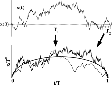
Figure 1: Schematic illustration of the definition of the average shape of a fluctuation. Above, the signal $x(t)$ is shown and two successive positive fluctuations above $x(0)$ are indicated. Below the two fluctuations are rescaled and compared to the average shape.

In this Letter we compute this average trajectory for stochastic processes of the form

$$x(t+1)=x(t)+\xi(t)$$ (1)

with $x(0)=0$ nota . The increment $\xi(t)$ is a random variable. Despite the simplicity of the processes considered, we uncover a rich phenomenology. We find that, in all cases considered, a scaling law is obeyed

$$\langle x(t)\rangle_{T}=T^{\alpha}f(t/T),$$ (2)

in appropriate time regimes. The value of the exponent $\alpha$ results to be equal to the wandering exponent of the “free” process (i. e. not constrained to return to 0 at time $T$, nor to be always positive). The scaling function $f(s)$ turns out instead to be a sensitive probe of temporal correlations of the dynamical process, while it is to a large extent independent on the statistics of single increments. In particular, for uncorrelated noise the scaling function is always proportional to a semicircle. For correlated noise the tails are universal with respect to the single step distribution, and they depend only on the short- or long-ranged nature of the correlations.

We consider processes of the form (1) and focus our attention on the trajectory of a walk originating in $x(0)=0$ at time $0$ and returning to $x(0)$ for the first time at time $T$, known in the mathematical literature as excursion. We first study the case of uncorrelated random walks and Levy flights and then move to the analysis of the effect of correlations.

i) Gaussian walks: The simplest process of this kind is the uncorrelated unbiased random walk, where $\langle\xi(t)\rangle=0$ and $\langle\xi(t)\xi(t^{\prime})\rangle=\delta_{t,t^{\prime}}$. By using the time-reversal symmetry the average trajectory can be written as

$$\langle x(t)\rangle_{T}={\int_{0}^{\infty}dx\,\,x\,\,F(x,t)F(x,T-t)\over\int_{0}^{\infty}dx\,\,F(x,t)F(x,T-t)}.$$ (3)

where $F(x,t)$ is the probability that a walker starting in $x=0$ at time $0$ reaches $x$ at time $t$ without ever touching the axis $x=0$.

If we consider a normal distribution for single steps $F(x,t)$ can be determined via the image method Rednerbook . The result for $\langle x(t)\rangle_{T}$ is of the form (2) with $\alpha=1/2$ and scaling function proportional to a semicircle long

$$f_{U}(s)=\sqrt{8\over\pi}\sqrt{s(1-s)}.$$ (4)

The exponent $\alpha$, being equal to the value characterizing a free walk, indicates that the constraint of returning at time $T$ does not affect the amplitude of the excursion. The same value of $\alpha$ and the same expression (4) for $f(s)$ are expected for any distribution of single steps $P(\xi)$ with finite variance, for which central limit theorem holds. Eq. (4) can be easily computed explicitly in the case of a bimodal $P(\xi)$.

To extend our analysis to other processes we resort to numerical simulations for the evaluation of $\langle x(t)\rangle_{T}$. We consider walks starting at $x=0$ at some negative time, and we take as $t=1$ the first time such that $x(t)>\epsilon$, where $\epsilon$ is a small positive threshold. We average over all walks that first return between $[-\epsilon,\epsilon]$ at a specified time $T$, under the constraint $x(t)>\epsilon$ for $1<t<T$. For each time $T$ the average shape is normalized by the factor $N(T)=\int_{0}^{1}ds\langle x(sT)\rangle_{T}$. If the scaling form (2) holds, the normalized shapes for different $T$ collapse on a single curve and $N(T)$ grows as $T^{\alpha}$. We average from $10^{4}$ to $10^{7}$ pulses for each $T$. However, as shown in experiments Mehta01 , smaller statistics ($\approx 10^{3}$ pulses) is already sufficient for reasonably clean curves.

ii) Levy flights: While it is well known that random walks with finite variance of the step distribution belong to the Gaussian universality class, distributions with fat power-law tails give rise to a completely different behavior Bouchaud90 . For this reason we consider now process (1) where the distribution of independent increments $\xi$ has infinite variance, i.e. with tails decaying as $P(\xi)\propto|\xi|^{-\mu-1}$ where $0<\mu<2$. Although $\langle x(t)\rangle_{T}$ can still be written in the form (3), $F(x,t)$ can not be computed by the image method. We find numerically that also in this case the scaling form (2) is obeyed, with $\alpha=1/\mu$ and the scaling function $f(s)$ of the same semicircular shape (4) of the case with finite variance. This holds for any $\mu>0$ (in Fig. 2 we show $\langle x(t)\rangle_{T}$ for $\mu=0.7$), thus even regardless the existence of the first (absolute) moment of the single step distribution notaCauchy .

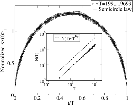
Figure 2: Main: Plot of the normalized average fluctuation $\langle x(t)\rangle_{T}$ for a random walk with power-law distributed steps with $\mu=0.7$. The solid line represents the universal function (4). Small circles are for several values of $T$ ranging from 199 to 9699. Inset: Plot of the normalization factor $N(T)$, which scales as $T^{1/\mu}$, indicating that $\alpha=1/\mu$. The dashed line is proportional to $T^{1/\mu}$.

While a scaling exponent $\alpha$ equal to the wandering exponent of the free process could be expected notaalpha , the fact that the shape of the scaling function remains exactly the same is surprising. Note that the short time expansion of Eq. (2)

$$\langle x(t)\rangle_{T}\propto T^{1/\mu-1/2}\,\,t^{1/2}$$ (5)

in the Gaussian case $\mu=2$ gives $\langle x(t)\rangle_{T}\propto t^{1/2}$, equal to the wandering of the unconstrained walk. One could naively expect by analogy a short time behavior as $t^{1/\mu}$ for $\mu<2$ (corresponding to the free walk). Eq. (5) shows that this is not the case, indicating that the Levy flight feels the constraints even for short times.

Universality in the shape of the scaling function is not restricted to changes of the variance $\langle\xi^{2}\rangle$ of the single step distribution. Also variations of the mean value $\langle\xi\rangle$, corresponding to the addition of a bias to the walk, do not modify $f(s)$. This is easily shown analytically in the case of gaussian or bimodal $P(\xi)$ and has been checked numerically for the other cases. Therefore we can conclude that, for all processes of the type (1) with uncorrelated noise, the scaling function $f(s)$ is proportional to a semicircle.

iii) Walk in a parabolic well: A further generalization is to consider a walk in a harmonic potential

$$x(t+1)=x(t)-\lambda x(t)+\xi(t)$$ (6)

where the term $\lambda x$ describes the effect of a parabolic well. The damping $\lambda$ introduces a characteristic time, of order $1/\lambda$, so that scaling breaks down for large times. The probability for the walker to return at time $T$, i. e. the distribution of return times $P(T)$, remains the same ($\propto T^{-3/2}$) for $T\ll 1/\lambda$, while it decays exponentially for $T\gg 1/\lambda$. Also for this process the average fluctuation can be computed analytically via the image method and is long

$$\langle x(t)\rangle_{T}=\sqrt{{4\over\pi\lambda}{(1-e^{-2\lambda t})(1-e^{-2\lambda(T-t)})\over(1-e^{-2\lambda T})}}$$ (7)

Figure 3: Average excursion for a random walk in a parabolic well [Eq. (7)] for $1/\lambda=20$. From top to bottom lines are for $T=10,25,50,100,250$. Notice that the shape flattens to the constant value $\sqrt{4/(\pi\lambda)}$ (thin line).

As shown in Fig. 3, for $T\ll 1/\lambda$ we get a semicircle, the same result as for $\lambda=0$. For larger $T$ instead, as correlations decay, the form of the fluctuation tends to become flat, while keeping the $(t/T)^{1/2}$ ($(1-t/T)^{1/2}$) behavior at the left (right) tail. This is strongly reminiscent of the flattening observed experimentally by Durin and Zapperi in the study of the Barkhausen noise in magnetic systems Durin02b : indeed, in that case the damping term is provided the demagnetizing field, which controls the cutoff in the avalanche distribution Zapperi98 .

So far we have considered processes with increments $\xi(t)$ extracted independently at each time step. Let us now analyze the effect of temporal correlations in the stochastic noise. More precisely, we consider processes such that

$$g(t,t^{\prime})\equiv\langle\xi(t)\xi(t^{\prime})\rangle-\langle\xi(t)\rangle\langle\xi(t^{\prime})\rangle\neq\delta_{t,t^{\prime}}.$$ (8)

iv) Short-ranged memory: Let us first study the case of noise with correlations decaying exponentially over some interval $\tau$, i.e. $g(t,t^{\prime})=\exp{(-|t-t^{\prime}|/\tau)}$. The average fluctuation for this process, evaluated numerically, is reported in Fig. 4, showing the existence of two regimes. When $T\approx\tau$ the shape of $\langle x(t)\rangle_{T}$ is parabolic, similarly to what has been observed in Mehta01 for the random field Ising model. The detailed form depends on the distribution of single steps $P(\xi)$ and in particular it is skewed for power-law distributed $\xi$. However, some form of universality with respect to $P(\xi)$ is present also in this case: The tails of $\langle x(t)\rangle_{T}$, which go to zero linearly both for small $s$ [Fig. 4, inset] and for $s\to 1$ (not shown). In the long time limit $T\gg\tau$, memory in the noise is lost and, as expected, we recover the semicircular shape (Fig. 4), that characterizes processes with uncorrelated increments.

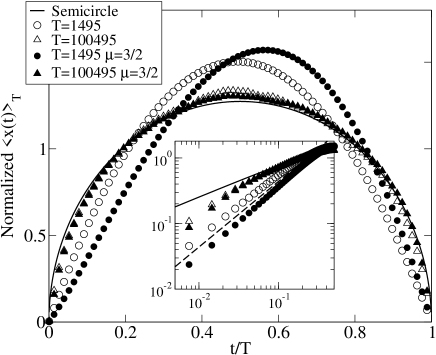
Figure 4: Main: Plot of the normalized average fluctuation $\langle x(t)\rangle_{T}$ for a random walk fed by noise with short time memory ($\tau=1000$). Empty symbols are for uniformly distributed $\eta$, while the filled ones are for power-law distributed $\eta$ with $\mu=3/2$. Circles are for a time of the order of $\tau$, while triangles are for $T\gg\tau$. The solid line represent the universal function (4) after normalization. Inset: The tails for small $t/T$ of the same curves of the main panel plus a straight dashed line of slope 1.

v) Long-ranged memory: We finally analyze a stochastic process with long-ranged memory, given by Eq. (1), where now $\xi(t)=\sum_{i=1,t}\eta(i)$ and $\eta(i)$ is an uncorrelated noise. This process can be seen as a temporally discrete version of the continuous process $\partial_{t}^{2}x=\eta(t)$, which is known as the random accelerated particle (RAP) and has been studied in the context of inelastic collapse of granular matter Cornell98 . For a distribution of $\eta(t)$ with unitary variance the correlation function of $\xi(t)$ is $g(t,t^{\prime})=\min(t,t^{\prime})$ and hence it does not decay when the difference between $t$ and $t^{\prime}$ grows. The first return probability to the origin of the walker has been recently shown analytically to decay as $P(T)\propto T^{-5/4}$ Sinai92 . By evaluating numerically the average fluctuation $\langle x(t)\rangle_{T}$ we recover also in this case the scaling form [Eq. (2)], with $\alpha=3/2$, that again corresponds to the wandering exponent for the unconstrained process. The normalized scaling function, plotted in Fig. 5, is indistinguishable from the simple curve

$$f(x)={x^{3/2}(1-x)\over B(3/2,1)}$$ (9)

where $B$ is the Beta function.

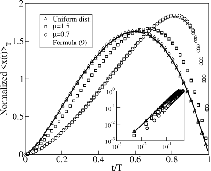
Figure 5: Main: Plot of the normalized average fluctuation $\langle x(t)\rangle_{T}$ for the random accelerated particle. Triangles are for uniformly distributed $\eta$, while squares and circles are for power-law distributed $\eta$, respectively with $\mu=1.5$ and $\mu=0.7$. The values of $T$ range from 1000 to 100000. Inset: The tails for small $t/T$ of the same curves of the main panel plus a straight line of slope 3/2.

For a RAP with power-law distributed $\eta$ (infinite variance), the exponent $\alpha$ is $1+1/\mu$ (again as in the free case). As in the case with short-ranged correlations the scaling function differs from the case with finite variance (Fig. 5), and the asymmetry is more evident for small $\mu$. Nevertheless the behavior of the tails remains universal, being $f(s)\propto s^{3/2}$ for $s\to 0$ (see Fig. (5), inset) and $f(s)\propto 1-s$ for $s\to 1$ (not shown).

In conclusion, we have tackled theoretically the problem of analyzing generic time series from the point of view of the average shape of their fluctuations. In particular, we have studied this quantity for stochastic processes of the form (1). We find that the scaling law $\langle x(t)\rangle_{T}=T^{\alpha}f(t/T)$ is obeyed in an appropriate time regime. The exponent $\alpha$ coincides with the wandering exponent of the unconstrained process, as can be expected on the basis of scaling arguments. More interestingly, the scaling function $f(s)$ exhibits some degree of universality. For any process with uncorrelated increments $f(s)$ is proportional to a semicircle, with no dependence whatsoever on the distribution of single steps. Modification of this shape can be obtained only via additional $x$-dependent terms in Eq. (1) or introducing correlations in the stochastic increments. In this last case, the average fluctuation is in general asymmetric and, although its detailed shape depends on the distribution of single increments, the tails are universal, depending only on the short- or long-ranged nature of noise correlations. Because different universal behaviors encode solely correlation properties of the signal, this quantity is a powerful tool in the statistical analysis of temporal series: In many systems it would be very interesting to compare quantitatively $\langle x(t)\rangle_{T}$ between experiments and models in the light of our results. In the case of Barkhausen noise, where this comparison has pointed out the limitations of current models, our study provides a guide for refining them in order to better capture the physics of the phenomenon.

We are grateful to Lorenzo Bertini for an interesting discussion, to Alan Bray for useful correspondence, and to Stefano Zapperi for a critical reading of the manuscript. F. C. is supported by the INFM PAIS-G project “Hysteresis in disordered ferromagnets”.

References

- (1) J. P. Sethna, K. A. Dahmen, and C. R. Myers, Nature, 410, 242 (2001).
- (2) G. Bertotti, Hysteresis in Magnetism (Academic Press, San Diego, 1998).
- (3) E. T. Lu, R. J. Hamilton, J. M. McTiernan, and K. R. Bromond, Astrophys. J. 412, 841 (1993).
- (4) E. R. Kanasewich, Time Sequence Analysis in Geophysics (University of Alberta Press, Edmonton, 1981).
- (5) J. P. Bouchaud and M. Potters, Theory of Financial Risk: From Statistical Physics to Risk Management (Cambridge University Press, Cambridge, 2000).
- (6) M. C. Kuntz and J. P. Sethna, Phys. Rev. B 62, 11699 (2000).
- (7) G. Durin and S. Zapperi, J. Magn. Magn. Mat. 242-245P2, 1085 (2002).
- (8) A. P. Mehta, A. C. Mills, K. Dahmen, and J. P. Sethna, Phys. Rev. E 65, 046139 (2002).
- (9) In all processes considered here the results are easily shown to be independent from the choice of , except for process (6), that will be discussed elsewhere long . However, one may in general expect that changing will affect the average excursion as it does for other statistical properties, e.g. the first-return probability.
- (10) S. Redner A Guide To First-Passage Processes (Cambridge University Press, Cambridge, 2001).
- (11) F. Colaiori, A. Baldassarri and C. Castellano (in preparation).
- (12) J. P. Bouchaud and A. Georges, Phys. Rep. 195, 127 (1990).
- (13) To corroborate the results presented in Fig. 2 we have computed numerically for the Cauchy distribution, which is the Levy-stable process for . The result agrees extremely well with the ansatz , where is a normalization constant. Interestingly, using this form for in Eq. (3) and performing the integrals, we recover .
- (14) For all processes such that the average trajectory can be written in the form Eq. (3), it is enough to assume a scaling form for the conditional probability to have .
- (15) G. Durin and S. Zapperi, (unpublished).
- (16) S. Zapperi, P. Cizeau, G. Durin, and H. E. Stanley, Phys. Rev. B 58, 6353 (1998).
- (17) S. J. Cornell, M. R. Swift, and A. J. Bray, Phys. Rev. Lett. 81, 1142 (1998).
- (18) Y. G. Sinai, Theor. Math. Phys., 90 219 (1992); T. W. Burkhardt, J. Phys. A 26, L1157 (1993).