Testing of two-dimensional local approximations in the current-spin and spin-density-functional theories.

Abstract

We study a model quantum dot system in an external magnetic field by using both the spin-density-functional theory and the current-spin-density-functional theory. The theories are used with local approximations for the spin-density and the vorticity. The reliabilities of different parametrizations for the exchange-correlation functionals are tested by comparing the ensuing energetics with quantum Monte Carlo results. The limit where the vorticity dependence should be used in the exchange-correlation functionals is discussed.

I Introduction

The success of the spin-density-functional theory (SDFT) [1] within the local-spin-density approximation (LSDA) to predict accurate results for the electronic structure of two-dimensional quantum dot systems depends on the exchange-correlation functionals used. Until recently, functionals based on the diffusion quantum Monte Carlo (DMC) calculations by Tanatar and Ceperley [2] have been widely employed. The simulations were performed for the spin-compensated and spin-polarized two-dimensional electron gas (2DEG). Recently, Attaccalite et al. [3, 4] made fixed-node DMC calculations with improved accuracy for the 2DEG including several partial spin-polarizations. They provided interpolation formulas which fulfil several exact results at the low and high electron density limits.

In the current-spin-density-functional theory (CSDFT), used to describe electron systems in magnetic fields, the exchange-correlation energy depends also on the paramagnetic current density [5]. In the local approximation the current-dependence is converted to the dependence on the vorticity or on the Landau-level filling factor. The low filling factor (strong magnetic field) limit for the totally spin-polarized electron gas, is well known from the works by Levesque, Weis and MacDonald [6], Fano and Ortolani [7], and Price and Das Sarma [8]. The problem is how to interpolate the exchange-correlation energy between this limit and the high filling factor (zero-magnetic field) limit for a given spin-polarization. Several interpolation schemes have been suggested [9, 10, 11].

The purpose of the present work is to study the reliabilities of the two zero-field exchange-correlation functionals and various exchange-correlation interpolation schemes with respect to the filling factor in the CSDFT calculations. We use a parabolically-confined quantum dot as the test system and compare our SDFT and CSDFT total energies with those obtained in variational quantum Monte Carlo (VMC) calculations [12, 13]. In the zero-field case the parabolic confinement is lowered towards the limit of Wigner-crystallization and the difference between the total energies of the spin-polarized and spin-compensated solutions are monitored. For a finite confinement we calculate the ground state energy as a function of the external magnetic field. Besides the CSDFT schemes, calculations are performed also with the SDFT, i.e ignoring the current-dependence of the exchange-correlation energy. Thus, our calculations enlighten how important improvement the CSDFT is in comparison with the SDFT. For the quantitative comparisons we need numerically accurate results. We perform the SDFT and CSDFT calculations on two-dimensional point grids imposing no symmetry restrictions [13, 14]. The convergence with respect to the grid size and other numerical approximations is carefully tested. The VMC results are converged beyond the statistical noise.

The outline of the present paper is as follows. In Sec. II we shortly describe the exchange-correlation functionals in zero magnetic field and give our results for a six-electron quantum dot as a function of the confinement. In Sec. III we discuss the interpolation as a function of the Landau level filling factor and show our results for the magnetic field dependence on the ground-state total energy. Sec. IV contains the conclusions. Effective atomic units are used in the formulas throughout the paper and for presenting the results they are converted by using the material parameters of GaAs, i.e. the dielectric constant $\epsilon=12.4$, the effective mass $m^{*}=0.067$ and the gyromagnetic constant $g^{*}=-0.44$. We choose the coordinate system so that $x$ and $y$ are in the plane of the dot and the $z$-axis is perpendicular to the plane.

II zero-field and the low-density limit

Attaccalite et al. (AMGB) [3, 4] calculated the ground state of the 2DEG with the fixed-node DMC. Compared to the work by Tanatar and Ceperley (TC)[2] there are a number of improvements in the numerical calculations. Backflow correlations in many-body wave functions are included, and infinite size extrapolations are performed in the Monte Carlo data. An important new feature of the results by Attaccalite et al. is the appearence of a spin-polarized ground state before the Wigner crystallization.

On the basis of their DMC calculations, AMGB [3] proposed a new analytic representation of the correlation energy. It takes into account several exact results in the low and high density limits. They give the exchange-correlation energy of the homogeneous electron gas as

$$e_{\rm xc}(r_{s},\zeta)=e_{x}(r_{s},\zeta)+(e^{-\beta r_{s}}-1)e_{\rm x}^{(6)}(r_{s},\zeta)+\alpha_{0}(r_{s})+\alpha_{1}(r_{s})\zeta^{2}+\alpha_{2}(r_{s})\zeta^{4}.$$ (1)

Here $r_{s}=1/\sqrt{\pi n}$ is the density parameter, calculated from the two-dimensional electron density $n$, and $\zeta=(n_{\uparrow}-n_{\downarrow})/n$ is the spin polarization determined by the spin-up and spin-down electron densities $n_{\uparrow}$ and $n_{\downarrow}$, respectively. $e_{x}(r_{s},\zeta)$ is the exchange energy, which can be written as

$$e_{\rm x}(r_{s},\zeta)=-2\sqrt{2}[(1+\zeta)^{3/2}+(1-\zeta)^{3/2}]/3\pi r_{s}.$$ (2)

In Eq. (1), $e^{(6)}_{\rm x}$ contains the terms of the Taylor expansion of $e_{\rm x}$ with respect to $\zeta$ at $\zeta=0$ which are beyond the fourth order in $\zeta$, $\alpha$’s are density dependent functions of the generalized Perdew-Wang form[15], and $\beta=1.3386$.

The above form (1) is based on DMC calculations for partial polarizations ($0<\zeta<1$). TC [2] made DMC calculations only for spin-compensated ($\zeta=0$) and spin-polarized ($\zeta=1$) systems. To calculate the correlation potential for finite polarizations the TC data is often used with the exchange-like interpolation[16] of Eq. (2). This leads to deviations from the exact results at high electron densities and too small spin-susceptibilities at low densities [3].

Our test system is a six-electron quantum dot confined by a parabolic external potential

$$V_{\rm ext}={1\over 2}m^{*}\omega^{2}_{0}r^{2},$$ (3)

where $\hbar\omega_{0}$ is the confinement strength. First we use a zero magnetic field and compare the results obtained with the two LSDA functionals to the VMC results. We study the weak-confinement limit at which the electron density in the dot is low and therefore the contribution of the exchange-correlation energy to the total energy is relatively large. Thus, the high-correlation effects in this particular system, i.e. the Wigner crystallization, spin density wave (SDW) formation, and spin-polarization, are assumed to be sensitive to the LSDA functional used.

Fig. 1 shows the energy difference between the $S_{z}=3$ and $S_{z}=0$ spin states as a function of the confinement strength. The agreement with the VMC results is remarkably better for the AMGB functional than for the TC parametrization. In the AMGB results the spin-polarization is favoured at confinement strengths below $\hbar\omega_{0}=0.23$ meV. This is roughly in the middle between the TC and VMC results of 0.18 and 0.28 meV, respectively. As the confinement is made stronger, the difference between the parametrizations grows further enhancing the advantage of the new LSDA so that it smoothly follows the VMC curve. The origin of the difference is in the total energy of the polarized ($S_{z}=3$) state. It is lowered when the AMGB functional is used instead of the TC one. This observation is in accord with the result of Gori-Giorgi et al. [4] that the improvement due to the new functional is directly proportional to the polarization and the electron density of the system. In the present case, however, there is a significant difference between these two approximations down to $\hbar\omega_{0}\simeq{0.15}$ meV. This corresponds to quite a small electron density, i.e. $r_{s}=(N^{1/4}\hbar\omega_{0})^{-2/3}\sim 14$ (Ref. [16]). In our calculations, this is actually the smallest confinement strength for which we have strictly converged SDFT results.

The transition point to the $S_{z}=0$ SDW state also seems to depend strongly on the applied type of LSDA. By using the TC functional we find the breaking of the spin symmetry at $\hbar\omega_{0}\simeq{0.45}$ meV, whereas with the new LSDA the transition occurs already at $\hbar\omega_{0}\simeq{0.8}$ meV, which corresponds to $r_{s}=4.5$. This should be compared with the estimation by Koskinen et al. that in the case of closed shells, a SDW is found for $r_{s}\gtrsim{5}$ (Ref. [16]). Fig. 1 shows also the results obtained by forcing the spin densities to be equal, i.e. preventing the SDW formation. It can be seen that the values of the SDW solutions are in a clearly better agreement with the VMC results than those of the symmetry-restricted solution. The relative amplitude of the SDW grows rapidly at low confinements below the transition point, and the electron density shows localization around six maxima, corresponding to the Wigner crystallization. The behavior of the electron density is presented in more detail in Ref. [13].

III External magnetic field

Next we add an external magnetic field perpendicular to the dot (i.e. parallel to the $z$-axis) and fix the confinement strength to $5\;{\rm meV}$. SDFT calculations are done with a minimal substitution of the external vector potential in the Schrödinger equation, and by using the zero-field exchange-correlation functionals for the 2DEG. In the CSDFT [5] the exchange-correlation functionals depend on the electron currents in the system, and they are functionals of the spin densities and the vorticity,

$$\gamma({\bf r})=\nabla\times{{\bf j}_{p}({\bf r})\over n({\bf r})}\biggr{|}_{z}.$$ (4)

Above, $n$ is the electron density and ${\bf j}_{p}$ is the paramagnetic current density. Equally, we can use the Landau level filling factor given by

$$\nu=2\pi n/\gamma.$$ (5)

The data for the 2DEG in magnetic field is scarce. Fano and Ortolani [7] used the Monte Carlo data by Morf et al. [17] and gave the $\nu$ dependence of the 2DEG exchange-correlation energy for low $\nu$ values from 0 to about 0.8, corresponding to high magnetic fields. At the limit of the infinite magnetic field ($\nu\rightarrow 0$), the resulting curve agrees well with the results by Levesque, Weis, and MacDonald [6]. Price and Das Sarma[8] obtained for the polarized 2DEG the density dependence of the exchange-correlation energy at the $\nu$ values of 1/7, 1/5, 1/3, 1 and 2. In the low $\nu$ region the fractional quantum Hall effect causes cusps in the exchange-correlation energy. Heinonen et al. [10] took them into account in their modeling, but we have ignored them because in our test case of the six-electron quantum dot, the $\nu$ values were above 0.9 in the magnetic fields up to 10 T.

In the present calculations we have used expressions given by Koskinen et al.[11] and Ferconi and Vignale [18] for the magnetic-field dependence of the exchange-correlation (See also Ref. [9]). Koskinen et al. fitted their functionals in the high vorticity limit and used the following formula for the interpolation to the zero-field limit,

$$e^{\rm K}_{\rm xc}(n,\zeta,\nu)=-0.782\sqrt{2\pi n}e^{-f(\nu)}+e^{B=0}_{\rm xc}(n,\zeta)(1-e^{-f(\nu)}),$$ (6)

where $f(\nu)=1.5\nu+7\nu^{4}$. Koskinen et al. used the TC functional as the zero-field limit $e_{\rm xc}^{\rm B=0}$. We replace it by the AMGB functional (Eq. (1)). Ferconi and Vignale applied a Padé approximant, fitting the low $\nu$ limit of Levesque et al. [6] to the zero magnetic field functionals, i.e.,

$$e^{\rm PADE}_{\rm xc}(n,\zeta,\nu)=(e^{\rm LWM}_{\rm xc}(n,\nu)+\nu^{4}e^{B=0}_{\rm xc}(n,\zeta))/(1+\nu^{4}),$$ (7)

where $e^{\rm LWM}_{\rm xc}$ is the interpolation formula for the infinite magnetic field limit [6],

$$e^{\rm LWM}_{\rm xc}=-0.782133\sqrt{2\pi n}(1-0.211\nu^{0.74}+0.012\nu^{1.7}).$$ (8)

As before, we insert the AMGB functional for $e_{\rm xc}^{\rm B=0}$. The above formulae interpolate between the fully polarized electron gas values at high magnetic fields and the zero-field limit, which may have arbitrary polarization. Data for the intermediate polarizations at high magnetic fields would be desirable to test the interpolation further.

Fig. 2(a) shows the quantum Monte Carlo data by Price and Das Sarma [8] and Fano and Ortolani[7] for the exchange-correlation energy of the polarized 2DEG at $n=0.138$ a.u. The horizontal line indicates the zero-field limit of AMGB. Fig. 2(a) shows also values from exchange-correlation energy by Koskinen et al. (Eq. (6)). At low $\nu$ values all the data agree well but when $\nu$ increases the results by Price and Das Sarma ($\nu=1$ and $\nu=2$) approach much more slowly the zero-field limit than the data by Fano and Ortolani. Therefore we propose a new functional which is an interpolation to the data by Price and Das Sarma. The resulting functional is

$$e^{\rm{new}}_{\rm xc}(n,\zeta,\nu)=(e^{\rm LWM}_{\rm xc}(n,\nu)+\nu^{4}e^{B=0}_{\rm xc}(n,\zeta))/(1+0.0061\nu-0.0314\nu^{2}-0.0201\nu^{3}+\nu^{4}),$$ (9)

and it is shown in Fig. 2(b). In the same figure we have also plotted $e^{\rm PADE}_{\rm xc}$ of Ferconi and Vignale. One should note that at $\nu<1$ it approaches the zero-field limit much more slowly than the data by Fano and Ortolani in Fig. 2(a). The $e^{\rm PADE}_{\rm xc}$ shows a maximum above the zero-field values, for which there is, however, no physical reason.

The exchange-correlation potential $V_{\rm xc}$ is obtained in the local approximation by calculating the functional derivative

$$V_{{\rm xc},\sigma}(n_{\uparrow},n_{\downarrow},\nu)=\partial(ne_{\rm xc})/\partial n_{\sigma}.$$ (10)

In the CSDFT, the vector potential depends on the derivative with respect to the vorticity. The $x$ and $y$ components of the exchange-correlation vector potential ${\bf A}_{\rm xc}$ are

$$A_{{\rm xc},x}=1/n{\partial\over\partial y}{\partial(ne_{\rm xc})\over\partial\gamma},$$ (11)

$$A_{{\rm xc},y}=-1/n{\partial\over\partial x}{\partial(ne_{\rm xc})\over\partial\gamma}.$$ (12)

It should be noted that the contribution of the exchange-correlation energy to the total energy arises via the value of $e_{\rm xc}$ at the given density and vorticity and via its derivatives with respect to both density and vorticity. Therefore the total energies are sensitive to even slight variations in the exchange-correlation functionals.

The vorticity is a functional of the ratio between the paramagnetic current density and the electron density (Eq. (4)). Its values increase rapidly towards low density areas causing numerical instabilities. To circumvent them we have used the convoluted form of Koskinen et al. [11] in the calculation of the partial derivatives $\partial e_{\rm xc}/\partial\gamma$ in Eqs. (11) and (12),

$${\partial e_{\rm xc}\over\partial\gamma}\approx\int{(\gamma^{\prime}-\gamma)\over\sqrt{2\pi}\Delta^{3}}e^{-(\gamma^{\prime}-\gamma)^{2}\over 2\Delta^{2}}e_{\rm xc}(n,\zeta,\gamma^{\prime}).$$ (13)

Above, the width $\Delta$ of the Gaussian function should be carefully adjusted to the vorticity of the system at the given magnetic field strength. Too small values for $\Delta$ may result in convergence problems. On the other hand using too large a value for $\Delta$ may cause inaccuracy in the results. In our calculations $\Delta$ ranges from 0.025 to 0.05.

Fig. 3 shows the total ground state energy of a six-electron dot as a function of the magnetic field up to 10 T. Results obtained with the SDFT and CSDFT formalisms and different functionals are compared with the VMC data. Assuming again that the VMC results follow most faithfully the exact ones, the CSDFT formalism is a clear improvement over the SDFT formalism: The CSDFT results obtained with the AMGB functional using the Padé approximant for the filling factor interpolation, are closer to the VMC values than the SDFT values already at magnetic fields slightly above 2 T. In this region $S_{z}=0$. The improvement of the CSDFT formalism is also clear above 5 T, where $S_{z}=3$ and the maximum density droplet (MDD) has been formed. The use of the AMGB functional instead of the TC functional improves the SDFT results in the regions of large spin polarization, i.e., around $B$ = 4.5T where $S_{z}=2$, and in the MDD region. This conclusion matches again well with the analysis by Gori-Giorgi et al. [4].

In the CSDFT, the ground state energy depends clearly on the chosen exchange-correlation functional. As shown in Fig. 3 the interpolation suggested by Koskinen et al. (Eq. 6) does not cause a big difference between the CSDFT and SDFT results. This is because $e^{\rm K}_{\rm xc}$ saturates quickly to the zero-field values at about $\nu=1$ due to the exponential factors. The clear difference obtained by using the Padé approximant (Eq. (8)) with an increasing magnetic field results in a much better agreement with the VMC data. Second, the results obtained with the AMGB functional coincide well in the MDD region with the VMC ones, whereas those obtained with the TC functional (not shown in Fig. 3) are higher in energy resembling the situation in the SDFT calculations. Third, the new functional (Eq. (9)) based on the data by Price and Das Sarma seems to overcorrect the SDFT results. We conclude that despite the good fit to the Monte Carlo data for polarized 2DEG, the derivatives of $e_{\rm xc}$ seem to be poorly approximated by Eq.(9) as well as the spin compensated $\zeta=0$ values for $e_{\rm xc}$.

In the MDD region of the VMC results the $S_{z}=2$ state constitutes the ground state in the CSDFT calculations for the exchange-correlations energies given in Eqs. (7) and (9). The corresponding energies are given in Fig. 3 as x-marks and dots, respectively. However, we believe that the $S_{z}=2$ groundstate is an artifact due to the interpolation of the exchange-correlation energy between the high-field totally-polarized and the zero-field partially-polarized electron gas values. Due to lack of simulation data the polarization dependence enters the exchange-correlation functionals only through the zero-field limits in Eqs. (6), (7), and (9). The high-field $S_{z}=2$ CSDFT ground states have the same value for the total angular momentum, $L_{z}=15$, as for the $S_{z}=3$ MDD-state, but the electron at the innermost orbital has a flipped spin. Therefore, Hund’s rule should favor the totally polarized $S_{z}=3$ state. Further, we see that also around $B$ = 4.5T, where both the CSDFT and VMC give the $S_{z}=2$ state, the CSDFT clearly underestimates the total energy.

IV conclusions

We have studied the electronic structure of a parabolically-confined six-electron quantum dot using the spin-density-functional and the current-spin-density-functional theories. In particular the effects of weak confinement and strong external magnetic field were considered. Our main aim was to investigate, how reliably the different local approximations for the electron exchange and correlation follow variational quantum Monte Carlo results, which we consider as benchmarks. We have especially investigated the various interpolation schemes between the spin-compensated and totally polarized electron gas and the vorticity dependence of the exchange-correlation functionals.

We find that the new LSDA functional by Attaccalite et al. gives in the zero magnetic field much better results for the total energy than the old form by Tanatar and Ceperley. According to our results, the same is also true in an external magnetic field for a six-electron quantum dot with a typical confinement of $\hbar\omega_{0}$ = 5 meV. For this system the effect of currents on the exchange-correlation energy becomes important in magnetic fields larger than 2 - 3 T. In our calculations for these high magnetic fields the local Landau level filling factor $\nu$ is of the order of 0.9. The simulation data for the homogeneous electron gas in this regime is scarce, which hampers establishing of interpolation forms between the low and high magnetic field limits (large and small Landau level filling factors). The Padé interpolation by Ferconi and Vignale gives a very good agreement with the quantum Monte Carlo results in the case of spin-compensated and spin-polarized states of our system. The exponential interpolation form by Koskinen et al. underestimates clearly the effect of the magnetic field. Our results for the partially spin-polarised states in magnetic field are remarkably worse than those for the spin-compensated and spin-polarized states. Thus, our tests with the CSDFT call for further simulations for the homogeneous electron gas in order to determine reliable interpolation forms for the vorticity and polarization dependence of the exchange-correlation functionals.

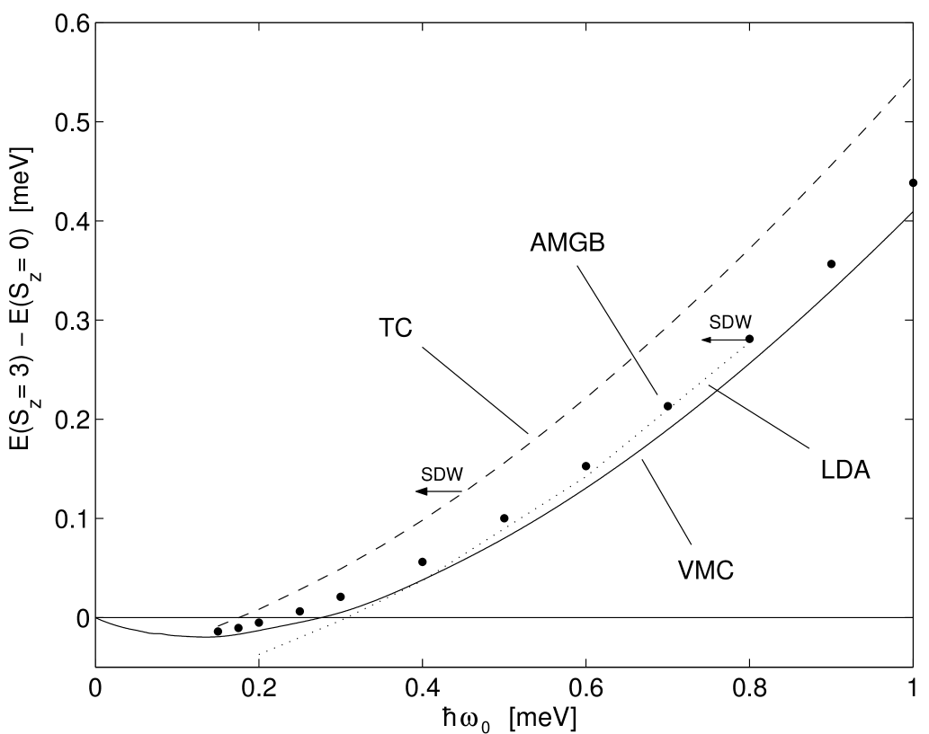
FIG. 1.: Total energy difference between the $S_{z}=3$ and $S_{z}=0$ spin states in a six-electron quantum dot. The results obtained with the SDFT using the LSDA functionals by TC [2] and AMGB [3] are compared with the VMC data. The onsets of SDW solutions with decreasing confinement are marked by arrows. The dotted curve shows the symmetry-restricted results, corresponding to the LDA.

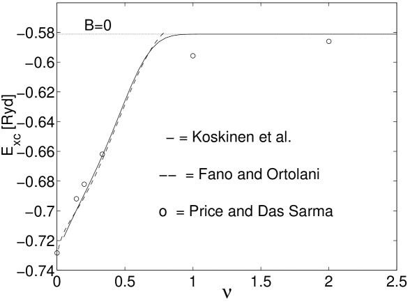
(a)

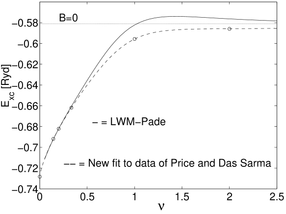
(b)

FIG. 2.: Exchange-correlation energy per electron as a function of the Landau level filling factor for the spin-polarized 2DEG with $n=0.138$ a.u. (a) Monte Carlo simulation data calculated by Price and Das Sarma [8] (open circles), and the interpolation forms by Fano and Ortolani [7] and Koskinen et al. [11] (Eq. (6)). The zero-field limit by AMGB is shown by the dotted line. (b) Data of Price and Das Sarma [8], the Padé approximant used by Ferconi and Vignale [18] (Eq. (7)) and the new fit (Eq. (9)) to the data of Price and Das Sarma $e^{\rm new}_{\rm xc}$.

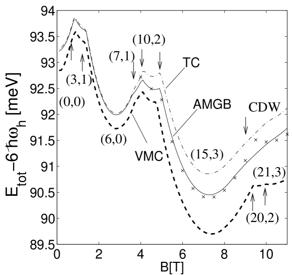
(a)

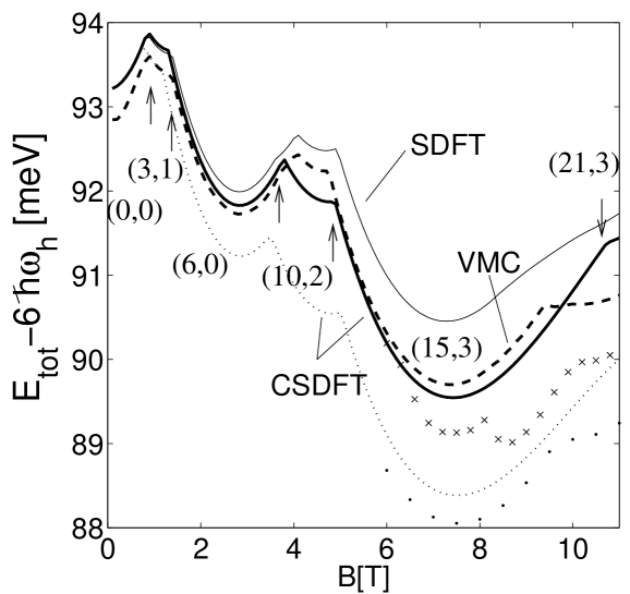
(b)

FIG. 3.: Ground state energy (minus $6\;\hbar\omega_{h}=6\;\hbar\sqrt{\omega_{0}^{2}+(\omega_{c}/2)^{2}}$, where $\omega_{c}=eB/m^{*}$ is the cyclotron frequency) for the six-electron quantum dot in parabolic confinement with the strength $\hbar\omega_{0}=5\textrm{ meV}$. (a) SDFT results using the AMGB (solid line) and TC (dash-dotted line) functionals. The VMC results are marked with the bold dashed line. The x-marks denote the CSDFT results obtained using the exchange-correlation functional by Koskinen et al. (Eq. (6)). CDW denotes charge density wave state which breaks the rotational symmetry. (b) CSDFT results using the exchange-correlation interpolations by Ferconi and Vignale (Eq. (7)) (bold solid line) and the new functional (Eq. (9)) (dotted line). The best SDFT results are repeated (solid line). The zero-field AMGB exchange-correlation functional has been used in these calculations. The x-marks and dots denote the CSDFT results for the $S_{z}$ = 2 state obtained using the Ferconi and Vignale functional and the new functional, respectively. The z-components of the total spin and and the total angular momentum are given in parenthesis as ($L_{z}$, $S_{z}$) and arrows mark the transition points. It should be noted that the (7, 1) state is missing in CSDFT.

REFERENCES

- [1] For a review, see e.g. R. M. Dreizler and E. K. U. Gross, Density functional Theory, Spinger-Verlag (Berlin, 1990).
- [2] B. Tanatar and D.M. Ceperley, Phys. Rev. B 39, 5005 (1989).
- [3] Claudio Attaccalite, Saverio Moroni, Paola Gori-Giorgi, and Giovanni B. Bachelet, Phys. Rev. B. 88 256601 (2002).
- [4] P. Gori-Giorgi, C. Attaccalite, S. Moroni, and G. B. Bachelet, cond-mat/0110444.
- [5] G. Vignale, and M. Rasolt, Phys. Rev. B 37, 10 685 (1988).
- [6] D. Levesque, J. J. Weis, and A. H. MacDonald, Phys. Rev. B. 30 1056 (1984).
- [7] G. Fano and F. Ortolani, Phys. Rev. B. 37, 8179 (1988).
- [8] R. Price and S. Das Sarma, Phys. Rev. B. 54, 8033 (1996).
- [9] M. Rasolt and F. Perrot, Phys. Rev. Lett. 69, 2563 (1992).
- [10] O. Heinonen, M. I. Lubin, and M. D. Johnson, Phys. Rev. Lett. 75, 4110 (1995).
- [11] M. Koskinen, J. Kolehmainen, S. M. Reimann, J. Toivanen, and M. Manninen, Eur. Phys. J. D, 9, 487 (1999).
- [12] A. Harju, S. Siljamäki, and R. M. Nieminen, Phys. Rev. B 65, 075309 (2002).
- [13] H. Saarikoski, E. Räsänen, S. Siljamäki, A. Harju, M. J. Puska, and R. M. Nieminen, Eur. Phys. J. B, 26, p. 241-252 (2002).
- [14] M. Heiskanen, T. Torsti, M. J. Puska, and R. M. Nieminen, Phys. Rev. B 63, 245106 (2001).
- [15] J. P. Perdew, and Y. Wang, Phys. Rev. B 45, 13 244 (1992).
- [16] M. Koskinen, M. Manninen, S. M. Reimann, Phys. Rev. Lett. 79, 1389 (1997).
- [17] R. Morf, N. d’Ambrumenil, and B. I. Halperin, Phys. Rev. B 34, 3 037 (1986).
- [18] M. Ferconi and G. Vignale, Phys. Rev. B 50, 14 722 (1994).