Effect of electron-phonon interaction on the impurity binding energy in a quantum wire

Abstract

The effect of electron-optical phonon interaction on the hydrogenic impurity binding energy in a cylindrical quantum wire is studied. By using Landau and Pekar variational method, the hamiltonian is separated into two parts which contain phonon variable and electron variable respectively. A perturbative-variational technique is then employed to construct the trial wavefunction for the electron part. The effect of confined electron-optical phonon interaction on the binding energies of the ground state and an excited state are calculated as a function of wire radius. Both the electron-bulk optical phonon and electron-surface optical phonon coupling are considered. It is found that the energy corrections of the polaron effects on the impurity binding energies increase rapidliy as the wire radius is shrunk, and the bulk type optical phonon plays the dominant role for the polaron effects.

PACS: 71.38+i;73.20.Dx;63.20.Kr

I Introduction

During the past decades the development of the epitaxial crystal growth techniques such as molecular beam epitaxy and metal-organic chemical vapor deposition has made the growth of the quasi-two-dimensional (quantum well) or quasi-one-dimensional (quantum wire)1 ; 2 ; 3 ; 4 systems with controllable well thickness or wire radius became possible. These quantum structures have been applied to many semiconductor devices, such as high-electron-mobility transistors. Recent progresses in growth and fabrication techniques have been able to fabricate the quantum wires with radii less than 100 $\overset{\circ}{\text{A}}$. Theoretically, the electronic properties of a hydrogenic impurity in the quantum well5 ; 6 ; 7 ; 8 and the quantum wire 9 ; 10 ; 11 ; 12 ; 13 ; 14 have been studied by many authors. The impurity binding energies of a quantum wire with infinite or finite potential barrier 9 and with different shapes of the cross-section10 ; 11 have been discussed. The effect of location10 ; 11 of impurities with respect to the wire axis was also studied previously. The emission line for quantum wires was observed15 to be two to three times broader than that of quantum wells and with 6-10 meV higher binding energy. It is expected that the same properties in quantum wells were further improved by the reduction of dimensionality to quasi-one-dimensional quantum wires.

The physics of impurity states in quantum wire is very interesting because specific properties can be easily achieved by varying the wire radius. An electron bound to an impurity on the axis of the quantum wire behaves like a bounded three-dimensional electron when the boundary is far away. However, as the wire radius is reduced, the electron confinement due to the potential barrier becomes very important. Especially in the quantum wire with infinitely high potential wall, the total energy of the electron may change from negative to positive at a certain radius and finally diverges to infinity as the radius approaches zero. Furthermore, it is well known that the reduction of dimensionality increases the effective strength of the Coulomb interaction. The binding energy $E_{b}$ of the ground state of a hydrogenic impurity in N-dimension is given by $E_{b}$=$\left[\frac{2}{N-1}\right]^{2}R_{y}^{*}$, where $R_{y}^{*}=\frac{\mu e^{4}}{2\varepsilon^{2}\hbar^{2}}$ is the effective Rydberg. Hence the dramatic change in the binding energy may serve as a clear signal for variation in the effective dimension of the quantum wire.

It is known an electron weakly bound to a hydrogen impurity in a polar semiconductor will interact with the phonons of the host semiconductor. In the past decade, many authors have studied the polaron effect on the binding energy of impurity or exciton in quantum well16 ; 17 ; 18 ; 19 ; 20 ; 21 ; 22 ; 23 ; 24 . Recently, the electron-phonon effect on the binding energy of the donor impurity in a quantum wire with rectangular cross-section was reported25 ; 26 ; 27 . It was found the polaron effect on the binding energy becomes sizeable as the electron gets more deeply bound. The polaron shifts in donor energy levels are found to be of the order of 10% in a weakly polar system. In studying the polaron effect on the impurity binding energy, most of the previous works considered the interaction of the electron and bulk optical(BO) phonon only. However, in ionic crystal, the motion of an electron near the surface may be affected very much by the surface longitudinal optical (SO) phonon28 . An electron may be trapped at the surface by the electron-SO phonon interaction. Besides, the electron phonon interaction Hamiltonian in the previous works was valid only for the bulk. Therefore, we will choose the Hamiltonian derived by Li and Chen29 , who considered the confined phonon modes in the cylindrical quantum dot.

Most of the previous approaches concentrating on the polaron effect on the ground state of an impurity in a quasi-one-dimensional wire employ the variational method or perturbation method. Since the construction of variational trial wave functions bases entirely on physical intuition, and the estimation of the accuracy of the result obtained from variational approach is very difficult. Furthermore, the perturbation method is only a good access to those systems with very small perturbation in most cases. Therefore, it would be most desirable to have an alternative approach which is not only simple but also efficient to the quantum wire problem. In this work, we employ a simple approximation treatment which combines the spirit of both variational principle and perturbational approach to study the effect of electron-phonon interactions on the ground state binding energy of a hydrogenic impurity located inside a quantum wire.

II Theory

Consider now a hydrogenic impurity located on the axis of a rigid wall cylindrical quantum wire with a radius $d$. The Hamiltonian of the impurity electron interacting with the phonon can be expressed as:

$$H=H_{e}+H_{b}+H_{e-b}+H_{sp}+H_{e-sp},$$ (1)

here, $H_{e}$ is the electronic part of the Hamiltonian

$$H_{e}=-\frac{\hbar^{2}}{2\mu}\left(\frac{\partial^{2}}{\partial x^{2}}+\frac{\partial^{2}}{\partial y^{2}}\right)-\frac{\hbar^{2}}{2\mu}\frac{\partial^{2}}{\partial z^{2}}-\frac{e^{2}}{\varepsilon r}+V(\rho)$$ (2)

$V(\rho)$ is the confining potential which is assumed as:

$$V(\rho)=\left\{\begin{array}[]{l}0\;\;\mbox{for}\;\rho\leq d,\\ \infty\;\;\mbox{for}\;\rho>d,\end{array}\right.$$ (3)

and $\varepsilon$ and $\mu$ are the dielectric constant of the well and the effective mass of the electron. Recently, Li and Chen29 has derived the confined the longitudinal-optical phonon and surface phonon modes of a free-standing cylindrical quantum dot of radius $d$ and height $2D$. We will follow their Hamiltonian and let $D$ approach infinity, such that the dot system can become a quantum wire. Therefore, $H_{b}$ is the bulk phonon Hamiltonian which can be expressed as:

$$H_{b}=\sum_{n,l}\hbar\omega_{LO}a_{nl}^{{\dagger}}a_{nl},$$ (4)

where $\hbar\omega_{LO}$ is the dispersionless bulk optical (BO) phonon energy, $a_{nl}^{{\dagger}}(a_{nl})$ is the creation (annihilation) operator for BO phonon. $H_{e-b}$ is the interaction between the electron and BO phonon which can be expressed as:

$$H_{e-b} = \sum_{n}J_{0}(\frac{\chi_{n}}{d}\rho)[\sum_{l=1,3,...}V_{nl}\cos(\frac{l\pi}{2D}z)(a_{nl}+a_{nl}^{{\dagger}})$$ (5)

$$+\sum_{l=2,4,...}V_{nl}\sin(\frac{l\pi}{2D}z)(a_{nl}+a_{nl}^{{\dagger}})]$$

with

$$V_{nl}=\frac{1}{V}\frac{4\pi e^{2}\hbar\omega_{LO}}{\left[\left(\chi_{n}/d\right)^{2}J_{2}^{2}\left(\chi_{n}\right)+\left(l\pi/2D\right)^{2}J_{1}^{2}(\chi_{n})\right]}\left(\frac{1}{\varepsilon_{\infty}}-\frac{1}{\varepsilon_{0}}\right),$$ (6)

where $J_{m}$ is the mth-order Bessel function , $\chi_{n}$ is the nth-root of $J_{0}$ , and $V=2\pi d^{2}D(D\longrightarrow\infty)$ is the crystal volume. $H_{sp}$ is the surface optical phonon (SO) phonon Hamiltonian which can be expressed as:

$$H_{sp}=\sum_{n}\hbar\omega_{sp}B_{n}^{{\dagger}}B_{n},$$ (7)

where $\hbar\omega_{sp}$ is the surface optical (SO) phonon energy, $B_{n}^{{\dagger}}(B_{n})$ is the creation (annihilation) operator for SO phonon. $H_{e-sp}$ is the interaction between electron and SO phonon:

$$H_{e-sp}=\sum_{n=2,4,...}\Gamma_{n}I_{0}\left(\frac{n\pi}{2D}\rho\right)\cos\left(\frac{n\pi}{2D}z\right)\left(B_{n}^{{\dagger}}+B_{n}\right)$$ (8)

with

$$\Gamma_{n}^{2} = \frac{1}{S}\frac{4\pi e^{2}\hbar\omega_{sp}}{Dk_{n}\left[I_{0}^{2}(k_{n}d)-I_{2}(k_{n}d)I_{0}(k_{n}d)\right]}$$ (9)

$$\cdot\left(\frac{1}{\varepsilon\left(\omega_{sp}\right)-\varepsilon_{0}}-\frac{1}{\varepsilon\left(\omega_{sp}\right)-\varepsilon_{\infty}}\right),$$

$$\omega_{sp}^{2}=\left[1+\frac{\varepsilon_{0}-\varepsilon_{\infty}}{\varepsilon_{\infty}-\varepsilon\left(\omega_{sp}\right)}\right],$$ (10)

$$\varepsilon\left(\omega_{sp}\right)=\frac{-I_{0}(k_{n}d)K_{1}(k_{n}d)}{K_{0}(k_{n}d)I_{1}(k_{n}d)},$$ (11)

where $k_{n}=\frac{n\pi}{2D}$ , and $S=\pi d^{2}$ . $I_{m}$ and $k_{m}$ are , respectively , the mth-order modified Bessel function of the first and second kind.

Following Landau and Pekar’s variational approach30 , the trial wavefunction can be written as:

$$\mid\Psi>\ =\ \Phi(r)U_{b}U_{s}\mid 0>,$$ (12)

where $\Phi(r)$ depends only on the electron coordinate, and $\mid 0>$ is the phonon vacuum state defined by $b_{q}\mid 0>=0$, $a_{q}\mid 0>=0$, and U is a unitary transformation given by:

$$U_{b} = exp\left(\sum_{nl}(a_{nl}^{{\dagger}}\,f_{nl}-a_{nl}\,f_{nl}^{*})\right),$$ (13)

$$U_{s} = exp\left(\sum_{n}(B_{n}^{{\dagger}}\,g_{n}-B\,g_{n}^{*})\right).$$ (14)

Where $f_{nl}$ and $g_{n}$ are the variational function and the unitary operators $U_{b}$ and $U_{s}$ transform the bulk phonon and surface phonon operators as follows:

$$U_{b}^{{\dagger}}a_{nl}^{{\dagger}}U_{b} = a_{nl}^{{\dagger}}+f_{nl}^{{\dagger}},$$ (15)

$$U_{b}^{{\dagger}}a_{nl}U_{b} = a_{nl}+f_{nl},$$ (16)

$$U_{s}^{{\dagger}}B_{n}^{{\dagger}}U_{s} = B_{n}^{{\dagger}}+g_{n}^{{\dagger}},$$ (17)

$$U_{s}^{{\dagger}}B_{n}U_{s} = B_{n}+g_{n}.$$ (18)

The parameters $f_{q}$, $f_{q}^{*}$, $g_{q}$, $g_{q}^{*}$ can be obtained by minimizing the $<\mid H\mid>$ with respect to the parameters $f_{nl}$, $f_{nl}^{*}$, $g_{n}$, $g_{n}^{*}$. Then the expectation value $<H>$ turns out to be

$$< \ H\ >=<\Phi(r)\mid H_{e}\mid\Phi(r)>$$

$$-\sum_{nl}\frac{V_{nl}^{2}}{\hbar\omega_{LO}}\left|<\Phi(r)\mid J_{0}(\frac{\chi_{n}}{d}\rho)\cos(\frac{n\pi}{2D}z)\mid\Phi(r)>\right|^{2}$$

$$\qquad-\sum_{n}\frac{\Gamma_{n}^{2}}{\hbar\omega_{sp}}\left|<\Phi(r)\mid I_{0}(k_{n}\rho)\cos(\frac{n\pi}{2D}z)\mid\Phi(r)>\right|^{2}$$

The axis of the wire is assumed to be along the z direction. To solve the electronic part, one can employ the perturbative-variational approach as we did in the above subsection. Two variational parameters $\alpha$ and $\beta$ are introduced by adding and subtracting two terms $\frac{\alpha e^{2}}{\varepsilon\rho}$ and $\frac{\beta^{2}\hbar^{2}}{2\mu}z^{2}$ into the original Hamiltonian $H_{e}$ and then regroup $H_{e}$ into three groups:

$$H_{e}=H_{01}(\beta)+H_{02}(\alpha)+H^{\prime}(\alpha,\beta)$$ (20)

where

$$H_{01}(\beta) = \frac{-\hbar^{2}}{2\mu}\frac{\partial^{2}}{\partial{z}^{2}}+\frac{\beta^{2}\hbar^{2}}{2\mu}z^{2},$$ (21)

$$H_{02}(\alpha) = \frac{-\hbar^{2}}{2\mu}(\frac{\partial^{2}}{\partial x^{2}}+\frac{\partial^{2}}{\partial y^{2}})-\frac{\alpha e^{2}}{\varepsilon\rho}+V(\rho)$$ (22)

$$H^{\prime}(\alpha,\beta) = \frac{\alpha e^{2}}{\varepsilon\rho}-\frac{\beta^{2}\hbar^{2}}{2\mu}z^{2}-\frac{e^{2}}{\varepsilon r}.$$ (23)

In the above equations, $H^{\prime}(\alpha,\beta)$ is treated as a perturbation, and $\alpha$ and $\beta$ are treated as variational parameters which can be determined by requiring the perturbation term to be as small as possible. Decomposing $H_{e}$ into two terms $H_{01}$ and $H_{02}$ is equivalent to dividing the space into a two-dimensional (in xy plane) and a one-dimensional (in z-axis) subspace. The unperturbed part of the Hamiltonian $H_{e}$ contains two terms, i.e. $H_{01}$ and $H_{02}$, where $H_{01}$ represents the one dimensional harmonic oscillator, and $H_{02}$ represents a two dimensional hydrogen atom located inside a quantum disk14 . Both can be solved exactly. For illustration, the ground state energy and wavefunction of the unperturbed part can be expressed as :

$$E_{g}^{(01)}(\alpha,\beta) = E_{g}^{(01)}(\beta)+E_{g}^{(02)}(\alpha)$$ (24)

$$\Psi_{g}^{(0)}(r,\alpha,\beta) = \varphi_{g}^{(01)}(z;\beta)\varphi_{g}^{(02)}(x,y;\alpha)$$ (25)

respectively, where $\varphi_{g}^{(01)}(z;\beta)$ is the ground state wavefunction of the 1D harmonic oscillator, and $\varphi_{g}^{(02)}(x,y;\alpha)$ is the ground state wavefunction of the 2D hydrogen atom located at the center of an infinite circular well. The ground state eigenvalue and eigenfunction of the 1D harmonic oscillator can be expressed as:

$$E_{g}^{(01)}(\beta) = \frac{\beta\hbar^{2}}{2\mu}$$ (26)

$$\varphi_{g}^{(01)}(z;\beta) = (\frac{\beta}{\pi})^{\frac{1}{4}}e^{-\frac{\beta}{2}z^{2}}$$ (27)

The ground state eigenvalue and eigenfunction of the 2D hydrogenic impurity located at the center of an infinite circular well can be obtained as14 :
(1) For $E<0$,

$$\varphi_{g}^{(02)}(x,y;\alpha)=N_{1}e^{-\frac{\xi_{1}}{2}}\xi_{1}^{\mid\,m\,\mid\;+1}\Phi(\mid\,m\,\mid+1/2-\lambda_{1},2\mid\,m\,\mid+1,\xi_{1})$$ (28)

where $\xi_{1}=\alpha_{1}\rho$, $\alpha_{1}=\frac{-8\mu E}{\hbar^{2}}$, $\lambda_{1}=\frac{2\mu\alpha e^{2}}{\varepsilon\hbar^{2}\alpha_{1}}$, $\Phi(a,b,x)$ is the confluent hypergeometric function, and $N_{1}$ is the normalization constant.
(2) For $E>0$,

$$\varphi_{g}^{(02)}(x,y;\alpha)=N_{2}\xi_{2}^{m}\Phi_{m-\frac{1}{2}}(\eta_{2},\xi_{2})$$ (29)

where $\xi_{2}=\alpha_{2}\rho$, $\alpha_{2}=\frac{-8\mu E}{\hbar^{2}}$, $\eta_{2}=\frac{-\mu\alpha e^{2}}{\varepsilon\hbar^{2}\alpha^{2}}$, $\Phi_{m-1/2}(\eta_{2},\xi_{2})$ is the irregular Coulomb wave function, and $N_{2}$ is the normalization constant.
(3) The turning point for energy changing from $E>0$ to $E<0$ in the quantum circle system may be determined by setting

$$d^{-1/2}J_{0}\left[\left(\frac{8\mu e^{2}}{\varepsilon\hbar^{2}}\right)^{1/2}d^{1/2}\right]=0\;\;for\;\;m=0,$$ (30)

and

$$d^{-1/2}J_{2}\left[\left(\frac{8\mu e^{2}}{\varepsilon\hbar^{2}}\right)^{1/2}d^{1/2}\right]=0\;\;for\;\;m=1,$$ (31)

The requirement of the continuity of the wavefunctions and its first derivative at boundary yields:
(1) For $E<0$,

$$\phi(\mid\,m\,\mid\;+\frac{1}{2}-\lambda_{1},2\mid\,m\,\mid\;+1,\alpha,d)=0$$ (32)

(2) For $E>0$

$$\Phi_{m-1/2}(\eta_{2},\alpha_{2}d)=0$$ (33)

The eigenvalues are then given as:

$$E_{g}^{(02)}(\alpha)=\left\{\begin{array}[]{l}-\frac{\mu\alpha^{2}e^{4}}{2\varepsilon^{2}\hbar^{2}\lambda_{1}^{2}}\;\;\mbox{,}\;for\;E<0,\\ \frac{\mu\alpha^{2}e^{4}}{2\varepsilon^{2}\hbar^{2}\eta_{2}^{2}}\;\;\mbox{,}\;for\;E>0,\end{array}\right.$$ (34)

The first order energy correction can thus obtained as:

$$\Delta E_{g}^{(1)}(\alpha,\beta) = <\Phi_{g}^{(0)}(r;\alpha,\beta)\mid H^{\prime}(\alpha,\beta)\mid\Phi_{g}^{(0)}(r;\alpha,\beta)>$$

$$= \mbox{}<\varphi_{g}^{(02)}(x,y:\alpha)\mid\frac{\alpha e^{2}}{\varepsilon\rho}\mid\varphi_{g}^{(02)}(x,y;\alpha)>$$

$$-<\varphi_{g}^{(01)}(z;\beta)\mid\frac{\beta^{2}\hbar^{2}z^{2}}{2\mu}\mid\varphi_{g}^{(01)}(z;\beta)>$$

$$-<\Phi_{g}^{(0)}(r;\alpha,\beta)\mid\frac{e^{2}}{\varepsilon r}\mid\Phi_{g}^{(0)}(r;\alpha,\beta)>$$

The second term of the above equation can be integrated analytically and the result is:

$$<\varphi_{g}^{(01)}(z;\beta)\mid\frac{\beta^{2}\hbar^{2}z^{2}}{2\mu}\mid\varphi_{g}^{(01)}(z;\beta)>\varphi_{g}^{(02)}(x,y;\alpha)>=\frac{\beta\hbar^{2}}{\mu}.$$ (35)

Then the total energy up to the first order perturbation correction can then be obtained as:

$$E_{g}(\alpha,\beta)=E_{g}^{(01)}(\beta)+E_{g}^{(02)}(\beta)+\Delta E_{g}^{(1)}(\alpha,\beta),$$ (36)

The variational parameters are then chosen by requiring the total energy $E_{g}(\alpha,\beta)$ to be minimized with respect to the variation of $\alpha$ and $\beta$. This is equivalent to requiring:

$$\frac{\partial E}{\partial\alpha}=0,$$ (37)

$$\frac{\partial E}{\partial\beta}=0.$$ (38)

For the excited states, the eigenvalues and eigenfunctions can be treated in the same way.

III Results and Discussions

We have calculated the effect of the confined the longitudinal-optical phonon and surface phonon interactions on the hydrogenic impurity located in a quantum wire. And the well potential is considered as infinite.

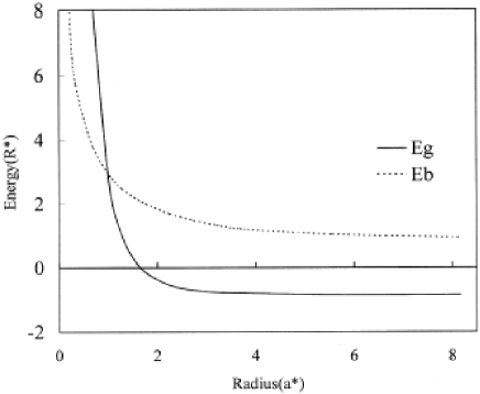
Figure 1: The ground-state energy(solid line) and the binging energy (dotted line) of a hydrogenic impurity located at the axis of a cylindrical wire as a function of the radius of the wire. (Ry* and a* are effective rydberg and the effective Bohr radius.)

Figure 1 shows the ground state energy as a function of the wire radius. The binding energy $E_{b}$ of the hydrogenic impurity is defined as the energy difference between the ground state energy of the cylindrical wire system with and without the impurity, i.e.

$$E_{b}=E_{0}-E_{g}$$ (39)

where $E_{0}$ is the ground state energy of the quantum wire system without the impurity, while $E_{g}$ is the ground state energy of the quantum wire system with the impurity located on the axis of the cylindrical wire. One can see from Fig.1 that the energy of the 1$s$ state becomes negative when the wire radius is larger than 1.65$a^{\ast}$. It means that the confining energy is larger than the Coulomb energy as the wire radius is smaller than 1.65$a^{\ast}$. And one can also note that as the radius of the quantum wire is decreased, the ground state energy increases. As the wire radius $d$ becomes smaller, the electron is pushed toward the axis of the cylindrical wire. This makes the electron get close to the nucleus. As the electron gets close to the nucleus, both the ground state energy and the binding energy increase rapidly. This is because the Coulomb potential, which varies with $\sim\frac{1}{d}$ ($d$ is the wire radius), becomes more negative, while the kinetic energy of the electron, which varies with $\sim\frac{1}{d^{2}}$ (by the uncertainty relation), increases more rapidly. As a result, the ground state energy is increased as the electron gets close to the nucleus. The binding energy defined in Eq. (39) is effectively the negative sign of the of the Coulomb interaction energy between the electron and the nucleus, i.e. $\sim\frac{1}{d}$, therefore, the binding energy of the electron is also increased as the electron gets near to the nucleus.. As a result, the ground state energy is increased as the electron gets close to the nucleus. The binding energy defined in Eq. (39) is effectively the negative sign of the of the Coulomb interaction energy between the electron and the nucleus, i.e. $\sim\frac{1}{d}$, therefore, the binding energy of the electron is also increased as the electron gets near to the nucleus. Our results show that for small wire radius, the binding energies are in good agreement with previous results11 ; 14 . As the radius becomes very large, our result approaches the correct limit 1$R^{\ast}$ while the previous work 14 can only yield a value of 0.22$R^{\ast}$. The large discrepancy of the previous work may be due to the artificial dividing of the variational trial wavefunction into a one-dimensional hydrogen atom and a two-dimensional hydrogen atom and thus forces the creation of an additional node of the wavefunction at z=0. In this work, the trial wavefunction is adopted to be the form of 1D harmonic oscillator wavefunction instead of one dimensional hydrogen atom. This prevents our wavefunction from introducing any additional node at z=0.Figure 2 presents the 2s excited state binding energies as the functions of wire radius. One can note from the figure that as the wire radius increases, the binding energy approaches 0.25$R^{\ast}$ which gives correctly the limiting value of 3D hydrogen atom.

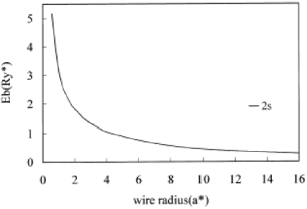
Figure 2: The binding energy of the 2s excited state as a function of the wire radius. (Ry* and a* are effective rydberg and the effective Bohr radius.)

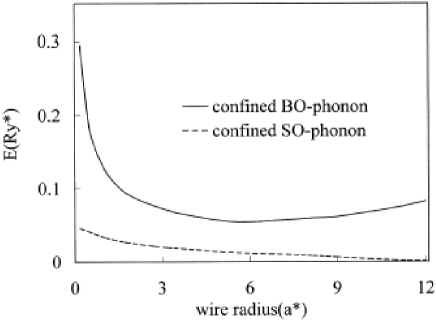
Figure 3: The energies of the wire radius modified by the confined BO and SO phonon. The solid line stands for the BO phonon effect, and the dashed line for the SO phonon effect. (Ry* and a* are effective rydberg and the effective Bohr radius.)

Figure 3 presents the confined BO phonon and SO phonon effect as a function of wire radius. With increasing the wire radius, the magnitude of the confined BO phonon effect decreases from large value and then approaches to the bulk value. When the wire radius is less than 1.5 a*, the polaron effect increases rapidly. One might think as the radius becomes very small, the confined BO phonon effect should approach zero, like the case in quantum well 31 . In fact, similar results were obtained by Oshiro in a spherical quantum dot32 . They found the polaron energy shift is enhanced as the dot radius becomes small. This is due to the fact that the electron becomes complete localized (E_b approaches infinity) in small wire (or dot) radius while the binding energy approaches 4$R^{\ast}$ in small well width. In the case of quantum well, the confined SO phonon effect plays the dominant role for small well width31 . But in quantum wire, the confined SO phonon is less important, just like that in quantum dot system 32 . This is because the surface area of a quantum wire (or quantum dot) decreases with the radius. Thus the number of vibration modes of confined SO phonon becomes fewer.

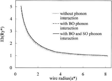
Figure 4: The binding energy with/without phonon effect. The dotted line stands for the binding energy without the phonon effect. The dashed line stands for that only BO phonon effect on the binding energy, and the solid line for both the BO and SO phonons effects on the binding energy. (Ry* and a* are effective rydberg and the effective Bohr radius.)

In Fig.4, three curves are presented. The dotted curve represents the binding energy of the impurity without considering the interactions between the electron and phonon. The dashed curve represents the binding energy of the impurity with only confined BO phonon effect being taken into account. While the solid curve is the binding energy of the impurity including both confined BO phonon and SO phonon effects in the calculation. Comparing to the impurity binding energy, the confined SO phonon is negligible in quantum wire. We then conclude that because of the similarity in geometry, the behavior of the polaron effect on the quantum wire system is like that on the quantum dot system.

IV Conclusion

In this work, analytical solutions for the effects of the electron-phonon interaction on the binding energies of an impurity located inside a quantum wire are obtained by a simple but efficient perturbation-variation method. As the radius becomes very large, the correct limiting value can be obtained. We have also discussed both the confined BO and SO phonon effects. We found the confined BO phonon effect is prominently for a quantum wire with small radius. We also found that the energy corrections of the polaron effects on the impurity binding energies increase rapidly when the wire radius is less than 1.5 a*.

Acknowledgements

This work is supported partially under the grant number NSC 88-2112-M-009-004 by the National Science Council, Taiwan.

References

- (1) R. C. Miller, D. A. Kleinman, and W. T. Tsang, Phys.Rev. B24, 1134 (1981).
- (2) A. B. Fowler, A. Harstein, and R. A.Webb, Phys. Rev. Lett. 48, 196 (1982).
- (3) P. H. Petroff, A. C. Gossard, R. A. Logan, and W. Wiegman, Appl. Phys. Lett. 41, 635 (1985).
- (4) A. S. Plaut et al, Phys. Rev. Lett. 67, 1642 (1991).
- (5) G. Bastard, Phys. Rev. B24, 4714 (1981).
- (6) C. Mailhiot, Y. C. Chang, and T. C. McGill, Phys. Rev. B26, 4449 (1982).
- (7) R. L. Greene and K. K. Bajaj, Solid State Commun. 45, 825 (1983).
- (8) W. M. Liu and J. J. Quinn, Phys. Rev. B35, 2348 (1985).
- (9) J. W. Brown and H. N. Spector, J. Appl. Phys. 59, 1179 (1986).
- (10) G. W. Brynt, Phys. Rev. B29, 6632 (1984); B31, 7812 (1985).
- (11) S. V. Branis, G. Li, and K. K. Bajaj, Phys. Rev. B47, 1316 (1993).
- (12) G. W. Bryant, Phys. Rev. B37, 8763 (1988).
- (13) J. Lee and H. N. Spector, J. Appl. Phys. 54, 3921(1983); 57, 366 (1985).
- (14) D. S. Chuu, C. M. Hsiao and W. N. Mei, Phys. Rev. B46, 3898 (1992).
- (15) H. Sakai, Jpn. J. Appl. Phys. 19, L735 (1980).
- (16) M. H. Degani, and O.Hipólito, Phys. Rev. B33, 4090 (1986).
- (17) B. A. Mason and S. Das Sarma, Phys. Rev. B33, 8379 (1986).
- (18) A. Ercelebi and M. Tomak, Solid State Commun. 54, 883 (1985).
- (19) Z. J. Shen, X. Z. Yuan, G. T. Shen and B. C. Yang, Phys. Rev. B49, 11053 (1994).
- (20) A. Thilagam and J. Singh, Phys. Rev. B49, 13583 (1994).
- (21) A. Ercelebi and U. Özdincer, Solid State Commun. 57, 441 (1986).
- (22) M. H. Degani, and O. Hipólito, Phys. Rev. B35, 4507 (1988).
- (23) D. S. Chuu, W. L. Won and J. H. Pei, Phys. Rev. B49, 14554 (1994).
- (24) R. S. Zheng and M. Matsuura, Phys. Rev. 57, 1749 (1998).
- (25) F. Osorio, M. H. Degani, and O. Hipólito, Phys. Rev. B52, 4662 (1995).
- (26) H. Y. Zhou and S. W. Gu, Solid State Commun. 89, 937 (1994).
- (27) A. Ercelebi and R. T. Senger, Phys. Rev. B53, 11008 (1996).
- (28) T. F. Jiang and D. S. Chuu, Physica B164, 287 (1990) and the References therein.
- (29) W. S. Li and C. Y. Chen, Physica B229, 375 (1997)
- (30) L. D. Landau and S. I. Pekar, Zh.Eksp.Teor.Fiz. 16, 341 (1946).
- (31) R. Zheng, S. Ban, and X. X. Liang, Phys. Rev. B49. 1796 (1994).
- (32) K. Oshiro, K. Akai, and M. Matsuura, Phys. Rev. B58, 7986 (1998).