Noise-induced macroscopic bifurcations in populations of globally coupled maps

Abstract

Populations of globally coupled identical maps subject to additive, independent noise are studied in the regimes of strong coupling. Contrary to each noisy population element, the mean field dynamics undergoes qualitative changes when the noise strength is varied. In the limit of infinite population size, these macroscopic bifurcations can be accounted for by a deterministic system, where the mean-field, having the same dynamics of each uncoupled element, is coupled with other order parameters. Different approximation schemes are proposed for polynomial and exponential functions and their validity discussed for logistic and excitable maps.

Introduction. A fundamental question that arises when physical and biological populations are described by means of mathematical models is how the collective dynamics is qualitatively affected by random fluctuations acting at the microscopic level. While for systems at equilibrium a well established thermodynamic theory exists, for out-of-equilibrium phenomena, such as those typically described by nonlinear dynamical systems, an overall theoretical view is still lacking. In this Letter we will address one aspect of this issue, namely the effect of microscopic noise on the mean-field dynamics of large populations of globally and strongly coupled identical maps.
Systems of globally coupled units are meant to model, among others, Josephson junction arrays Hadley et al. (1988), yeast cells in a continuous-flow, stirred tank reactor Danø et al. (1999) and neural cells Sompolinsky et al. (1991), and provide a mean field description of spatially extended systems with long enough correlation length.
The effect of noise on one dynamical system has been extensively studied, pointing out phenomena such as noise-induced bifurcations, stochastic and coherence resonance (for a review, see Ref. Toral et al. (2001) and references therein). Synchronization phenomena induced by (common or independent) noise have been studied for a system of two coupled dynamical systems Maritan and Banavar (1994); Pikovsky (1994); Neiman et al. (1995); Andrade et al. (2000); Zhou and Kurths (2002); Zhou et al. (2002). In the context of populations, the effect of microscopic noise on the collective dynamics has been recently inquired for continuous-time systems, namely phase models Kurrer and Shulten (1995); Moro and Sánchez (1998); Hong and Choi (2000); Hasegawa , integrate-and-fire neurons Rappel and Karma (1996); Teramae , excitable systems Sosnovtseva et al. (2001); Naundorf et al. , chaotic systems Zanette and Mikhailov (2000); Teramae and Kuramoto (2001). The onset of collective oscillations and the dependence of their frequency from the noise intensity has been mainly addressed. Analogous synchronization phenomena have been detected for stochastic oscillators Nikitin et al. (2001); Naundorf et al. and in spatially extended systems Neiman et al. (1999); Ibañes et al. (2001).
Concerning maps, the relationship between single element and mean field fluctuations close to bifurcations Nichols and Wiesenfeld (1994) and the anomalous scaling of the population moments close to the onset of synchronization Teramae and Kuramoto (2001) have been inquired.
However, the qualitative changes of the macroscopic dynamics under the influence of noise have, at our best knowledge, never been systematically addressed. In particular, the strong coupling regimes could be considered of little interest since one expects the addition of a weak noise term not to greatly alter the mean field behavior. Instead, in the first part of this Letter we give numerical evidence of the fact that noise can qualitatively change the macroscopic dynamics of the system: even if the single map has a noisy temporal series, the mean field displays a low dimensional behaviour which can be different with respect to the uncoupled map dynamics. The phenomenon of noise-induced macroscopic bifurcations will be illustrated for two kinds of maps: logistic maps in the chaotic regime and “excitable maps”. Contrary to noise-induced synchronization, in this case it is the coupling that induces a coherent behavior for low noise intensity. The deterministic trajectory of each dynamical system is blurred out, so that the bifurcations detectable at a macroscopic level are a purely collective effect and cannot be inferred by looking at one or few population elements.

In the second part of the Letter, we explain these phenomena by means of an order parameter expansion, valid for sufficiently large coupling strength and large population size. This provides an approximate description of the mean field dynamics in terms of few effective macroscopic variables, whose deterministic equations of motion account for the macroscopic dynamics of the population and for the bifurcations among different collective regimes. The validity of such approach will be demonstrated on the two aforementioned populations of maps. In particular, for the logistic maps the bifurcation diagram of the mean field will be rescaled to that of a single logistic map.

Noise effect on coherent regimes. Let us consider populations of noisy and globally coupled identical one-dimensional maps. We choose this system because it is sufficiently simple to be analytically treated, and, at the same time, can be considered as a prototype for inquiring new phenomena.
The fact that the mean field can exhibit complex dynamics is well known Kaneko (1989, 1990); Pikovsky and Kurths (1994); ans S. Tsukada (2002) and in particular we will focus on the synchronous regimes appearing for sufficiently strong coupling.
The equation of each population element is defined as follows:

$$x_{j}\mapsto(1-k)\>f(x_{j})+k\>\langle\,{f(x)}\,\rangle+\xi_{j}(t)\qquad j=1,2,\dots N,$$ (1)

where $x_{j}\in\mathbb{R}$ is the state of the j-th population element, $f:\mathbb{R}\rightarrow\mathbb{R}$ is a smooth function defining the uncoupled elements dynamics and $\langle\,{f(x)}\,\rangle:=\sum_{j=1}^{N}\,f(x_{j})/N$ is the average over the population. Every map is subject to a noise $\xi_{j}(t)$, that is determined according to a distribution of assigned moments (in particular, it does not need to be Gaussian). The noise terms are independent and delta correlated, that is:

$$\xi_{i}(t)\xi_{j}(t^{\prime})=\sigma^{2}\,\delta_{i,j}\,\delta_{t,t^{\prime}},$$

where $\sigma^{2}$ is the variance of the noise terms distribution, measuring the intensity of the microscopic noise.
Keeping all the parameter fixed, we will study the asymptotic behaviour of the mean field $X=\langle\,{x}\,\rangle$ of large populations when $\sigma$, that will be from now on our control parameter, is changed.
Figure 1 shows the bifurcation diagram of $X$ in the case of half a million logistic maps in the chaotic regime, together with the phase portrait of an individual element of the population.

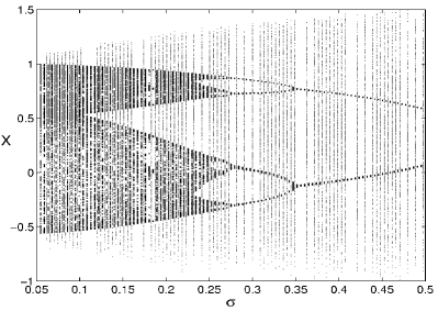
Figure 1: Phase portrait of the mean field $X$ (big dots) of $N=2^{19}$ logistic maps of the form $f(x)=1-a\,x^{2}$ ($a=1.57$, $k=0.7$) (and of one population element $x$ (small dots)) as a function of the noise standard deviation $\sigma$. The noise terms are generated according to a uniform distribution.

When the noise intensity is small, all the elements of the population evolve coherently on a chaotic attractor. In the limit of zero noise, indeed, all the elements are perfectly synchronized and have a common chaotic trajectory (the assumption of strong coupling prevents the formation of clusters). For larger noise intensities, the mean field displays an inverse bifurcation cascade, crossing several periodic windows and undergoing a period-halving scenario. This simplification of the mean field dynamics does not however reflect on the individual elements of the population, whose dynamics is more and more smeared out with the increase of the microscopic noise.
As we will later phrase in more rigorous terms, the fact that the average has a regular behavior is a consequence of the fact that, in the population, a large number of simultaneous realizations of the noise occurs, so that only statistical averages of the microscopic stochastic process are relevant.
As a second example of bifurcations induced by microscopic noise we consider an “excitable map” of the form (for other definitions of “excitable map” see Refs. Hayakawa and Sawada (2000); Toral et al. (2001)):

$$f(x)=(\alpha\,x+\gamma\,x^{3})\>e^{-\beta\,x^{2}}.$$ (2)

The parameters are chosen in a region where the origin is the only fixed point, but, if the system is initiated far enough from it, there is a chaotic transient. The effect of noise on the single map is thus of exciting it over threshold, so that a complex dynamics takes place.

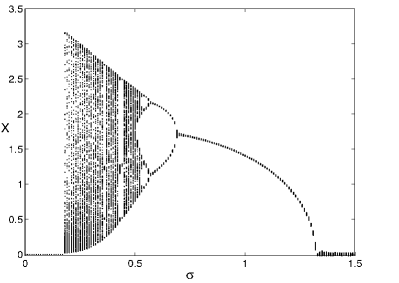
Figure 2: Phase portrait of the mean field $X$ of $N=524288$ excitable maps of Eq. (2) ($\alpha=.4$, $\beta=1$, $\gamma=8$, $k=0.9$) as a function of the noise standard deviation $\sigma$. The noise terms are generated according to a Gaussian distribution.

Correspondingly, the mean field has, for small noise intensity, fluctuations above zero scaling as $\sigma/\sqrt{N}$, up to a critical point, where the mean field starts displaying large amplitude chaotic oscillations (Figure 2). The asymptotic dynamics simplifies for higher values of $\sigma$, the mean field going through a backwards bifurcation cascade up to a steady state. For very large noise values, the fixed point drops again to zero, as a consequence of the fact that the map in Eq. (2) is odd and a strong noise causes the population to spread symmetrically around the mean field.

Order parameter expansion. Let us now address the problem from a mathematical viewpoint, performing a change of variables that allows us to decouple the macroscopic effect of noise from the dynamic “skeleton” furnished by the uncoupled map equation. This is achieved expressing the position of each population element in terms of the mean field and of its displacement from it:

$$x_{j}=X+\epsilon_{j}\hskip 56.9055ptj=1,2,\dots N.$$ (3)

We can now substitute Eq. (3) into the uncoupled element equation and expand it in series around the mean field, thus obtaining:

$$f(x_{j})=f(X)+\sum_{q=1}^{\infty}\>\frac{1}{q!}\>\mathcal{D}^{q}f(X)\>\epsilon_{j}^{q},$$ (4)

where $\mathcal{D}^{q}f$ indicates the $q$-th derivative of the function $f$. The equation for the mean field can now be obtained directly from its definition, thus getting:

$$X\mapsto\langle\,{f(x)}\,\rangle=f(X)+\sum_{q=1}^{\infty}\>\frac{1}{q!}\>\mathcal{D}^{q}f(X)\>\langle\,{\epsilon^{q}}\,\rangle$$ (5)

We have at this point discarded the term $\langle\,{\xi}\,\rangle$ that vanishes in the limit of infinite population size and, otherwise, plays the role of a macroscopic noise acting on the mean field and scaling as $1/\sqrt{N}$, according to the law of large numbers.
Let us now define a set of new order parameters:

$$\Omega_{q}:=\langle\,{\epsilon^{q}}\,\rangle\hskip 56.9055ptq\in\mathbb{N},$$ (6)

and compute their evolution by making use of:

$$\epsilon_{j}\mapsto(1-k)\>\sum_{p=1}^{\infty}\>\frac{1}{p!}\>\mathcal{D}^{p}f(X)\>\left(\epsilon_{j}^{p}-\Omega_{p}\right)+\xi_{j}$$

and of the fact that, being the positions and the noise uncorrelated variables, in the limit $N\to\infty$ holds: $\langle\,{h(X,\epsilon)\>\xi^{q}}\,\rangle=\langle\,{h(X,\epsilon)}\,\rangle\>\langle\,{\xi^{q}}\,\rangle.$ From simple algebra thus follows:

$$\Omega_{q}\mapsto m_{q}+\sum_{i=1}^{q}\binom{q}{i}(1-k)^{i}\>m_{q-i}$$ (7)

$$\qquad\langle\,{\left[\sum_{p=1}^{\infty}\>\frac{1}{p!}\>\mathcal{D}^{p}f(X)\>\left(\epsilon^{p}-\Omega_{p}\right)\right]^{i}}\,\rangle,$$

where $m_{q}=\langle\,{\xi^{q}}\,\rangle$ is the $q$-th moment of the noise distribution.

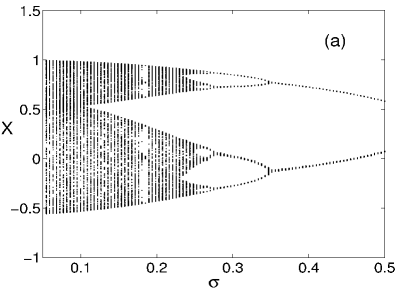
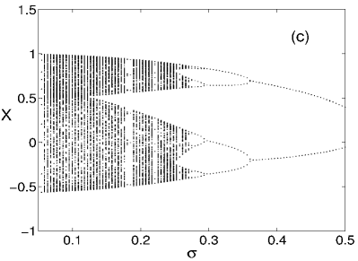
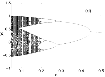
Figure 3: Phase portrait, as a function of the (uniformly distributed) noise standard deviation $\sigma$, of a) the mean field of a population ($N=524288$) of logistic maps of the form $f(x)=1-a\,x^{2}$ ($a=1.57$) for high coupling ($k=0.9$); b) the mean field of the same population for weaker coupling ($k=0.7$); c) the zeroth-order expansion Eq. (8); the second order expansion Eq. (Noise-induced macroscopic bifurcations in populations of globally coupled maps). For lower coupling values, the qualitative agreement improves if further order parameters are taken into account.

As a first approximation, valid for high coupling strength, the mean field dynamics can be described by a scalar equation:

$$X\mapsto f(X)+\sum_{q=1}^{\infty}\>\frac{1}{q!}\>\mathcal{D}^{q}f(X)\>m_{q}$$ (8)

which is obtained by Eqs. (5) and (7) in the limit $k\to 1$.
The two left-hand pictures of Figure 3 show the mean field dynamics for the population of logistic maps under high coupling ($k=0.9$, top) and for the effective mean field dynamics Eq. (8) (bottom), that in this case takes the simple form:

$$X\mapsto 1-a\>\sigma^{2}-a\>X^{2}.$$ (9)

This equation provides a rescaling of the average population dynamics to that of a single logistic map of the form $b+a\>X^{2}$.
A more difficult case to analyse is that of the excitable maps, since in this case the sum in Eq. (8) contains an infinite number of terms. Any finite truncation thus introduces a further approximation, whose validity holds for sufficiently weak noise. Figure 4 reports the mean field bifurcation diagram for the population (left) and for the sixth-order truncation of Eq. (8) (right), that is able to describe the onset of the collective chaotic oscillations up to the first periodic windows.

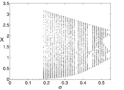
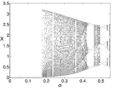
Figure 4: Phase portrait as a function of the (normally distributed) noise standard deviation $\sigma$ of the mean field of a population ($N=2^{1}9$) of excitable maps described by Eq. (2) ($\alpha=6$, $\beta=1$, $\gamma=8$) for $k=0.9$ (top left) and for Eq. (8) truncated at the sixth order. Lower order truncations lead to less accurate approximations (not shown).

It is worth noticing that the terms of high order in the series of Eq. (8) are small for low noise intensity, so being the noise distribution moments. Therefore, increasing the noise variance from zero causes the nonlinearities of the uncoupled map to become progressively important in the mean field dynamics description. In general, we can see that Eq. (8) accounts for the influence of the noise distribution features (described by its moments) on the dynamics of an uncoupled element. If this is a polynomial, the $q$-th moment will affect the coefficients of the terms of order less than $q$. It is however important to stress that no requirements have been made on the specific shape of the noise distribution, so that distributions having the same low-order moments have similar macroscopic effects for weak noise.

Let us now consider the case of lower coupling and include in the effective description also the terms in $(1-k)^{2}$ (those in $(1-k)$ cancel out for symmetrical noise distributions, like those considered so far):

$$X\mapsto f(X)+\sum_{q=1}^{\infty}\>\frac{1}{q!}\>\mathcal{D}^{q}f(X)\>\Omega_{q}$$

$$\Omega_{q}\mapsto m_{q}+\frac{q(q-1)}{2}\>(1-k)^{2}\>m_{q-2}$$

$$\qquad\sum_{p=1}^{\infty}\frac{1}{p^{2}!}\>\left[\mathcal{D}^{p}\,f(X)\right]^{2}\>\left(\Omega_{2p}-\Omega_{p}^{2}\right)$$

If $f$ is a polynomial of order $n$, the reduced system Eq. (Noise-induced macroscopic bifurcations in populations of globally coupled maps) is a closed system of $2n+1$ variables, which thus determine the dimensionality of the mean field dynamics. Again, when $f$ is not a polynomial, any truncation of Eq. (Noise-induced macroscopic bifurcations in populations of globally coupled maps) introduces errors which become bigger when the noise intensity increases. Nevertheless, the moments of high order become negligible when $\sigma$ is small and the mean field dynamics can still be described in the weak noise regimes.
Going back to the previously considered population of logistic maps, we lower the coupling strength. Equation (Noise-induced macroscopic bifurcations in populations of globally coupled maps) takes now the following form:

$$X\mapsto 1-a\,X^{2}-a\>\Omega_{2}$$

$$\Omega_{2}\mapsto \sigma^{2}+(1-k)^{2}\,a^{2}\left(4\,X^{2}\,\Omega_{2}-\Omega_{2}^{2}+\Omega_{4}\right)$$ (11)

$$\Omega_{4}\mapsto m_{4}+6(1-k)^{2}a^{2}\sigma^{2}\left(4X^{2}\Omega_{2}-\Omega_{2}^{2}+\Omega_{4}\right)$$

The two right-hand images of Figure 3 compare the mean field dynamics for $k=0.7$ (top) with that of the second order approximation Eq. (Noise-induced macroscopic bifurcations in populations of globally coupled maps) (bottom). the mean field dynamics can be directly compared with the zeroth-order approximation (bottom left of the same figure), that is independent of $k$. It is evident that the accordance with the population bifurcation scenario is improved when more order parameters are introduced in the description. In particular, Eq. (Noise-induced macroscopic bifurcations in populations of globally coupled maps) reproduces the shift of the period-doubling cascade toward lower values of the noise intensity, taking place when the coupling is weakened.

Conclusions. In this Letter we have discussed the phenomenon of macroscopic bifurcations induced by microscopic additive noise in large populations of globally and strongly coupled maps. We have shown that the macroscopic dynamics changes with the noise intensity and that in the case of high coupling the macroscopic bifurcations can be reproduced by a low-dimensional map, where the mean field is coupled to some additional order parameters. This order parameter reduction accounts for the effects of noise on the dynamical “skeleton” given by the uncoupled element equation. The proposed method holds for any smooth map and is largely independent from the specific characteristics of the noise distribution, allowing to understand how the noise moments interact with the nonlinearities of the uncoupled map equation. As examples of application, we have considered logistic maps in the chaotic regime and excitable maps, and we have addressed the validity of different approximation schemes.
Although populations of scalar maps have been considered in order to simplify both the analytical and the numerical work, studies on continuous-time systems (in particular, Refs. Kurrer and Shulten (1995); Hong and Choi (2000) together with our preliminary results indicate that microscopic noise might have a similar effect on strongly coupled continuous time systems, inducing macroscopic bifurcations of the mean field. The method presented here could be combined with the order parameter expansion proposed in Ref. Monte et al. for investigating the different roles of microscopic noise and intrinsic parameter diversity on populations of dynamical systems.

References

- Hadley et al. (1988) P. Hadley, M. R. Beasley, and K. Wiesenfeld, Phys. Rev. B 38, 8712 (1988).
- Danø et al. (1999) S. Danø, P. G. Sørensen, and F. Hynne, Nature 402, 320 (1999).
- Sompolinsky et al. (1991) H. Sompolinsky, D. Golomb, and D. Kleinfeld, Phys. Rev. A 43, 6990 (1991).
- Toral et al. (2001) R. Toral, C. R. Mirasso, E. Hernández-García, and O. Piro, Chaos 11, 665 (2001).
- Maritan and Banavar (1994) A. Maritan and J. Banavar, Phys. Rev. Lett. 72, 1451 (1994).
- Pikovsky (1994) A. Pikovsky, Phys. Rev. Lett. 73, 2931 (1994).
- Neiman et al. (1995) A. Neiman, U. Feudel, and J. Kurths, J. Phys. A 28, 2471/2480 (1995).
- Andrade et al. (2000) V. Andrade, R. L. Davidchack, and Y. Lay, Phys.Rev. E 61, 3230 (2000).
- Zhou and Kurths (2002) C. Zhou and J. Kurths, Phys. Rev. Lett. 88, 230602 (2002).
- Zhou et al. (2002) C. Zhou, J. Kurths, I. Kiss, and J. Hudson, Phys. Rev. Lett. 89, 014101 (2002).
- Kurrer and Shulten (1995) C. Kurrer and K. Shulten, Phys. Rev. E 51, 6213 (1995).
- Moro and Sánchez (1998) E. Moro and A. Sánchez, Europhys. Lett. 44, 409 (1998).
- Hong and Choi (2000) H. Hong and M. Choi, Phys. Rev. E 62, 6462 (2000).
- (14) H. Hasegawa, cond-mat/0210473.
- Rappel and Karma (1996) W. Rappel and A. Karma, Phys. Rev. Lett. 77, 3256 (1996).
- (16) J. Teramae, cond-mat/0210048.
- Sosnovtseva et al. (2001) O. Sosnovtseva, A. Fomin, D. Postnov, and V. Anishchenko, Phys. Rev. E 64, 026204 (2001).
- (18) B. Naundorf, T. Prager, and L. Schimansky-Geir, cond-mat/02110111.
- Zanette and Mikhailov (2000) D. Zanette and A. S. Mikhailov, Phys. Rev. E 62, R7571 (2000).
- Teramae and Kuramoto (2001) J. Teramae and Y. Kuramoto, Phys. Rev. E 63, 036210 (2001).
- Nikitin et al. (2001) A. Nikitin, Z. Neda, and T. Vicsek, Phys. Rev. Lett. 87, 024101 (2001).
- Neiman et al. (1999) A. Neiman, L. Schimansky-Geier, A. Cornell-Bell, and F. Moss, Phys. Rev. Lett. 83, 4896 (1999).
- Ibañes et al. (2001) M. Ibañes, J. García-Ojalvo, R. Toral, and J. Sancho, Phys. Rev. Lett. 87, 020601 (2001).
- Nichols and Wiesenfeld (1994) S. Nichols and K. Wiesenfeld, Phys. Rev. E 49, 1865 (1994).
- Kaneko (1989) K. Kaneko, Phys. Rev. Lett. 63, 219 (1989).
- Kaneko (1990) K. Kaneko, Physica D 41, 137 (1990).
- Pikovsky and Kurths (1994) A. Pikovsky and J. Kurths, Phys. Rev. Lett. 72, 1644 (1994).
- ans S. Tsukada (2002) T. S. ans S. Tsukada, Physica D 168-169, 126 (2002).
- Hayakawa and Sawada (2000) Y. Hayakawa and Y. Sawada, Phys. Rev. E 61, 5091 (2000).
- (30) S. D. Monte, F. d’Ovidio, and E. Mosekilde, Phys. Rev. Lett., to appear.