Three-dimensional lattice-Boltzmann simulations of critical spinodal decomposition in binary immiscible fluids

Abstract

We use a modified Shan-Chen, noiseless lattice-BGK model for binary immiscible, incompressible, athermal fluids in three dimensions to simulate the coarsening of domains following a deep quench below the spinodal point from a symmetric and homogeneous mixture into a two-phase configuration. The model is derivable from a continuous-time Boltzmann-BGK equation in the presence of an intercomponent body force. We find the average domain size growing with time as $t^{\gamma}$, where $\gamma$ increases in the range $0.545\pm 0.014<\gamma<0.717\pm 0.002$, consistent with a crossover between diffusive $t^{1/3}$ and hydrodynamic viscous, $t^{1.0}$, behaviour. We find good collapse onto a single scaling function, yet the domain growth exponents differ from others’ works’ for similar values of the unique characteristic length $L_{0}$ and time $T_{0}$ that can be constructed out of the fluid’s parameters. This rebuts claims of universality for the dynamical scaling hypothesis. For $\mathrm{Re}=2.7$ and small wavenumbers, $q$, we also find a $q^{2}\leftrightarrow q^{4}$ crossover in the scaled structure function, which disappears when the dynamical scaling reasonably improves at later stages ($\mathrm{Re}=37$). This excludes noise as the cause for a $q^{2}$ behaviour, as analytically derived from Yeung and proposed by Appert et al. and Love et al. on the basis of their lattice-gas simulations. We also observe exponential temporal growth of the structure function during the initial stages of the dynamics and for wavenumbers less than a threshold value, in accordance with the diffusive Cahn-Hilliard Model B. However, this exponential growth is also present in regimes proscribed by that model. There is no evidence that regions of parameter space for which the scheme is numerically stable become unstable as the simulations proceed, in agreement with finite-difference relaxational models and in contradistinction with an unconditionally unstable lattice-BGK free-energy model previously reported. Those numerical instabilities that do arise in this model are the result of large intercomponent forces which turn the equilibrium distribution negative.

1 Introduction

Homogeneous binary fluid mixtures phase segregate into two phases with different compositions when quenched into thermodynamically unstable regions of their phase diagram, a process also called spinodal decomposition. This is achieved by lowering the temperature well below the so called spinodal temperature. For incompressible, 50:50 mixtures, also called critical or symmetric mixtures, these phases form interconnected domains which at late times produce a bicontinuous structure with sharp, well developed interfaces. For asymmetric mixtures (phases with different densities) there is a phase transition at early times from an interpenetrating structure termed as “bicontinuous” to the so-called “droplet phase”, which in turn undergoes subsequent coarsening via coalescence [1]. The composition of a binary immiscible fluid is one of the variables affecting its dynamics. Fields where spinodal decomposition is of industrial relevance comprise the metallurgical, oil, food, paints and coatings industries. Polymer blends and gels immersed in a solvent are also potentially important applications where phase separation occurs and needs to be controlled [17, 18].

Spinodal decomposition has been extensively studied by experimental [2], analytical [3, 4], and numerical [5, 6, 7, 8, 9, 10, 11, 12, 56, 28] approaches. The fact that it entails a variety of mechanisms that can act concurrently and at different length and time scales has made it a testbed for complex fluid simulation methods. Among the latter are hydrodynamic lattice gases [46], the lattice Boltzmann equation [13], and dissipative particle dynamics [47].

Despite all the interest attracted by the subject, how the mechanisms responsible for domain separation act remains on unsettled grounds. In particular, the dynamics of the late time, true asymptotic growth is unclear. Also, the dynamical scale invariance hypothesis (to be explained later on in this paper), which is treated almost as canonical by analytical and numerical approaches to solving the continuum, local-thermodynamic Cahn-Hilliard equations, has experimentally been proven to fail at least under certain conditions [29].

Numerical studies on spinodal decomposition include methods at the macroscopic scale, based on the numerical solution of either the Navier-Stokes [50, 53] or the Cahn-Hilliard equations [51, 5, 55], the mesoscopic scale, where lattice-Boltzmann (LB) methods [14, 15], lattice gases [8, 7], dissipative particle dynamics [48], and Ising [49] approaches are examples, and the microscopic scale, with classical molecular dynamics [12].

Fluid dynamical methods in the mesoscopic scale came to light as a way to grasp the relevant thermohydrodynamical behaviour with as little computational effort as possible. This is achieved by evolving a microworld in which the usual vast number of molecular degrees of freedom and characterisation have been drastically reduced, based on the fact that, away enough from critical points, a fluid’s macrostate is pretty much insensitive to many of its microscopic properties. Some regard the Cahn-Hilliard equations to be within the mesoscopic scale. They derive from the van der Waals’ formulation of quasilocal thermodynamics [37], extended by Cahn and Hilliard [51], and aim at solving a Langevin-like diffusion equation for the conserved order parameter. This equation involves a chemical potential derived from a phenomenological, Ginzburg-Landau expansion for the free energy, and leads to phase segregation if the temperature is below a critical value. The scheme commonly used for the study of phase segregation in immiscible fluids is termed Cahn-Hilliard Model H [33]; hydrodynamics is included by introducing mass currents, which couple the diffusion equation with the Navier-Stokes equation. Thermal effects are sometimes included in the dynamics by the addition of a noise term satisfying a fluctuation-dissipation theorem.

Cahn-Hilliard equations have been applied to model the segregation dynamics of deep and sudden thermal quenches of fluid mixtures. Such quenches are usually chosen to be sudden to avoid thermal noise effects and set up an initial condition that quickly leads to a state of steep domain walls and where diffusion is negligible compared with hydrodynamic effects, thus leaving the conditions that the dynamical scaling hypothesis requires. However, local-equilibrium cannot be guaranteed for a mixture undergoing a sudden quench, which puts the existence of a free energy and the equilibrium states modelled by it on rather shaky grounds.

The lattice-Boltzmann method we use in this work is the Shan-Chen lattice-BGK scheme for binary immiscible and incompressible fluid flow [14]. The equilibrium state for each pure fluid is chosen to be a local isothermal Maxwellian, and Shan and Chen’s contribution to the lattice-BGK scheme comes through the phase separation prescription. This is incorporated via intercomponent repulsive mean-field forces between elements of fluids (meant to be at a mesoscopic scale) which alter the local equilibrium, and not through a local equilibrium reproducing a chemical potential derived from a free-energy functional. The Shan-Chen method has been used by Martys and Douglas [34] to qualitatively simulate spinodal decomposition for critical and off-critical quenches in 3D. There have been recent quantitative studies in 2D using this method for critical spinodal decomposition [22, 30]. An early study on critical 2D and 3D spinodal decomposition was put forward by Alexander et al. [35] using the lattice-Boltzmann method proposed by Gunstensen et al [36].

Lattice-BGK methods based on a Ginzburg-Landau free-energy functional [15] achieve multiphase behaviour by using two separate distribution functions: one for the mass density and one for the order parameter, this being defined as the difference between the phases’ densities. Higher-order velocity moments of these distributions are imposed to coincide with thermomechanical quantities obtained from the free energy. The term “top-down” is used in the literature to address this type of approach, whereas we shall use “bottom-up” in the remainder to signify fully mesoscopic methods. Some criticisms of top-down approaches [59] include their frequent lack of Galilean invariance (although Inamuro [38] presented a model that does exhibit this property), and their phenomenological character. Studies of spinodal decomposition using these methods are described in the works of Wagner et al. [10, 16], Kendon et al. [9], and Cates et al. [25].

Numerical instabilities are a great cause for concern in lattice-Boltzmann methods, a study of which will be addressed for the lattice-BGK method we employ in this work. Their sources are two-fold: (a) the finite-difference, discrete-velocity scheme used to solve the BGK-Boltzmann equation prevents the existence of an H-theorem, and (b) the approximations used for the equilibrium distribution do not guarantee its positivity, and hence that of the nonequilibrium distribution. Linear stability analyses have been applied to the lattice-BGK model by Sterling [39], and in more detail by Lallemand and Luo [40] comparing a lattice-BGK model to a generalised LB model with a different relaxation time for each physical flux. Qian et al. [41] gave conditions for the Mach number and the shear viscosity such that the lattice-BGK scheme produces positive mass densities. New approaches to unconditionally stable lattice-Boltzmann models have recently appeared too [42, 43, 44, 45]. They prove the existence of functionals satisfying an H-theorem.

Our objective in this work is to present a bottom-up lattice-BGK method for the study of scaling laws in the spinodal decomposition of critical fluid mixtures in three dimensions. This method has certain advantages over lattice-BGK methods based on a free-energy functional, namely, a smaller number of free parameters to tune, Galilean invariance guaranteed, and a simpler equilibrium distribution. Moreover, it refuses to inject macroscopic information into the mesoscopic dynamics as the top-down methods do, on the grounds that for lattice-BGK methods there is no H-theorem available that guarantees an unconditional approach to a given equilibrium. Indeed, in the context of general complex fluid applications, an expression for the free energy itself may be unknown, and/or its validity be questioned for regimes far enough from local equilibrium, making a top down approach not even viable.

The remainder of the paper is structured as follows. In Section 2 we discuss the dynamical scaling hypothesis, which asserts that after the quench all length scales in the mixture share the same growth law with time. The modified Shan-Chen model we use is explained in Section 3; Section 4 introduces the method we use to measure surface tension, while in Section 5 we describe the simulations performed and the growth laws and scaling functions drawn from them which allow to test the validity of the dynamical scaling hypothesis. Finally, we present our Conclusions in Section 7.

2 Spinodal decomposition

After domain walls have achieved their thinnest configuration via diffusion, the time evolution of the bicontinuous structure that is produced in the phase segregation process that symmetric mixtures undergo presents geometrical self-similarity to the initial stages of such a process when the structure is zoomed in at increasing magnification. This leads us to the dynamical scaling hypothesis, which states that at late times, when diffusive effects have died out, there is a unique characteristic length scale $L$ which grows with time such that the geometrical structure of domains is (in a statistical sense) independent of time when lengths are scaled by $L$ [19]. This amounts to saying that all length scales have the same time evolution. Such a characteristic length scale must be universal for all fluids with the same shear viscosity, $\eta$, density, $\rho$, and surface tension $\sigma$, provided that no mechanisms are involved in their late stage growth other than viscous dissipation, fluid inertia and capillary forces, respectively. This is so because, as we shall see later on, only one length scale can be constructed out of the fluid’s parameters $\eta$, $\rho$, and $\sigma$, these being the only ones present in a hydrodynamic description of the mixture via the Navier-Stokes equations.

The characteristic length scale is usually measured by looking at the first zero crossing of the equal-time pair-correlation function of the order parameter fluctuations [17],

$$C({\mathbf{r}},T)\equiv\langle\phi^{\prime}(\mathbf{x+r},T)\phi^{\prime}({\mathbf{x}},T)\rangle\,,$$ (1)

where, on the lattice, $\langle\rangle\equiv\sum_{\mathbf{x}}\varsigma/V$, $V$ is the spatial volume, $\varsigma$ is the volume of the lattice’s unit cell (hence $V/\varsigma$ is the number of nodes in the lattice), $T$ is the time parameter in time steps, ${\mathbf{r}}$ and ${\mathbf{x}}$ are spatial vectors, and $\phi^{\prime}\equiv\phi-\langle\phi\rangle$ are the order parameter fluctuations, where $\phi({\mathbf{x}})\equiv\rho^{\mathrm{R}}({\mathbf{x}})-\rho^{\mathrm{B}}({\mathbf{x}})$ is the order parameter for our binary fluid (say, a mixture of red (R) and blue (B) phases). The units of $C({\mathbf{r}},T)$ are squared mass density. In the remainder, “lattice units” will mean unity for the mass, length, and time units, respectively, in an arbitrary unit system. The Fourier transform of $C({\mathbf{r}},T)$, called the structure function, is

$$S({\mathbf{k}},T)=\frac{\varsigma}{V}\Big{|}\phi_{\mathbf{k}}^{\prime}(T)\Big{|}^{2}\,.$$ (2)

The units for the structure function are the same as those for the correlation function, and $\phi_{\mathbf{k}}^{\prime}$ is the Fourier transform of the fluctuations. Function (2) is volume-normalised, and gives no power spectrum for infinite lengths, i.e.

$$\frac{\varsigma^{\prime}}{V^{\prime}}\sum_{\mathbf{k}}S({\mathbf{k}},T)=1\,,\qquad S({\mathbf{k}=0},T)=0.$$

where $\varsigma^{\prime}$ is the unit cell volume in reciprocal space, and $V^{\prime}=(2\pi/L)^{3}V/\varsigma=(2\pi)^{3}/\varsigma$ is the reciprocal space volume; in fact, $\varsigma^{\prime}/V^{\prime}=\varsigma/V$. Although Eqs. (1) and (2) are numerically equivalent, the intensity of X-ray and neutron scattering is directly proportional to the structure function, which is hence easily measurable; it is thus this quantity that we prefer to use to measure the system’s characteristic length scales.

We define the (time-dependent) characteristic size $L$ of the domains as

$$L(T)\equiv\frac{2\pi}{k_{1}(T)}\,,$$ (3)

in lattice units, where $k_{1}(T)$ is the first moment (mean),

$$k_{1}(T)\equiv\frac{\sum_{k}kS(k,T)}{\sum_{k}S(k,T)}\,,$$ (4)

of the spherically averaged structure function $S(k,T)$, defined by

$$S(k,T)\equiv\frac{\sum_{\mathbf{\hat{k}}}S({\mathbf{k}},T)}{\sum_{{\mathbf{\hat{k}}}}1}\,,$$ (5)

where ${\mathbf{\hat{k}}}$ indicates the set of wave vectors contained in a spherical shell of thickness one (in reciprocal-space lattice units) centered around ${\mathbf{k}}$, i.e. such that $n-\frac{1}{2}\leq\frac{V^{1/3}}{2\pi}k\leq n+\frac{1}{2}$, $n$ being an integer. $k$ is the modulus of ${\mathbf{k}}$ which is smaller than the Nyquist critical frequency $k_{c}=\pi$ to prevent aliasing. In the limit of short distances and large momenta, scaling arguments lead [19] to the relation

$$S({\mathbf{k}},T)\sim\frac{1}{Lk^{D+1}}$$ (6)

valid for $kL\gg 1$, also known as Porod’s law, where $D$ is the spatial dimension. Short distances here means $\xi\ll r\ll L$, where $\xi$ is the interface thickness.

Other measures have also been used for the system’s characteristic length scale, namely, the position of the structure function’s maximum, and the structure function’s second moment, $k_{2}$ [17]. We chose to use the first moment $k_{1}$ as it is the simplest quantity among the aforementioned. Appert et al. [54] found that the structure function’s maximum’s wavenumber provided a length evolving similarly, although in a noisier fashion, to that derived from the first moment.

Mathematically, the dynamical scaling hypothesis can be written as

$$C({\mathbf{r}},T)=f(r/L)\,,$$ (7)

or

$$S({\mathbf{k}},T)=L^{D}g(kL)\,,$$ (8)

where $L=L(T)$ is a function of time, and $g$ is the Fourier transform of $f$, both of which are the same for any late time slice.

Using methods introduced by Kendon et al. [9], there are unique length and time units that can be defined from the fluid’s density, shear viscosity and surface tension, $\rho$, $\eta$, and $\sigma$, respectively, as follows:

$$L_{0}\equiv\frac{\eta^{2}}{\rho\sigma}\, \qquad T_{0}\equiv\frac{\eta^{3}}{\rho\sigma^{2}}\,.$$ , (9)

We can think of these as a wavelength and a period associated with the system’s fluctuations, respectively, although they do not necessarily have to refer to actual fluctuation averages. We can define the dimensionless variables:

$$l\equiv L/L_{0}\,,\qquad t\equiv(T-T_{\mathrm{int}})/T_{0}\,,$$ (10)

which serve to express the universal character of the dynamical scaling hypothesis. Parameter $T_{\mathrm{int}}$ is an offset that allows one to account for early time diffusional transients and lattice effects. Due to the finite resolution of the lattice the initial condition is not an infinitely fine-grained thorough mixture ($\phi=0$) but there is a non-negligible domain size measured at time $T=0$. We have then to specify a time origin prior to $T=0$, corresponding to a fictitious zero domain size.

For a critical binary immiscible mixture in three dimensions, scaling arguments applied to the terms of the Cahn-Hilliard Model-H equations show that Eq. (7) holds in the asymptotic limit [19], or, equivalently, that

$$l\propto t^{\gamma}\,,$$ (11)

where $\gamma=1$ and $\gamma=2/3$ for the cases when hydrodynamic viscosity and inertia dominate the dynamics, respectively. From the Cahn-Hilliard Model B, which is a Langevin diffusion equation without noise conserving the order parameter [33], an exponent of $\gamma=1/3$ is derived, identical to that obtained from the Lifshitz-Slyozov theory for the growth of a minority phase whose volume fraction is negligible, and is expected to appear at diffusive stages, before hydrodynamics kicks in. Scaling theories do not give any prediction for the crossovers’ positions in time other than that they are “of order unity” [26].

Using a free-energy based, lattice-BGK method, Cates et al. [25] reached the viscous regime ($l\propto t$) for $L_{0}\approx 5.9$ and $\textrm{Re}<0.1$, and the inertial regime ($l\propto t^{2/3}$) for $L_{0}\approx 0.0003$ and $\textrm{Re}<350$. The Reynolds number is defined in this domain-coarsening context as

$$\textrm{Re}\equiv\frac{L}{\nu}\frac{\mathrm{d}L}{\mathrm{d{T}}}=l\dot{l}\,.$$ (12)

where $\nu$ is the kinematic viscosity of the fluid mixture, as defined in the next section, and $\dot{l}$ is the time derivative $\mathrm{d}l/\mathrm{d}t$.

There is also experimental [29] and 2D simulation [10] evidence of breakdown of scale invariance in symmetric binary immiscible quenches. In those experiments, the breakdown of scale invariance occurs [29] for symmetric binary mixtures in confined geometries under the influence of wetting, and a universality has been reported to hold. The process consists of a hydrodynamic coarsening occurring faster than mass diffusion, leaving the system with macroscopic domains whose concentrations are near to but not at the coexisting equilibrium ones. Metastability or instability of the domains then causes a secondary phase separation to kick in via diffusion. Scale invariance and self-similarity have also been recently found to break down for viscoelastic binary fluid mixtures [31]. Finally, there is simulation evidence of breakdown of scale invariance coming from free-energy based, lattice-BGK simulations in 2D. The rationale for this is the coexistence of competing mechanisms at all times in the mixture: diffusion, hydrodynamic modes, and surface tension, giving rise to length scales with different growth exponents [10].

3 Our lattice-Boltzmann model

Initially introduced as a coarse grained version of the lattice-gas automaton method for fluid flow simulation, the lattice-Boltzmann model can also be interpreted as a finite difference solver for the Bhatnagar-Gross-Krook (BGK) approximation to the Boltzmann transport equation [13]. From lattice gases it inherits a particulate, mesoscopic character, as their particles can be assimilated to any physical size which is negligible at a hydrodynamic scale; moreover, unlike lattice-gas automata, no fluctuations are present within the scheme [32]. From the simplicity of the Boltzmann-BGK collision term the LB method gains algorithmic efficiency in simulating fluid flow over solving the incompressible Navier-Stokes equations. When extended to multiphase flows, these features are especially valuable in looking at the complicated domain interfaces that arise in the coarsening of binary mixtures.

The method we use is a modification of the multicomponent, immiscible fluid LB scheme of Shan and Chen [14], which will be explained in detail in Subsection 3.2. The Shan-Chen LB model employs an expansion in Mach number of a Maxwellian equilibrium distribution. Phase-segregating interactions are introduced by means of a self-consistently generated mean-field force between particles. The inclusion of this force gives rise to a non-ideal gas equation of state through the Navier-Stokes equation, which is reproduced via the usual multiscale Chapman-Enskog [20] or moment (Grad) [21] expansion of the distribution function. No thermohydrodynamic behaviour is imposed on the equilibrium distribution, as aforementioned free-energy based, lattice-BGK methods do [15], partly because none of the lattice-Boltzmann implementations reported in the literature so far exhibit an H-theorem ensuring the existence of an asymptote towards a prescribed equilibrium, and partly because a purely mesoscopic, mean-field approach is preferred here. The coefficients of the equilibrium distribution expansion are determined by the conservation of mass and momentum, the property that Galilean invariance holds, and an isotropic pressure tensor.

In this work we employ a pseudo four-dimensional lattice, which is the projection onto 3D of the D4Q24 face-centered hypercubic (FCHC), single-speed lattice, where the notation implies the spatial dimension (4) and the number of vectors linking a site to its nearest neighbours (24). The FCHC lattice guarantees isotropic behaviour for the macrosopic momentum balance equation [24].

In the following subsections we introduce our modified Shan-Chen model, first by looking at a non-interacting mixture of gases, and second including the mean-field force term which gives rise to a non-ideal gas equation of state. Then, we modify the collision term such that the Shan-Chen scheme is consistent with that derived from a Boltzmann-BGK equation in the presence of a force.

3.1 Mixture of ideal gases

The finite-difference, finite-velocity fully-Lagrangian [39] scheme for the numerical solution of the multicomponent Boltzmann equation,

$$n_{k}^{\alpha}(\mathbf{x+c}_{k},t+1)-n_{k}^{\alpha}({\mathbf{x}},t)=\Omega_{k}^{\alpha}\,,$$ (13)

governs the time evolution of the $k$th velocity’s particle number density $n_{k}^{\alpha}$ for the fluid species $\alpha$ in a non-interacting mixture of gases. The lattice-BGK collision term is

$$\Omega_{k}^{\alpha}({\mathbf{x}},t)\equiv-\frac{n_{k}^{\alpha}({\mathbf{x}},t)-n_{k}^{\alpha(\mathrm{eq})}({\mathbf{x}},t)}{\tau^{\alpha}}\,,$$ (14)

where the time increment and lattice spacing are both unity, ${\mathbf{c}}_{k}$ is one of the 24 discrete velocity vectors plus one null velocity, ${\mathbf{x}}$ is a point of the underlying Bravais lattice, and $\alpha=\mathrm{R},\mathrm{B}$ (e.g. oil (R) or water (B)). The parameter $\tau^{\alpha}$ defines a single relaxation rate towards equilibrium for component $\alpha$. The function $n_{k}^{\alpha(\mathrm{eq})}({\mathbf{x}},t)$ is the discretisation of a third-order expansion in Mach number of a local Maxwellian [23],

$$n_{k}^{\alpha(\mathrm{eq})}({\mathbf{x}},t)=\omega_{k}\,n^{\alpha}({\mathbf{x}},t)\Big{[}1+\frac{1}{c_{s}^{2}}{\mathbf{c}}_{k}\cdot{{\mathbf{u}}}+\frac{1}{2c_{s}^{4}}({\mathbf{c}}_{k}\cdot{{\mathbf{u}}})^{2}-\frac{1}{2c_{s}^{2}}u^{2}+\frac{1}{6c_{s}^{6}}({\mathbf{c}}_{k}\cdot{{\mathbf{u}}})^{3}-\frac{1}{2c_{s}^{4}}u^{2}({\mathbf{c}}_{k}\cdot{{\mathbf{u}}})\Big{]}\,,$$ (15)

where $\omega_{k}$ are the coefficients resulting from the velocity space discretisation, and $c_{s}$ is the speed of sound, both of which are determined by the choice of the lattice. For the projected-D4Q24 lattice we use, the speed of sound is $c_{s}=1/\sqrt{3}$, and $\omega_{k}=1/3$ for the speed $c_{k}=0$ and $1/36$ for speeds $c_{k}=1,\sqrt{2}$ [41]. (The projection from 4D to 3D puts an additional speed into play, $\sqrt{2}$.) In Eq. (15), ${\mathbf{u}}$ is the macroscopic velocity of the mixture, through which the collision term couples the different velocities ${\mathbf{c}}_{k}$, and is a function of ${\mathbf{x}}$ and $t$. Also, $n^{\alpha}({\mathbf{x}},t)$ is the local particle density for the $\alpha$-th component, defined as $\sum_{k}n_{k}^{\alpha}({\mathbf{x}},t)$.

The judicious choice of the coefficients in the expansion of the equilibrium distribution (15) allows for mass and momentum to be conserved,

$$\sum_{k}\Omega_{k}^{\alpha}=0\,,\qquad\sum_{\alpha}m_{\alpha}\sum_{k}{\mathbf{c}}_{k}\Omega_{k}^{\alpha}=0\,.$$ (16)

Momentum conservation requires the fluid’s macroscopic velocity ${\mathbf{u}}$ to be defined in terms of the macroscopic velocity ${\mathbf{u}}^{\alpha}$ for component $\alpha$,

$$n^{\alpha}({\mathbf{x}},t)\,{\mathbf{u}}^{\alpha}\equiv\sum_{k}n_{k}^{\alpha}({\mathbf{x}},t)\,{\mathbf{c}}_{k}\,,$$ (17)

as the solution of the three equations:

$${\mathbf{\Xi}}({\mathbf{u}})={\mathbf{v}}\,,$$ (18)

where

$$\Xi_{i}({\mathbf{u}})\equiv(2-3u^{2})u_{i}+3u_{i}^{3}+3u_{i}u_{i+1}^{2}+3u_{i}u_{i+2}^{2}\,,$$ (19)

with the cartesian index $i$ ranging in the $i\mathrm{mod}3$ set, and ${\mathbf{v}}$ being defined as the special average:

$${\mathbf{v}}\equiv\sum_{\alpha}\frac{\rho^{\alpha}{\mathbf{u}}^{\alpha}}{\tau^{\alpha}}/\sum_{\alpha}\frac{\rho^{\alpha}}{\tau^{\alpha}}\,.$$ (20)

Based on previous experience with lower orders, our choice of a third-order Taylor expansion in Mach number for the Maxwellian equilibrium distribution is an attempt to improve the approximation for velocities which, within the incompressibility limit, are large enough to make either the distribution funtion become negative or the error in the expansion too large.

3.2 Mixture of interacting, non-ideal gases

In order to deal with non-ideal gases, in particular, fluid mixtures whose volume elements interact among themselves, each fluid is forced to relax to a local equilibrium which is modified by the presence of its surrounding volume elements. The mean-field force density felt by phase $\alpha$ at site ${\mathbf{x}}$ and time $t$ from its surroundings is defined as:

$${\mathbf{F}}^{\alpha}({\mathbf{x}},t)\equiv-\psi^{\alpha}({\mathbf{x}},t)\sum_{\bar{\alpha}}g_{\alpha\bar{\alpha}}\sum_{{\mathbf{x}}^{\prime}}\psi^{\bar{\alpha}}({\mathbf{x}}^{\prime},t)({\mathbf{x}}^{\prime}-{\mathbf{x}})$$ (21)

where $g_{\alpha\bar{\alpha}}$ ($>0$ for immiscible fluids) is a coupling matrix whose non-diagonal elements control interfacial tension, and $\psi^{\alpha}$ is the so-called effective mass, which serves as a functional parameter and can have a general form for modelling various types of fluids. For simplicity in our implementation, we have chosen $\psi^{\alpha}({\mathbf{x}},t)\equiv n^{\alpha}({\mathbf{x}},t)$ [22] and only allowed nearest-neighbour interactions, ${\mathbf{x}}^{\prime}\equiv{\mathbf{x}}+{\mathbf{c}}_{k}$. Other choices for $\psi$ have also been made [14].

Shan and Chen [14] incorporated the above force term in the collision substep of the LB dynamics by adding the increment

$$\Delta{\mathbf{u}}^{\alpha}\equiv\frac{{\mathbf{F}}^{\alpha}}{\rho^{\alpha}}\tau^{\alpha}$$ (22)

to the velocity ${\mathbf{u}}$ which enters the second-order expansion of the equilibrium distribution function. We perform the same procedure for our third-order expansion (15), obtaining additional terms:

$$n_{k}^{\alpha\mathrm{(eq)}}({\mathbf{u}}+\Delta{\mathbf{u}}^{\alpha}) = n_{k}^{\alpha\mathrm{(eq)}}({\mathbf{u}})$$ (23)

$$+ \omega_{k}n^{\alpha}\bigg{[}\frac{{\mathbf{c}}_{k}-{\mathbf{u}}}{c_{s}^{2}}+\frac{(2{\mathbf{c}}_{k}\cdot{\mathbf{u}}-u^{2})}{2c_{s}^{4}}{\mathbf{c}}_{k}\bigg{]}\cdot{\mathbf{a}}^{\alpha}\tau^{\alpha}$$

$$+ \frac{1}{2}\omega_{k}n^{\alpha}\bigg{[}\frac{{\mathbf{a}}^{\alpha}\cdot{\mathbf{a}}^{\alpha}}{c_{s}^{2}}-\frac{({\mathbf{c}}_{k}\cdot{\mathbf{a}}^{\alpha})^{2}}{c_{s}^{4}}+\frac{({\mathbf{c}}_{k}\cdot{\mathbf{u}})({\mathbf{c}}_{k}\cdot{\mathbf{a}}^{\alpha})^{2}}{c_{s}^{6}}\bigg{]}(\tau^{\alpha})^{2}$$

$$+ \frac{1}{6c_{s}^{6}}\omega_{k}n^{\alpha}({\mathbf{c}}_{k}\cdot{\mathbf{a}}^{\alpha}\tau^{\alpha})^{3}\,.$$

where ${\mathbf{a}}^{\alpha}\equiv{\mathbf{F}}^{\alpha}/\rho^{\alpha}$.

Luo [59] and Martys et al. [60] expanded both the velocity space gradient in the BGK-Boltzmann equation force term:

$${\mathbf{a}}\cdot\nabla_{\xi}n$$ (24)

and the equilibrium distribution in Hermite polynomials in the lattice velocities. Then they rearranged the acceleration ${\mathbf{a}}$ such that it explicitly modifies the macroscopic velocity in the equilibrium distribution, leaving a term linear in ${\mathbf{a}}$. If only linear terms were to appear in Eq. (23), the Shan-Chen prescription for an interparticle force would then coincide with the way it is included in the continuum BGK-Boltzmann equation, as pointed out by Luo and Martys et al.. To this end, following Nekovee et al. [22], we simply drop from Eq. (23) any term nonlinear in the acceleration ${\mathbf{a}}$. We thus obtain a modified Shan-Chen collision term, which is why our model is termed modified Shan-Chen. The modified Shan-Chen collision term is:

$$\Omega_{k}^{\prime\alpha}\equiv\Omega_{k}^{\alpha}+\sum_{\bar{\alpha}}\sum_{l}\Lambda_{kl}^{\alpha\bar{\alpha}}n_{l}^{\bar{\alpha}}\,,$$ (25)

where

$$\Lambda_{kl}^{\alpha\bar{\alpha}}=\omega_{k}\Big{[}\frac{1}{c_{s}^{2}}(\delta_{\alpha\bar{\alpha}}{\mathbf{c}}_{k}-\zeta_{\alpha\bar{\alpha}}{\mathbf{c}}_{l})+\zeta_{\alpha\bar{\alpha}}\frac{{\mathbf{c}}_{k}\cdot{\mathbf{c}}_{l}}{c_{s}^{4}}{\mathbf{c}}_{k}\Big{]}\cdot{\mathbf{a}}^{\alpha}\,\tau^{\alpha}$$ (26)

and

$$\zeta_{\alpha\bar{\alpha}}=\frac{n^{\alpha}}{n^{\bar{\alpha}}}\,{\frac{\rho^{\bar{\alpha}}}{\tau^{\bar{\alpha}}}}/{\sum_{\bar{\alpha}}\frac{\rho^{\bar{\alpha}}}{\tau^{\bar{\alpha}}}}\,,$$ (27)

where we have made use of the condition (29) below. The second term arising in (25) accounts for interparticle interactions other than the binary collisions implicit in the Boltzmann collision term, $\Omega$ [66]. This includes a collision operator $\Lambda_{kl}^{\alpha\bar{\alpha}}$ resulting from mean-field interactions among different fluid components [22], which gives rise to phase separation for immiscible multicomponent systems.

The inclusion of a mean-field force in the Shan-Chen model leads to the breakdown of the local momentum conservation that holds for noninteracting ideal gases, cf. Subsection (3.1). However, the forces felt by neighbouring portions of fluid follow an action-reaction mechanism that leads to global momentum conservation (i.e. over the whole lattice). This was numerically confirmed for our third-order-equilibrium, modified Shan-Chen model too.

It can be shown that the condition for momentum conservation in the absence of interactions, Eq. (18), leads to that needed when using a second-order expansion of the equilibrium distribution, namely

$${\mathbf{u}}={\mathbf{v}}\,,$$ (28)

only in the limit of creeping flows to second order, i.e.

$$u^{2}\approx 0\,.$$ (29)

We therefore implemented the computation of the velocity according to (28) rather than (18). The condition (29) is satisfied, as global momentum would not be conserved otherwise. In addition, we confirmed in our simulations that the fluid velocity was kept under 28% of the speed of sound by 67% of the lattice nodes. This means squared Mach numbers under 0.08. This purports to show that the expansion to third order, implemented in this model to extend the parameter space for which the equilibrium distribution remains positive, for momentum conservation at least adds very little.

In our LB model, the kinematic viscosity of the mixture is given by

$$\nu=\frac{\eta}{\rho}=c_{s}^{-2}\Big{(}\sum_{\alpha}x_{\alpha}\tau_{\alpha}-\frac{1}{2}\Big{)}$$ (30)

where $c_{s}^{-2}=3$ for our lattice, $\tau_{\alpha}$ is the relaxation time of the $\alpha$th component and $x_{\alpha}$ is its mass concentration defined as $\rho_{\alpha}/\rho$ [14]. For a region of pure $\alpha$th component,

$$\nu=\frac{1}{3}\Big{(}\tau-\frac{1}{2}\Big{)}$$ (31)

which also holds for our case of a 50:50 mixture, for which

$$\sum_{\alpha}x_{\alpha}\tau^{\alpha}=\tau\sum_{\alpha}x_{\alpha}=\tau$$ (32)

since all relaxation times are the same.

4 The surface tension

The surface tension $\sigma$ arises as an emergent effect due to intercomponent interactions. It is calculated by measuring the components of the pressure tensor ${\mathsf{P}}=\{P_{ij}\}$ across a planar interface perpendicular to the $z$-axis through the formula

$$\sigma=\int_{-\infty}^{+\infty}\Big{[}P_{zz}(z)-P_{xx}(z)\Big{]}\mathrm{d}z$$ (33)

where $P_{ij}$ is the flux of the $i$th component of the momentum across a surface perpendicular to the $j$th cartesian axis. This pressure tensor, consistent with the force (21), is

$${\mathsf{P}}({\mathbf{x}}) = \sum_{\alpha}\sum_{k}\rho_{k}^{\alpha}({\mathbf{x}}){\mathbf{c}}_{k}{\mathbf{c}}_{k}$$

$$+ \frac{1}{4}\sum_{\alpha,\bar{\alpha}}g_{\alpha\bar{\alpha}}\sum_{{\mathbf{x}}^{\prime}}\Big{[}\psi^{\alpha}({\mathbf{x}})\psi^{\bar{\alpha}}({\mathbf{x}}^{\prime})+\psi^{\bar{\alpha}}({\mathbf{x}})\psi^{\alpha}({\mathbf{x}}^{\prime})\Big{]}(\mathbf{x-x^{\prime}})(\mathbf{x-x^{\prime}})\,,$$

with ${\mathbf{x}}^{\prime}\equiv{\mathbf{x}}+{\mathbf{c}}_{k}$ in this study. This leads to the same expression for the scalar pressure as that in the momentum balance equation obtained by multiplying the LB equation (13) using the collision term (25) by ${\mathbf{c}}_{k}$ and summing over $k$. Here, $\rho_{k}^{\alpha}({\mathbf{x}})$ is the mass density of species $\alpha$ with velocity ${\mathbf{c}}_{k}$ at the site ${\mathbf{x}}$. Eq. (34) contains a kinetic term due to the free streaming of particles corresponding to an ideal gas contribution, plus a potential or virial term due to the momentum transfer among particles of equal and distinct colour, through the interparticle force [20].

As previously noted, the surface tension in the modified Shan-Chen model is an emergent, hence not directly tunable quantity, in contradistinction to the situation with free-energy based lattice-Boltzmann models. It depends on the density $\rho$, the coupling $g$ and the relaxation time $\tau$, and has to be determined by simulation. We computed its dependence on these parameters to be as follows

$$\frac{\partial\sigma}{\partial\rho}>0\,,\qquad\frac{\partial\sigma}{\partial g}>0\,,\qquad\frac{\partial\sigma}{\partial\tau}<0\,.$$ (35)

This behaviour is useful when steering through the parameter space in search of specific values of $L_{0}$ and $T_{0}$. Numerical results on the surface tension are reported in the next Section.

5 Simulations

We restrict ourselves to critical (50:50) mixtures, which are the type of configurations leading to a spinodal decomposition process as opposed to nucleation. Experimentally, spinodal decomposition is characterised by long-wavelength, infinitesimal density perturbations which are unstable after the quench, hence favouring the segregation, whereas nucleation generally presents short wavelength, finite perturbations, and metastability is not uncommon. Nucleation is hence a more complex phenomenon which is usually considered after an initial study in spinodal decomposition has been performed.

We aim at reproducing the early time diffusive and later time viscous and inertial regimes predicted by carrying out scaling analyses on the Cahn-Hilliard Model-H equations [17, 19]. Growth laws predicted for those are $l\propto t^{1/3}$, $l\propto t$ and $l\propto t^{2/3}$, respectively. Under the assumptions of the dynamical scaling hypothesis made in the introduction, those regimes are uniquely characterised by the length and time

$$L_{0}=\frac{\rho}{9\sigma(\rho,\tau,g)}\Big{(}\tau-\frac{1}{2}\Big{)}^{2}\,,\qquad T_{0}=\frac{\rho^{2}}{27\Big{(}\sigma(\rho,\tau,g)\Big{)}^{2}}\Big{(}\tau-\frac{1}{2}\Big{)}^{3}\,,$$ (36)

obtained by inserting (31) into (9).

Having in mind keeping simulation time at a minimum, the values of $\rho$, $\tau$ and $g$ must be such as to allow the fluids to be immiscible and approach equilibrium quickly whilst ensuring numerical stability and positive shear viscosity. This amounts to keeping $\rho$ as high as possible, $\tau$ close to $1/2$, and $g$ as large as allowed by the onset of numerical instabilities which set in when the forcing term is too large. A large $g$ allows for the early time transient, dominated by diffusion, to be of short duration. Finally, seeking the diffusive regime means looking at very early times, which is attained for large values of $T_{0}$. Conversely, the hydrodynamic inertial behaviour requires as small values of $T_{0}$ as possible.

In Table 1 we present the parameters selected in this study, along with the measured surface tension. We also include the length and time scales associated with them, which are used to compute dimensionless lengths and times in the model.

Parameter set	$\rho$	$\tau$	$g$	$\sigma(\rho,\tau,g)$	$L_{0}(\rho,\tau,g)$	$T_{0}(\rho,\tau,g)$
I	0.8	2.000	0.06	0.002059	97.1	18870
II	0.8	1.500	0.06	0.004777	18.6	1038.8
III	0.8	1.000	0.06	0.010292	2.16	28.0
IV	0.8	0.625	0.05	0.017458	0.0796	0.152

Table 1: Model parameters studied, including the surface tension $\sigma(\rho,\tau,g)$ measured for a planar interface on a $4\times 4\times 128$ lattice, and the characteristic length $L_{0}$ and time $T_{0}$ for each parameter set. The existence of the latter two is based on the validity of the dynamical scaling hypothesis, and that diffusive currents are negligible with respect to hydrodynamic currents and capillary forces.

The initial condition used for all the simulations was a thorough mixture of the two phases, with randomly distributed fluctuations. To realise this, each velocity direction $k$ at each lattice site was populated with one density $\rho_{k}^{\alpha}({\mathbf{x}},t)\equiv m^{\alpha}n_{k}^{\alpha}({\mathbf{x}},t)$ for each species $\alpha=\mathrm{R},\mathrm{B}$ as a white-noise, pseudo-random floating point number between 0.0 and 0.8, where $m^{\alpha}$ are the particle masses, all set to unity. Note that the density $\rho$ in Table 1 is defined as the lattice average

$$\rho\equiv\langle\rho^{\mathrm{R}}({\mathbf{x}},t)+\rho^{\mathrm{B}}({\mathbf{x}},t)\rangle\,,$$ (37)

where $\rho^{\alpha}({\mathbf{x}},t)\equiv\sum_{k}\rho_{k}^{\alpha}({\mathbf{x}},t)$, and due to the critical composition we use, amounts to the maximum value of either of the summands.

Lattice sizes used were $128^{3}$ and then $256^{3}$ to check for finite size effects. Simulations for $128^{3}$ systems were run for 700 or 1400 time steps, and for 200 or 250 time steps for $256^{3}$ systems, depending on the parameter set. Following Kendon et al.’s prescription to keep finite size effects at bay [9], we neglected domain sizes larger than a quarter of the lattice side size. There is no reason a priori to choose this particular threshold. As we shall see, this allows the generation of a domain size range broad enough for data acquisition; furthermore, finite size effects were quantified by using the two aforementioned lattice sizes.

Surface tension was measured on $4\times 4\times 128$ and $16\times 16\times 128$ lattices, allowing plenty of room along the non-isotropic direction $z$ for the fluid’s physical quantitites to achieve values characteristic of the bulk before being affected by the second interface with periodic boundary conditions imposed. We found that the surface tension did not vary by more than 1% when the length along the $z$ direction was doubled, which is the only direction where we would expect any variation as translational symmetry is broken.

To compute the average domain size, Eq. (3), we perform discrete Fourier transforms. The sampling theorem [63] warns us to ensure that our fluid mixture does not exhibit spatial frequencies larger than the Nyquist critical frequency $f_{c}$, defined as half the sampling frequency. This not being the case, the power spectrum in the interval $[0,f_{c}]$ is altered by frequencies larger than $f_{c}$ as a result of aliasing. Because the sampling frequency on the lattice is one, the maximum frequency any relevant quantity of our fluid mixture is allowed to have according to the sampling theorem is $1/2$, i.e., of wavelength two. This means that any spatial variation is bound to happen between two contiguous lattice sites, which is something we already knew: the resolution of the lattice is finite and dictated by the lattice size. We used the FFT routine rlft3() for real, 3D data sets [63].

Calculation of the reduced time $t$ requires an assessment of $T_{\mathrm{int}}$. $T_{\mathrm{int}}$ serves to redefine the time such that the domains have zero size at the time origin, which is not the case in the actual simulations. Depending on the regime reached by the parameter set employed, domains may start to grow immediately after time step zero, completely avoiding the diffusive stage.

We assess $T_{\mathrm{int}}$ in the following way. We first compute the intersection with the abscissae of a linear fit interpolating all data starting after the initial purely diffusive transient is completed, that is, for which interfaces are thin enough and $L(T)$ just starts to grow. The intercept is used as an initial guess for $a_{1}$ in a Levenberg-Marquardt non-linear least-squares fit of the form

$$y=a_{0}(x-a_{1})^{a_{2}}.$$ (38)

Once $T_{\mathrm{int}}$ is computed, and the data sets are normalised by $L_{0}$ and $T_{0}$, hence becoming $(t,l)$ data pairs, we perform fits to the function (38) to determine the growth exponent $a_{2}$. Initial guesses for the fitting coefficients are $a_{0}^{0}=1.0$, $a_{1}^{0}=0.1$, and $a_{2}^{0}=1.0$. The tolerance for these fits was set to $10^{-5}$, this being defined as the unsigned increment of $\chi^{2}$ between two consecutive iterations, divided by the number of degrees of freedom.

Uncertainties in parameters are also taken care of. Because standard errors $\{\Delta_{k}S\}$ are incurred in the structure function spherical averaging (5), these transmit down to $L$ and $l$, and to $t$ through the determination of $T_{\rm{int}}$. In this study, however, errors in the abcissae are disregarded as they do not depend on time, and therefore represent equal weights for data points in the least-squares functional to minimise.

We performed the simulations using a number of processors ranging from 32 to 128 on a Cray T3E-1200E and on SGI Origin2000 and Origin3800 supercomputers. The code is an implementation in Fortran90 using the Message Passing Interface (MPI) as parallelisation protocol, and it shows scaling with the number of processors between 50% to 90% of linearity on the Cray T3E platform [58] up to 64 PEs, and better behaviour on SGI Origin platforms. CPU times used up to run a $128^{3}$ lattice for 1400 time steps, or a $256^{3}$ lattice for 250 time steps, ranged between 3 to 6 hours per parallel process.

An important issue in dealing with the lattice sizes employed here is to have access to massive disk storage. For our largest lattices, 1.9 Gbytes of measurements were dumped onto disk at each measurement time step. A lattice of $256^{3}$ sites run for 700 time steps, measuring every 25, requires 40 Gbytes to store the order parameter, the density fields for each phase, momenta, and checkpoint files, the latter being needed if we wish to restart the simulation at the point where it stops. To that we need to add some additional working space for converting the dumped binary data into machine-portable XDR format [64]. For this work we required 200 Gbytes on disk, plus tape storage to free up space when required. XDR files were visualised using the commercial package AVS [65].

It is worth noting that our results did not undergo a process of lattice size reduction, in the sense of averaging over nearest-neighbouring sites in order to deal with limited computational resources, as was done in previous studies on 3D spinodal decomposition [26, 27]. Hence, we benefitted from measuring and visualising all data output from our simulations. Current limitations in computing resources prevented us from simulating lattices of $512^{3}$ or $1024^{3}$ sizes, which would otherwise be desirable in order to decrease the fluid’s minimum Knudsen number, helpful in reaching for the thermohydrodynamic limit as a multiscale Chapman-Enskog expansion procedure shows. However, this situation is bound to change soon with the advent of terascale computing capabilities.

5.1 Growth exponents

Figure 1 shows the average domain size in lattice units as obtained straight from the simulations, for all parameter sets (cf. Table 1). Reynolds numbers achieved for each of these are $\mathrm{Re}=0.18$, $0.49$, $2.7$, and $37$. For parameter set I, we can see that after a transient during which there is a rapid mass convection to nearest neighbours, domain growth flattens out and starts growing at about $T=400$. We will look at this in further detail; for now it can be seen that the breadth of the plateau decreases with the Reynolds number. Finally in Fig. 2 we show the same curves after rescaled to $L_{0}$ and $T_{0}$, in reduced units.

Fits to the model $y=a_{0}(x-a_{1})^{a_{2}}$ for Fig. 2 are given in Table 2, and they proved to be quite sensitive to the number of points fitted. Domain growth shows an increasing segregation speed, $t^{0.545}$, $t^{0.593}$, $t^{0.623}$, and $t^{0.717}$, with increasing Reynolds number. These data sets correspond to characteristic lengths and times in the ranges $0.0796<L_{0}<97.1$ and $0.152<T_{0}<18870$. These contain the values for which Kendon et al. [9] observed a viscous linear exponent, $L_{0}=5.9$ and $T_{0}=71$. This, therefore, invalidates the universality of the dynamical scaling hypothesis.

By looking at Fig. 2 from a grazing angle one can easily see that a simple, algebraic interpolating curve is not obtainable here. Kendon et al. [9, 26] and Pagonabarraga et al. [56, 57] used a method to improve this curve. They left $T_{\mathrm{int}}$ as an adjustable fitting parameter such that there is a reasonable collapse onto a simple, single algebraic curve for all parameter sets simulated; from this they obtained a window of $T_{\mathrm{int}}$ in which collapse is reasonable. Then they checked whether the different values for $T_{\mathrm{int}}$ from each individual parameter set lay within such a window. Quoting Kendon et al. (cf. Section 9.3 in Ref. [26]), “although this [procedure] is capable of falsifying the scaling hypothesis […], its non-falsification […] may not represent persuasive proof that the scaling is true.” We adhere to this comment and prefer not to manipulate the data sets in such a way.

Parameter set	$a_{0}$		$a_{1}$		$a_{2}$		$\chi^{2}/\mathrm{ndf}$
I	0.644$\pm$	0.014	$-2\times 10^{-5}$$\pm$	0.002	0.545$\pm$	0.014	0.46
II	0.924$\pm$	0.004	$6\times 10^{-6}$$\pm$	0.007	0.607$\pm$	0.006	1.23
	0.922$\pm$	0.003	$-2\times 10^{-5}$$\pm$	0.007	0.593$\pm$	0.007	0.48
III	1.248$\pm$	0.031	$-0.007$$\pm$	0.100	0.650$\pm$	0.007	2.71
	1.362$\pm$	0.010	$-1\times 10^{-4}$$\pm$	0.03	0.623$\pm$	0.002	0.68
IV	0.941$\pm$	0.019	0.01$\pm$	3.9	0.743$\pm$	0.002	0.10
	1.139$\pm$	0.017	$-0.01$$\pm$	3.6	0.717$\pm$	0.002	0.14

Table 2: Levenberg-Marquardt nonlinear least-squares fits of $\,l\,\,\mathrm{vs}\,\,t\,$ data to model (38), for each parameter set attempted. The first line for each set belongs to $128^{3}$ data, the second line to $256^{3}$ data, the latter being unavailable for set I. Fitting parameters are given, plus the weighted sum of squared residuals ($\chi^{2}$) divided by the fit’s number of degrees of freedom. Weights are the inverses of squared uncertainties. Note that $\chi^{2}/\mathrm{ndf}$, also referred to as the variance of residuals, is expected to approach unity. Values larger than $1.0$ may be due to an insufficient number of data points, data errors not normally distributed, or an incorrect model function. Values smaller than $1.0$ may be the result of too large error bars, or too general a model function.

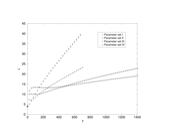
Figure 1: Evolution of the average domain size for parameter sets I, II, III, and IV (cf. Table 1) with the time step. Error bars are included and represent the uncertainty transmitted from the standard error of the structure function spherical average. Lattice size is $128^{3}$. All quantities are reported in lattice units.

Figure 2: Log-log plot of reduced length versus reduced time for the $128^{3}$-lattice data sets. Error bars are included. The four data sets correspond to parameter sets I, II, III, and IV (cf. Table 1), from left to right. Viewed from a grazing angle, one can see that a simple, algebraic interpolating curve is not truly obtainable here. The first few points of each set correspond to diffusive, zero-growth stages. The units on both axes are dimensionless.

5.2 Structure function

For parameter set I (cf. Table 1) we show in Fig. 3 a family of spherically-averaged structure functions versus wavenumbers, corresponding to time steps 200, 400, 600, 800, 1000, 1200, and 1400, from right to left. Just as in scattering cross-section measurements [17], we observe the peaks to grow and approach small wavenumbers as time evolves. In Figs. 4 and 5 we show the same family of curves using time steps as absissae and wavenumbers as parameters. Regions of linear growth with time on such a logarithmic scale indicate that a diffusive process is dominating the dynamics. In fact, an exponential time growth for the structure function shortly after the quench below the spinodal curve was predicted from the linearised Cahn-Hilliard Model-B equations without noise [17], which although incorporating order-parameter conservation, does not include hydrodynamics. This Cahn-Hilliard equation might be applicable to regimes in our fluid where hydrodynamic effects were unimportant, as in the initial stages. Assuming linear perturbations $\phi^{\prime}$ to the order parameter, Cahn predicted that for fluctuations of small amplitude and long wavelength there is an instability of the shape

$$S(k,t)=S(k,0)\mathrm{e}^{-2\omega(k)t}$$ (39)

for $k<k_{c}$, where $k_{c}$ depends on the diffusion constant. Here, $t$ is the time, $\omega(k)<0$, and $S(k,t)\propto\langle\Big{|}\phi_{\mathbf{k}}^{\prime}(t)\Big{|}^{2}\rangle$, the brackets denoting averaging in reciprocal space over a shell of radius $k$.

Exponential growth occurs in our simulations as can be seen from Figs. 4 and 5 for about the first 350 time steps for most of the wavenumbers, indicating its transient character. The plateau of Fig. 1, Set I, lasts during the first 400 time steps, and we can see, Fig. 3, that up to 400 time steps the peak in the structure factor varies in height and very little in wavenumber, and is located at 0.491 (lattice units). This leads us to think that at these early stages the dynamics is mainly making walls thinner while average domain sizes barely change. In addition, visual inspection of the order parameter confirms the latter and suggests that hydrodynamic currents are weak, leaving diffusion as the mechanism leading the phase segregation process. When we check the structure function temporal evolution, Figs. 4 and 5, for the curves at and around $k=0.491$, we see that up to exactly 400 time steps do they show exponential growth, as the Cahn-Hilliard Model B predicts for a diffusive scenario. Also, exponential growth does not hold for all wavenumbers, but only for those smaller than about 0.7, in agreement with the existence of an upper cutoff for the validity of Eq.(39), predicted from Model B.

However, not all the wavenumbers follow Model B’s predictions, namely, that exponential growth is a transient and occurs up to a threshold wavenumber. In fact, exponential growth holds for all the time steps of the simulation for the larger length scales (wavenumbers up to about 0.245), suggesting that diffusion never ceases to dominate their dynamics. Also, exponential growth is seen for very small domain sizes (wavenumbers larger than 0.736) for time steps well advanced in the coarsening dynamics, after 600 time steps. These wavenumbers are close to and above the expected Model-B upper cutoff for exponential growth, set by the change in slope from positive to negative in Fig. 5. These departures from Model B’s predictions hold nonetheless for domain sizes far from the first moment of the structure factor, which is close to its peak and is our average domain size measure. It would be desirable in future works to investigate diffusional processes at $k<0.245$ for all of the simulation time, and $k>0.736$ at late times: according to the Cahn-Hilliard linearised Model B, for these cases diffusion is negligible or forbidden, respectively.

Analogous behaviour to Fig. 3 is exhibited for parameter sets II, III, and IV (cf. Table 1) in Figs. 6, 7, and 9, respectively. For the last two time slices taken in Fig. 9, the peaks seem no longer to drift to the left, as a result of finite size effects (arrest of domain growth). Regarding regions of exponential growth with time, the three data sets confirm Eq. (39), with an upper bound for $k$.

Figure 8 shows the collapse (matching) of the structure functions corresponding to parameter set III (cf. Table 1), for a $128^{3}$ lattice size and time steps from 450 to 700, when they are scaled by Eq. (8), the abscissae being rescaled by a factor of $(2\pi)^{-1}$, and the ordinates by the peak’s maximum. Earlier times are represented in Fig. 8 by empty symbols, and later times by filled symbols. There is good collapse, and, therefore, scaling according to the scaling hypothesis, in the region from $q=0.4$ to about $q\approx 3$, where $q\equiv kL$ is dimensionless. The middle of the region $1<q<2$ follows a $q^{-9}$ behaviour, in accordance with Tomita’s prediction of an exponent $-6$ or more negative [69].

Close to $q\approx 3$ we observe the presence of a shoulder, as has been reported in experiments [67] and numerical simulations [54, 68]. Most strikingly, the shape of our large-$q$ tail is very reminiscent of that of Fig. 4 in [54] and that of Fig. 3 in [68]: (1) there is still a time dependence indicating that interfaces have not yet been fully resolved (we are probing the smallest scales where diffusion still exists and $\xi/L$ is not small enough); and (2) the tail decreases with an exponent which is in fact more negative than that of the Porod tail, Eq. (6), despite what these authors [54, 68] claim.

For $q<0.4$, data points do not seem to collapse onto the same curve of those for $q>0.4$. This is similar to, but with more data than, the results of Koga and Kawasaki [68]. Our results show an exponent growing with time: the slope of a line (not shown) joining the first two empty circles ($T=450$) is 1.61, while the slope of a line (not shown) joining the last two filled downward triangles ($T=700$) is 2.12. This resembles the temporal growth cited by Appert et al. [54] on the results of Alexander et al. [35]; nonetheless, we consider the amount of data in the latter insufficient to draw firm conclusions. Given that the points at $T=700$ are closer to the asymptotic regime, we take such a slope as our best approximation to the asymptotic regime.

In the small-$q$ region, Yeung [61] predicted a $q^{4}$ behaviour for the asymptotic limit ($L\to\infty$, or at late times). Additionally, at earlier stages, a term proportional to $L^{-2}q^{2}$ caused by thermal noise would also come into play. Now, Appert et al.’s estimate [54] applies well for our results: such a quadratic term is less dominant than the quartic one only for $q>0.4$, given that the largest value of $L(T)$ for which there are no finite size effects is also about 25. This happens to be the region where we find the $q^{2}\leftrightarrow q^{4}$ crossover.

Fig. 10 shows similar curves for parameter set IV (cf. Table 1), where only time steps 450 to 675 are displayed and we have also normalised the curve such that the peak is located at (1,1). We have again neglected early time steps because of poor collapse. A fit to the tail in $2<q<10$ gives $q^{-3.65}$, close to being a Porod’s law. It is when we probe the finest length scales, at $q\approx 10$ that it ceases to apply, due to lattice discretisation effects.

The behaviour at intermediate wavenumbers is between $q^{-8}$ and $q^{-7}$, again in agreement with Tomita’s theory [69], and close to $q^{-7}$ as computed using a dissipative particle dynamics method by Jury et al. [11] and a lattice-gas automaton by Love et al. [7].

For small momenta (large domains) we found a behaviour close to $q^{3}$, in agreement with the numerical results of Love et al. [7] and in disagreement with Yeung’s predictions [61].

The most notable difference between Figs. 8 and 10 is the behaviour above $q\approx 1.5$. Figure 10 shows a neat Porod tail, which bends down dramatically for $q>10$, whereas Fig. 8 shows either a poor Porod tail in the region $3<q<5$, or a minute one in the region $1.5<q<3$. A condition assumed in the derivation of Porod’s law [19] is that the sampling length $r$ satisfies $\xi\ll r\ll L$, which in wavenumbers means

$$1/L\ll k\ll 1/\xi\,.$$ (40)

By ‘eyeball’ inspection of the system’s order parameter we found that interface widths naturally shrink with an increasing number of time steps, going from about 5 or 6 lattice unit spacings at 200 time steps down to about 3 at 675 time steps, regardless of the data set, III or IV (cf. Table 1). Simulations for a $256^{3}$ lattice size revealed similar widths, and snapshots of the order parameter at 200 and 700 time steps are shown in Figs. 11 and 12. With these widths in mind, assuming domain sizes of a quarter of the lattice side length (the threshold imposed by our prescription for eliminating finite size effects), and a $128^{3}$ lattice, the condition (40) becomes

$$1\ll q\ll 10\,,$$ (41)

which contains our large-$q$ region. Despite this, we do not observe a Porod tail for data set III, or, as in data set IV, the tail obtained is only close to being a Porod tail. This is in agreement with the fact Eq. 40 is necessary but not sufficient for a Porod tail to hold.

Finally, it is worth noting in Fig. 12 the existence of nested domains and droplets much smaller than the average domain size.

x

Figure 3: Spherically averaged structure function versus wavenumber, for parameter set I (cf. Table 1). $128^{3}$ lattice. Error bars represent the standard error of the structure function spherical average. Time slices shown are time step 200, 400, 600, 800, 1000, 1200, and 1400 from right to left. All quantities are reported in lattice units.

Figure 4: Evolution of the spherically averaged structure function with the time step for parameter set I and a $128^{3}$ lattice, on a logarithmic scale. When observed along the ordinate $T=200$, the curves correspond to wavenumbers $k=0.147$, 0.196, 0.245, 0.295, 0.344, 0.393, and 0.442 from bottom to top, respectively. Error bars represent the standard error of the structure function spherical average. Regions of linear growth are those for which the exponential behaviour Eq.(39) holds. For wavenumbers up to 0.2 exponential and therefore diffusive behaviour is seen for all the simulation time. For larger wavenumbers (and hence smaller domain sizes) diffusion occurs as a transient. All quantities are reported in lattice units.

Figure 5: Similar to Fig 4, but the curves correspond to wavenumbers $k=0.491$, 0.540, 0.589, 0.638, 0.687, 0.736, 0.785, and 0.834 from top to bottom, respectively. We can see that linear growth ceases to hold for wavenumbers larger than about 0.736, in accordance with existence of an upper cutoff for the validity of Eq. (39). All quantities are reported in lattice units.

Figure 6: Spherically averaged structure function versus wavenumber, for parameter set II (cf. Table 1). $128^{3}$ lattice. Error bars represent the standard error of the structure function spherical average. Time slices shown are time step 200, 400, 600, 800, 1000, 1200, and 1400 from right to left. All quantities are reported in lattice units.

Figure 7: Spherically averaged structure function for parameter set III (cf. Table 1). $128^{3}$ lattice. Error bars represent the standard error of the structure function spherical average. Time slices shown are time step 100, 200, 300, 400, 500, 600, and 700 from right to left. All quantities are reported in lattice units.

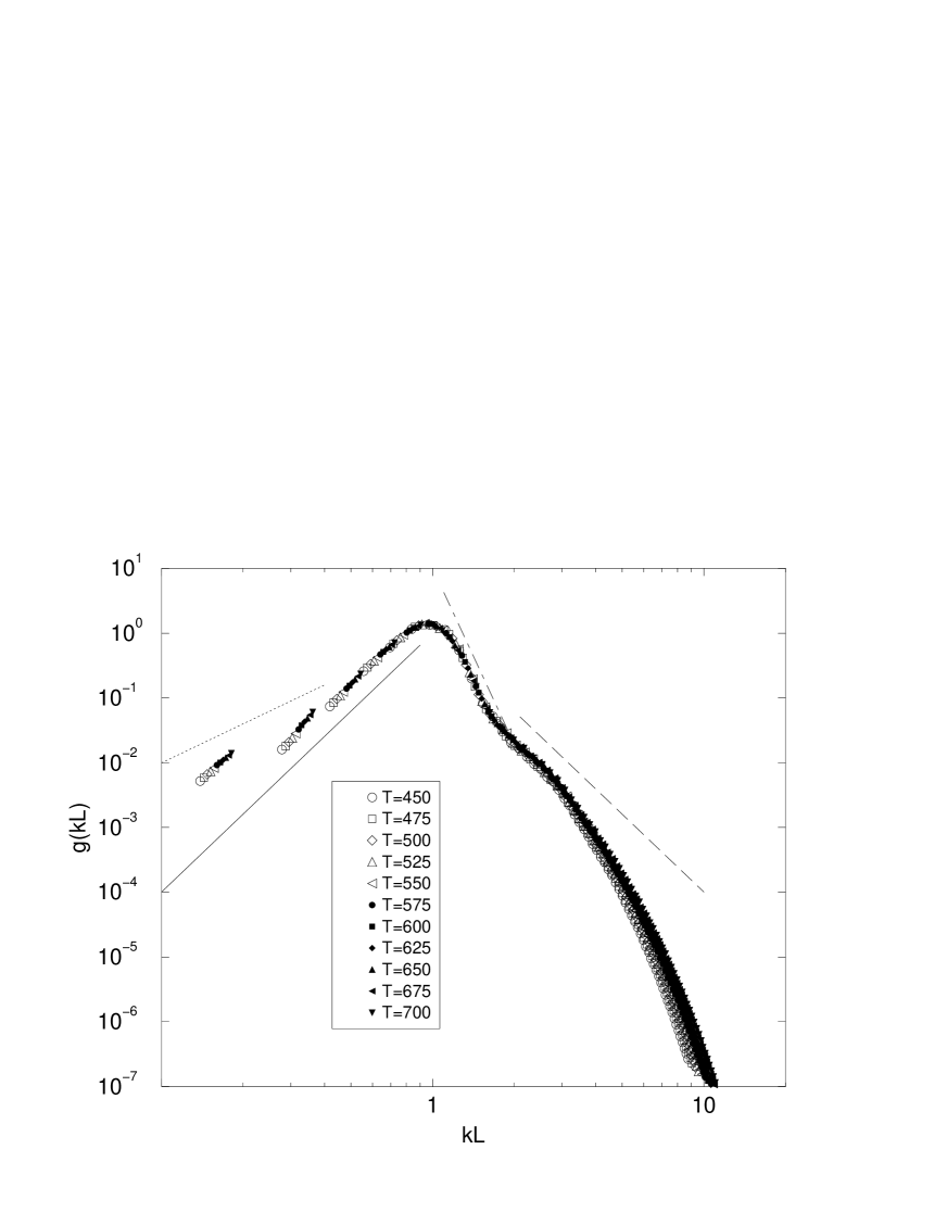
Figure 8: Scaled spherically averaged structure function for parameter set III (cf. Table 1), as defined by Eq. (8). Lattice size is $128^{3}$. Time steps are as shown in the legend. Earlier times correspond to the empty symbols; later times to the filled symbols. Error bars are smaller than the size of the symbols. Straight lines serve as slope guides to the reader only, and represent power laws $q^{2}$, $q^{4}$, $q^{-9}$, and Porod’s law $q^{-4}$, from left to right, respectively, with $q\equiv kL$. All quantities are reported in lattice units.

Figure 9: Spherically averaged structure function versus wavenumber, for parameter set IV (cf. Table 1). $128^{3}$ lattice. Error bars represent the standard error of the structure function spherical average. Time steps shown are 100, 200, 300, 400, 500, 600, and 675, from right to left. All quantities are reported in lattice units.

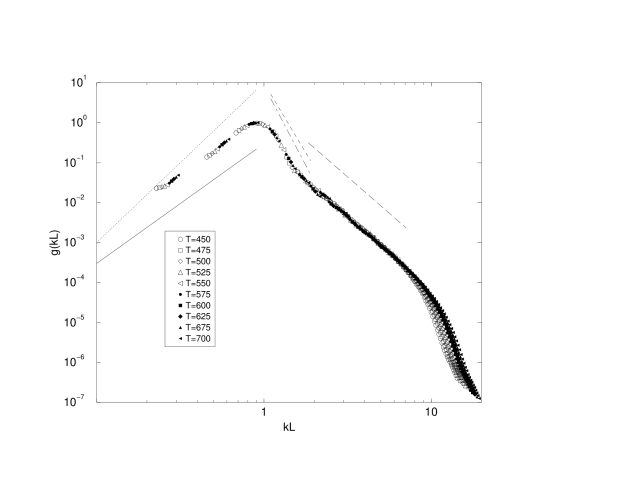
Figure 10: Scaled spherically averaged structure function for parameter set IV (cf. Table 1), as defined by Eq. (8). Lattice size is $128^{3}$. Time steps shown are from 450 up to 675, every 25. Earlier times correspond to the innermost lines; later times to the outermost lines. Error bars are smaller than the size of the symbols, except for the two leftmost, detached data sets, for which they are slightly larger. Straight lines serve as slope guides to the reader only, and represent power laws $q^{3}$, $q^{4}$, $q^{-8}$, $q^{-7}$, and the fit to the large-$q$ tail, $q^{-3.65}$, from left to right, respectively, with $q\equiv kL$. All quantities are reported in lattice units.

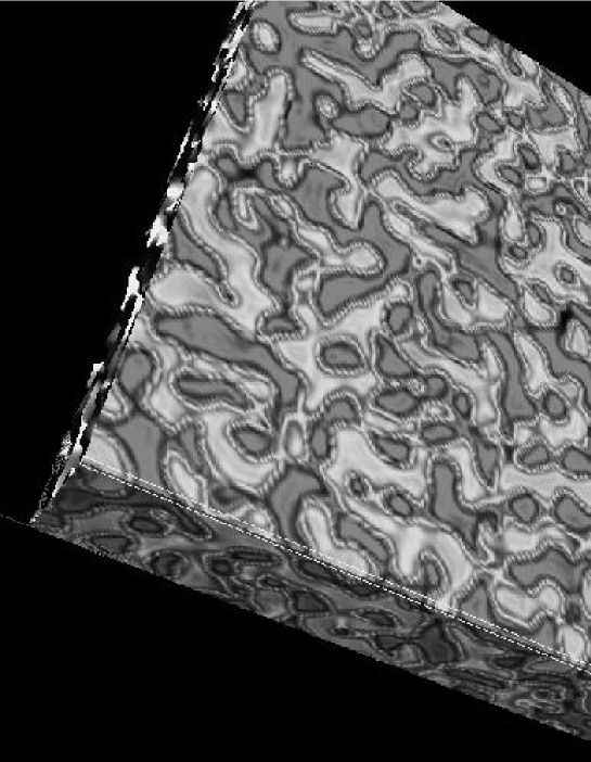
Figure 11: Order parameter ($\rho^{R}-\rho^{B}$) snapshot at time step 200 for parameter set IV (cf. Table 1). We show a slab of the $256^{3}$ lattice simulated.

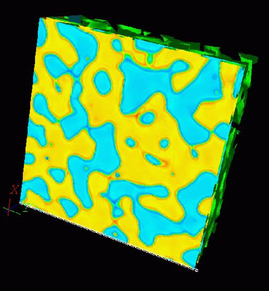
Figure 12: Order parameter ($\rho^{R}-\rho^{B}$) snapshot at time step 700 for parameter set IV (cf. Table 1). We show a slab of the $256^{3}$ lattice simulated.

6 Numerical stability of our lattice-Boltzmann algorithm

As is well known, owing to the lack of an H-theorem, an approach to equilibrium is not guaranteed in all lattice-Boltzmann models to date; recent theoretical developments to address and solve this have been made [42, 43, 44]. For single-phase lattice-Boltzmann models, equilibrium states are well defined in the collision term; if the automaton does relax to these, the pertinent macroscopic momentum (and sometimes energy) balance equations are reproduced in the low-Knudsen number limit. Interacting, multicomponent lattice-Boltzmann models exhibit the same situation in the bulk of pure fluid regions where intercomponent interactions are negligible. For regions where they are not, there is not even a well-established thermohydrodynamic theory which could provide equilibria to which the automaton could relax to, or with which to compare the stationary state to which it can evolve. Whether dealing with a single or multiphase system, lattice-BGK stationary regimes ought to be treated with caution and contrasted with experiment.

Numerical instabilities are the reflection of the lack of an H-theorem, which is a direct consequence of space and time discretisation on the BGK-Boltzmann equation and the freedom in the choice of the equilibrium distribution function [44]. These instabilities can be defined as follows. As is generally the case for a finite difference method with a single relaxation parameter, such as our lattice-BGK model for a zero phase-coupling constant [41], linear stability occurs within a finite interval of such a parameter. If multicomponent interactions are introduced, additional parameters may influence the stability: density, intercomponent coupling strength, and even composition. The mechanism is simple: certain choices of parameters can turn the lattice-BGK collision term positive (therefore increasing the mass density) for long enough to generate floating-point numbers larger than the largest the machine can deal with, hence causing an overflow signal. Numerical instabilities are defined in this work as the generation of such floating-point numbers. We consider it crucial to be able to map out regions in the model’s parameter space leading to unstable configurations, and to report them alongside any lattice-BGK simulations.

Using the same initial conditions as explained in Section 5, we found our algorithm to be unstable for regimes with the smallest length and time scales, $L_{0}$ and $T_{0}$, which coincide with those of the largest Mach numbers. In Table 3 we show some of the paramaters leading to numerical instability. The dependence of the surface tension on the model parameters, as given in Section 4, should be taken into consideration as a guide to steering through the parameter space. Note that all values of $\Delta t$ included are larger than that for parameter set IV.

$\rho$	$\tau$	$g$	$\sigma(\rho,\tau,g)$	$T_{0}$
0.5	0.5625	0.06	0.0115	0.0169
0.5	0.5625	0.03	0.0052	0.0122
0.3	0.5625	0.10	0.0068	0.0174
0.3	0.5500	0.08	0.0061	0.0112

Table 3: Model parameters leading to numerical instability, including the surface tension $\sigma(\rho,\tau,g)$ generated some time steps before the instability sets in, and the associated characteristic time. The lattice used was $4\times 4\times 128$, and the instability sets in before 4000ts.

We then investigated the nature of our instabilities, as others have done. The group of Cates found troublesome numerical instabilities with their free-energy based, lattice-BGK model in 3D in regions in which quiescent binary portions of fluid go into a checkerboard state [27]. They reported that their model is unconditionally unstable [26]. Nonetheless, by improving the way gradients were treated numerically they were able to considerably reduce this unphysical behaviour. For our model, we looked at the time evolution of the quantity

$$\theta(t)\equiv\max\{|\Omega_{k}^{\prime\alpha}({\mathbf{x}},t)|\,,\,\,\forall{\mathbf{x}},\forall k,\forall\alpha\}\,,$$ (42)

for parameters $\{\rho=0.3,\,g=0.06,\,\tau=0.5125\}$, where the collision term, $\Omega_{k}^{\prime\alpha}$, is defined in Eq. (25). We also monitored the maximum and average values of the fluid mixture’s speed, $u_{\mathrm{max}}$ and $\overline{u}$, respectively, on the lattice. We show these quantities for a $32^{3}$ lattice in Figs. 13, 14 and 15. We see how $\theta$ reverses its decreasing trend in a few time steps; after that, it blows up at $T=52$ time steps. We only show data up to $T=49$, as $\theta(T=51)\approx 10^{111}$. $u_{\mathrm{max}}$ blows up in similar style: at $T=50$, $u_{\mathrm{max}}=7498$ and $\theta\approx 10^{21}$; at $T=51$, $u_{\mathrm{max}}$ has exceeded the maximum floating-point value that the computer can deal with, and overflow signals are generated. This indicates that at the time steps immediately prior to the onset of the instability the lattice gets more and more populated with increasing speeds until in two or three time steps they grow by ten or more orders of magnitude. That the population of lattice sites with rapidly increasing speeds over time is small compared to the lattice volume can be concluded from contrasting the time variation in the standard error (“one sigma”) of ${\overline{u}}$ to the time variation of ${\overline{u}}$, Fig. 15. The same parameter set run on a $128^{3}$ lattice seems to make the instability set in much quicker, as it occurs during the first 10 time steps. As a final check, we ran a $128^{3}$ lattice with parameter set I (cf. Table 1) for 20000 time steps and found no instabilities. The time evolution of $\theta$, $u$ and $\overline{u}$ is shown in Figs. 16, 17 and 18, respectively. We conclude that the occurrence of instabilities only depends on the set of parameters used, regardless of the number of time steps simulated.

Figure 13: Evolution of the collision term maximum absolute value, $\theta$, Eq.(42), with the time step on a $32^{3}$ lattice for parameters $\{\rho=0.3,\,g=0.06,\,\tau=0.5125\}$. The interpolating curve serves as a guide to the eye only. All quantities are in lattice units.

Figure 14: Evolution of the maximum speed, $u_{\mathrm{max}}$, with the time step on a $32^{3}$ lattice for parameters $\{\rho=0.3,\,g=0.06,\,\tau=0.5125\}$. The interpolating curve serves as a guide to the eye only. All quantities are in lattice units.

Figure 15: Evolution of the speed average, $\overline{u}$, with the time step on a $32^{3}$ lattice for parameters $\{\rho=0.3,\,g=0.06,\,\tau=0.5125\}$. Error bars represent the standard error of the average (“one sigma”). All quantities are in lattice units.

Figure 16: Evolution of the collision term maximum absolute value, $\theta$, Eq.(42), with the time step on a $128^{3}$ lattice for parameter set I (cf. Table 1). We can see a decreasing trend for most of the simulation, which accentuates after time step 10000. The interpolating curve serves as a guide to the eye only. All quantities are in lattice units.

Figure 17: Behaviour of the maximum speed, $u_{\mathrm{max}}$, with the time step for a $128^{3}$ lattice with parameter set I (cf. Table 1). It shows an overall decreasing trend. The interpolating curve serves as a guide to the eye only. All quantities are in lattice units.

Figure 18: Evolution of the speed average, $\overline{u}$, with the time step on a $128^{3}$ lattice for parameter set I (cf. Table 1). We can see a decreasing trend of the average and its error. All quantities are in lattice units.

7 Conclusions

We have presented a quantitative study of the phase separation dynamics in three dimensions for critical (50:50) fluid mixtures (spinodal decomposition) for a modified Shan-Chen lattice-BGK model of multicomponent, isothermal immiscible fluids.

We found that after a brief diffusional transient in which interconnected regions of fluid species embedded into one another are formed, the average size of such regions grows with time as $l\propto t^{\gamma}$, where $\gamma\approx 2/3$. The trend is for the value to increase in the range $0.545\pm 0.014<\gamma<0.717\pm 0.002$ as the Reynolds number increases. This increase is consistent with a crossover from $l\propto t^{1/3}$ diffusive behaviour to hydrodynamic viscous growth $l\propto t$ predicted by the Cahn-Hilliard Model H. Owing to the significant amount of diffusion present at low Reynolds number, we do not consider our results to be indicative of a genuinely hydrodynamic inertial $t^{2/3}$ regime.

We observed exponential growth in the time dependence of the structure function for wavenumbers up to a threshold value, in qualitative agreement with predictions from the linearised Cahn-Hilliard Model B. For small wavenumbers, such an exponential growth is seen at all simulation times, whereas it is only an initial transient for larger wavenumbers. These departures from Model B predictions are for wavenumbers far from the one characterising the average domain size. A natural continuation of this work would be to investigate the nature of diffusion currents for these cases.

We have found very good agreement with the dynamical scaling hypothesis in the form of a neat collapse of the structure function curves for $\mathrm{Re}=2.7$ and $\mathrm{Re}=37$ when they are appropriately scaled according to Eq. (8). This collapse holds roughly for the second half of the simulation time, as diffusional transients act during the first. By looking at order parameter snapshots we observed the formation of nested domains and smaller droplets for the largest Reynolds numbers achieved, as Wagner and Yeomans also found [10]. However, unlike them, in our case these are transients rather than a result of length scales growing at different speeds, as poor collapse of the scaling functions would then occur due to breakdown of scale invariance.

Yeung predicted a $q^{2}$ behaviour at the small-$q$ end of the spectrum as the result of thermal effects at pre-asymptotic stages [61]. Love et al. [7] conjectured that a $q^{2}$ behaviour, and a crossover to $q^{4}$, could be caused by (a) lattice-gas noise, or (b) a poor scaling collapse, and that their $t^{2/3}$ domain growth, instead of $t$, might be justified by the former. Appert et al. [54] ascribed the $q^{2}$ behaviour and the crossover to not having reached the asymptotic limit, $L\to\infty$ (poor scaling collapse again). Our noiseless model reproduced the $q^{2}\leftrightarrow q^{4}$ crossover at $\mathrm{Re}=2.7$ and did not at $\mathrm{Re}=37$, for which there is better scaling collapse, and also produced a 2/3 domain growth (crossover) exponent. All this leads us to conclude that noise may not play as important a role as the lack of scaling collapse in explaining the $q^{2}\leftrightarrow q^{4}$ crossover, and is definitely not a requirement for the reproduction of a 2/3 domain growth exponent. A $q^{2}$ behaviour is the only one experimentally observed by Kubota et al. [67] for a mixture of isobutyric acid and water; they cite surface tension effects, measurement difficulties, multiple light scattering, and even specificity to the mixture’s molecular weight as reasons for not seeing a $q^{4}$ behaviour, and definitely discard thermal noise. Not surprisingly, in his prediction Yeung assumed a diffusive domain growth exponent of $1/3$, which is rather seen in quenches of polymer mixtures and metal alloys.

In the case $\mathrm{Re}=37$, the spectrum shows a $q^{3}$ behaviour in the small-$q$ limit, in disagreement with Yeung’s prediction. In fact, his analysis is based on a Cahn-Hilliard model without hydrodynamics.

The numerical instabilities seen in our runs are caused by large speeds turning the equilibrium distribution negative for long enough to incur floating-point overflows. This happens for characteristic times (cf. Table 1) below $T_{0}=0.0172$, and the population of lattice sites undergoing such a burst in the fluid’s macroscopic speed is small compared to the lattice volume. We found no evidence that an initially stable regime becomes unstable at later times, as typically happens in relaxational models (such as is our model for $g_{\alpha\overline{\alpha}}=0$). This is in stark contrast with the findings of Kendon et al. [26] and Cates et al. [27] in their spinodal decomposition studies using a free-energy based, lattice-BGK model, who reported their algorithm to be unconditionally unstable.

A search for a crossover to growth laws other than $t^{2/3}$ at Reynolds numbers higher than $\mathrm{Re}=37$ faces two major problems: (a) the triggering of numerical instabilities due to large inter-species coupling and smallness of relaxation time values; and (b) the approach to the compressible limit, whose macrodynamic behaviour for pure phases cannot, by construction, be correctly described by our method. On the other hand, there is still scope to achieve Reynolds numbers smaller than $\mathrm{Re}=0.18$ in search of the end of the crossover to $t^{1/3}$. Closeness to the miscibility threshold may make this endeavour difficult, as it is reached for characteristic times ca. $T_{0}=1.43\times 10^{8}$.

Our results clearly challenge the claim that a domain growth linear with time is universal for all models of phase separating fluids sharing similar values of $L_{0}$ and $T_{0}$ since we obtained excellent collapse of scaled structure functions yet our domain growth exponents are in the crossover region between diffusive and hydrodynamic viscous regimes.

The properties of this binary immiscible fluid model are important for underpinning the more complex domain growth observable in ternary amphiphilic (oil/water/surfactant) fluids we expect to report in forthcoming publications.

8 Acknowledgments

This work was supported by EPSRC grants GR/M56234 and RealityGrid GR/R67699 which provided access to Cray T3E-1200E, SGI Origin2000 and SGI Origin3800 supercomputers at Computer Services for Academic Research (CSAR), Manchester University, UK, and by the Center for Computational Science, Boston University, USA, through a collaborative project to access their several SGI Origin2000 platforms. We also thank the Higher Education Funding Council for England (HEFCE) for our on-site 16-node SGI Onyx2 graphical supercomputer. We wish to thank Dr Hudong Chen and Dr Peter J Love for useful discussions, Mr Jonathan Chin for implementing the parallel code, and Dr Keir Novik for technical assistance. NGS also wishes to thank Dr Ignacio Pagonabarraga for useful discussions, and Prof David Jou, Prof José Casas-Vázquez and Dr Juan Camacho at the Universitat Autònoma de Barcelona, Spain, for their support.

References

- [1] F. Perrot, P. Guenoun, T. Baumberger, D. Beysens, Phys. Rev. Lett. 73, 688 (1994).
- [2] F. Perrot, D. Beysens, Y. Garrabos, T. Frölich, P. Guenoun, M. Bonetti, and P. Bravais, Phys. Rev. E 59, 3079 (1999).
- [3] M. Grant, M. San Miguel, J. Viñals, and J. D. Gunton, Phys. Rev. B 31, 3027 (1985).
- [4] F. J. Solis and M. Olvera de la Cruz, Phys. Rev. Lett. 84, 3350 (2000).
- [5] A. Chakrabarti, R. Toral, and J. D. Gunton, Phys. Rev. B 39, 4386 (1989).
- [6] O. T. Valls and J. E. Farrell, Phys. Rev. E 47, R36 (1993).
- [7] P. J. Love, P. V. Coveney, and B. M. Boghosian, Phys. Rev. E 64, 021503 (2001).
- [8] A. N. Emerton, P. V. Coveney, and B. M. Boghosian, Phys. Rev. E 55, 708 (1997).
- [9] V. M. Kendon, J.-C. Desplat, P. Bladon, and M. E. Cates, Phys. Rev. Lett. 83, 576 (1999).
- [10] A. J. Wagner and J. M. Yeomans, Phys. Rev. Lett. 80, 1429 (1998).
- [11] S. Jury, P. Bladon, S. Krishna, and M. E. Cates, Phys. Rev. E 59 R2535 (1999).
- [12] M. Laradji, S. Toxvaerd, and O. G. Mouritsen, Physica A 239, 404 (1997).
- [13] For a recent review see S. Chen and G. D. Doolen, Annu. Rev. Fluid Mech. 30, 329 (1998).
- [14] X. Shan and H. Chen H, Phys. Rev. E 47, 1815 (1993); X. Shan and H. Chen, Phys. Rev. E 49, 2941 (1994).
- [15] M. R. Swift, W. R. Osborn, and J. M. Yeomans, Phys. Rev. Lett. 75, 830 (1995); M. R.Swift, E. Orlandini, W. Osborn, and J. M. Yeomans, Phys. Rev. E 54 5041 (1996).
- [16] A. J. Wagner and J. M. Yeomans, Phys. Rev. E 59, 4366 (1999).
- [17] J. D. Gunton, M. San Miguel, and P. S. Sahni, in Phase Transitions and Critical Phenomena, Vol. 8, edited by C. Domb and J. Lebowitz (Academic Press, New York, 1983).
- [18] A. Balazs, Current Opinion in Colloid & Interface Science 4, 443 (2000).
- [19] A. J. Bray, Adv. Phys. 43, 357 (1994).
- [20] J. H. Ferziger and H. G. Kaper, in Mathematical theory of transport processes in gases (North Holland, Amsterdam, 1972).
- [21] N. González-Segredo, M.Phil. thesis, Universitat Autònoma de Barcelona, 1997; H. Grad, Comm. Pure Appl. Math. 2, 331 (1949).
- [22] M. Nekovee, P. V. Coveney, H. Chen, and B. M. Boghosian, Phys. Rev. E 62, 8282 (2000).
- [23] X. He and L.-S. Luo, Phys. Rev. E 56, 6811 (1997).
- [24] U. Frisch, D. d’Humières, B. Hasslacher, P. Lallemand, Y. Pomeau, and J.-P. Rivet, Complex Systems 1, 649 (1987).
- [25] M. E. Cates, V. M. Kendon, P. Bladon, and J.-C. Desplat, Faraday Disc. Roy. Chem. Soc. 112, 1 (1999) (Also: arXiv:cond-mat/9908007).
- [26] V. M. Kendon, M. E. Cates, I. Pagonabarraga, J.-C. Desplat, and P. Bladon, J. Fluid Mech. 440, 147 (2001).
- [27] M. E. Cates. Private communication (2001).
- [28] I. Pagonabarraga, J.-C. Desplat, A. J. Wagner, and M. E. Cates, New Journal of Physics 3, 9.1 (2001) (http://www.njp.org/).
- [29] H. Tanaka, Phys. Rev. Lett. 72, 3690 (1994).
- [30] J. Chin and P. V. Coveney, Phys. Rev. E 66 016303 (2002).
- [31] T. Araki and H. Tanaka, Macromolecules 34 1953 (2001).
- [32] In practice, some systems require a level of description that the lattice-Boltzmann mesoscopic dynamics cannot lend, and averaging over independent initial conditions is carried out. See, for example, G. D. Doolen, T. Clark, and E. Ben-Naim, in Universal fluctuation statistics for the Rayleigh-Taylor interface, Europhysics Conference Abstracts (Volume 25H) of the International Conference on Discrete Simulation of Fluid Dynamics, Institut d’Etudes Scientifiques de Cargèse, Corsica, July 2001, edited by J. P. Boon, P. V. Coveney, and S. Succi (European Physical Society).
- [33] An in-depth explanation of Model B and Model H, among others is: P. C. Hohenberg, Rev. Mod. Phys. 49, 435 (1977).
- [34] N. S. Martys and J. F. Douglas, Phys. Rev. E 63, 031205 (2001).
- [35] F. J. Alexander, S. Chen, and D. W. Grunau, Phys. Rev. B 48, 634 (1993).
- [36] A. K. Gunstensen, D. H. Rothman, S. Zaleski, and G. Zanetti, Phys. Rev. A 43, 4320 (1991).
- [37] J. S. Rowlinson and B. Widom, in Molecular theory of capillarity (Clarendon Press, Oxford, 1982).
- [38] T. Inamuro, N. Konishi, and F. Ogino, Comp. Phys. Comm. 129, 32 (2000).
- [39] J. D. Sterling and S. Chen, J. Comp. Phys. 123 196 (1996).
- [40] P. Lallemand and L.-S. Luo, Phys. Rev. E 61, 6546 (2000).
- [41] Y. H. Qian, D. d’Humières, and P. Lallemand, Europhys. Lett. 17, 479 (1992).
- [42] I. V. Karlin, A. Ferrante, and H. C. Öttinger, Europhys. Lett. 47, 182 (1999).
- [43] H. Chen and C. Teixeira, Comp. Phys. Comm. 129, 21 (2000).
- [44] B. M. Boghosian, J. Yepez, P. V. Coveney, and A. Wagner, Proc. Roy. Soc. Lond. A 457, 717 (2001).
- [45] B. M. Boghosian, Peter J. Love, Peter V. Coveney, Iliya V. Karlin, Sauro Succi, and Jeffrey Yepez, http://arXiv.org/abs/cond-mat/0211093.
- [46] U. Frisch, D. d’Humières, B. Hasslacher, P. Lallemand, Y. Pomeau, and J.-P. Rivet, Complex Systems 1, 649 (1987); D. H. Rothman and J. M. Keller, J. Stat. Phys. 52, 1119 (1988); G. D. Doolen (ed.), Physica D 47 (1991); C. Appert and S. Zaleski, Phys. Rev. Lett. 64, 1 (1990).
- [47] P. J. Hoogerbrugge and J. M. V. A. Koelman, Europhys. Lett. 19, 155 (1992); E. G. Flekkøy and P. V. Coveney, Phys. Rev. Lett. 83, 1775 (1999).
- [48] K. E. Novik and P. V. Coveney, Phys. Rev. E 61, 435 (2000).
- [49] P. Fratzl, O. Penrose, R. Weinkamer, and I. Žižak, Physica A 279, 100 (2000).
- [50] G. K. Batchelor, An introduction to fluid dynamics (Cambridge University Press, Cambridge, UK, 1967).
- [51] W. Cahn and J. E. Hilliard, J. Chem. Phys. 28, 258 (1958).
- [52] H. E. Cook, Acta Metall. 18, 297 (1970).
- [53] G. Tryggvason, B. Bunner, O. Ebrat, W. Tauber, in Computations of Multiphase Flows by a Finite Difference/Front Tracking Method. I Multi-Fluid Flows, 29th Computational Fluid Dynamics Lecture Series 1998-03 (Von Karman Institute for Fluid Dynamics) (Available from http://www-personal.engin.umich.edu/~gretar.)
- [54] C. Appert, J. F. Olson, D. H. Rothman, and S. Zaleski, J. Stat. Phys. 81, 181 (1995).
- [55] J. E. Farrell and O. T. Valls, Phys Rev B 40, 7027 (1989).
- [56] I. Pagonabarraga, A. Wagner, and M. E. Cates, Preprint (2001). (arXiv:cond-mat/0103269.)
- [57] I. Pagonabarraga. Private communication (2001).
- [58] M. Nekovee, J. Chin, N. González-Segredo, and P. V. Coveney, in Computational Fluid Dynamics, Proc. 4th UNAM Supercomputing Conference, Mexico D. F., 27-30 June 2000, edited by E. Ramos, G. Cisneros, R. Fernández-Flores, and A. Santillán-González (World Scientific, Singapore, 2001.)
- [59] L.-S. Luo, Phys. Rev. Lett. 81, 1618 (1998).
- [60] N. Martys, X. Shan, and H. Chen, Phys. Rev. E 58, 6855 (1998).
- [61] C. Yeung, Phys. Rev. Lett. 61, 1135 (1998).
- [62] H. Furukawa, Adv. Phys. 34, 703 (1993).
- [63] W. H. Press, S. A. Teukolsky, W. T. Vetterling, and B. P. Flannery, in Numerical Recipes in C. The Art of Scientific Computing, 2nd edition, software version 2.08 (Cambridge University Press, Cambridge, UK, 1999.)
- [64] http://www.faqs.org/rfcs/rfc1014.html; Unix manual pages (% man xdr).
- [65] http://www.avs.com.
- [66] The limit , , , with both mean free path and fixed, where stands for the number of particles, is their mass, and is the range of the interparticle, hard-sphere potentials, was baptised ‘the Boltzmann-Grad limit’ by O. E. Landford III. In addition, the density has to be sufficiently low so that only binary collisions need be considered (consequence of ), and spatial gradients small enough such that collisions can be thought of as localised in space. The most rigorous proof that in this limit the Stosszahlansatz, and therefore the Boltzmann equation (without a body force term), is exact for at least short times was provided by Landford in 1981 (Physica A 106, 70 (1981)), the system described being an ideal gas. In 1985 Reinhard Illner and Mario Pulvirenti extended the result to three dimensions (c.f. C. Cercignani, R. Illner and M. Pulvirenti, in The mathematical theory of dilute gases, Applied Mathematical Sciences 106 (Springer-Verlag, New York, 1994)). See also http://www.ann.jussieu.fr/publications/1995/R95026_Perthame.ps.gz for a list of references on collision models in Boltzmann’s theory.
- [67] K. Kubota, N. Kuwahara, H. Eda, and M. Sakazume, Phys. Rev. A 45, R3377 (1992).
- [68] T. Koga and K. Kawasaki, Phys. Rev. A 44, R817 (1991).
- [69] H. Tomita, Prog. Theor. Phys. 75, 482 (1986).