Gaussian factor in the distribution arising from the nonextensive statistics approach to fully developed turbulence

Abstract

We propose a simple modification, the Gaussian truncation, of the probability density function which was obtained by Beck (2001) to fit the experimental distribution of fluid particle acceleration component from fully developed fluid turbulence inspired by the framework of nonextensive statistical mechanics with the underlying gamma distribution of the model parameter. The modified distribution is given a phenomenological treatment and provides a good fit to new experimental results on the acceleration of fluid particle reported by Crawford, Mordant, and Bodenschatz. We compare the results with the new fit which was recently obtained by Beck (2002) with the use of the underlying log-normal distribution of the model parameter.

1 Introduction

Recently, C. Beck [1] have studied application of Tsallis nonextensive statistics formalism [2] to turbulent flows and achieved a good agreement with the high-precision Lagrangian data on the component of acceleration measured by Porta, Voth, Crawford, Alexander, and Bodenschatz [3]. Remarkably, no fit parameters have been used by Beck to reproduce distribution of the acceleration $a$ of a tracer particle advected by the turbulent flow, while the stretch exponential fit provides an excellent agreement with the experiment but requires three free parameters for this purpose [3, 4],

$$P(a)=C\exp\left[-a^{2}/[(1+\left|{b_{1}a}/{b_{2}}\right|^{b_{3}})b_{2}^{2}]\right],$$ (1)

where $b_{1}=0.513\pm 0.003$, $b_{2}=0.563\pm 0.02$, and $b_{3}=1.600\pm 0.003$ are fit parameters, and $C\simeq 0.733$ is a normalization constant. The big $|a|$ asymptotics is given by $P(a)\sim\exp[-|a|^{0.4}]$.

The main idea underlying the generalized statistical mechanics approach to the turbulence is simply to introduce fluctuations of the energy dissipation rate [5, 6] which follow gamma (chi-square) or some other appropriate distribution, into the stochastic dynamical model framework.

This type of models belongs to the class of purely temporal stochastic models of Lagrangian turbulence and corresponds to the universality of the developed turbulence which is expected to occur in the inertial range only statistically. Accordingly, velocity and acceleration of an individual fluid particle are treated as random variables, and one is interested in their time evolution and probability distribution functions, or multipoint correlation functions. By the universality (Kolmogorov 1941, Heisenberg 1948, Yaglom 1949), steady-state statistics of velocity increments in the inertial range and statistics of acceleration do not depend on details of the forcing and the dissipation (the dependence is postulated only via mean energy injection rate).

In a physical context, we describe fluid particle dynamics in statistically homogeneous and isotropic turbulence in terms of a Brownian like motion. Such models are formulated in the Lagrangian frame and naturally employ Langevin type equation and the associated Fokker-Planck equation, which can be derived under certain assumptions either in Stratonovich or Ito formulations. Under the stationarity condition, a balance between the energy injected at the integral scale and the energy dissipated by viscous processes at the Kolmogorov scale, one can try to solve the Fokker-Planck equation to find stationary one-point probability density function of the variable. This function as well as its moments can then be compared with the Lagrangian experimental data and direct numerical simulations (DNS) of the three-dimensional Navier-Stokes equation.

In contrast to the usual Wiener process, the components of acceleration do not merely wander in a random way with a complete self-similarity at all scales but were found to reveal a highly intermittent behavior, which can be seen from a strongly non-Gaussian character of the experimental probability density function of acceleration component of the tracer particle [3, 4]. This requires a consideration of some specific Langevin type equation and assigning some specific properties to additive and multiplicative noises, which are used to model the force.

With the simple choice of white-in-time noises such models fall into the class of Markovian models allowing well established Fokker-Planck approximation while the consideration of finite-time correlated noises and memory effects requires a deeper analysis. Approximation of a short-time correlated noise by the zero-time correlated one is usually made due to the time scale hierarchy emerging due to physical analysis of the system and experimental data.

In the Lagrangian framework some known examples of such models are due to Sawford [7], Beck [1, 5, 8], and Reynolds [9]. In the Eulerian framework (fixed probe) Langevin type equations for the velocity increments in space and for logarithm of the stochastic energy dissipation rate have been recently considered by Renner et al. [10].

Specifically, the class of models considered in the present paper is featured by the introduction of random intensity of the additive noise and/or random drift coefficient (random intensity of a multiplicative noise, in a more general consideration) that was found to imply strongly non-Gaussian marginal distributions of the acceleration which are associated to the Lagrangian intermittency, a phenomenon that developed turbulent flows exhibit when considering Lagrangian velocity increments at small timescales. Effectively, this approach allows one to account for longtime effects which are known to be important in describing the Lagrangian intermittency [11]. The model parameter $\beta>0$ appears here as the ratio between the drift coefficient and intensity of the additive noise. The marginal distribution $P(a)$ is obtained by integrating out $\beta$ in the Gaussian distribution of the acceleration, $P(a|\beta)$, a stationary solution of the Fokker-Planck equation, under the assumption that $\beta$ follows some judiciously chosen distribution.

In general, this approach assumes two characteristic timescales, one associated to a short-time scale, of the order of Kolmogorov time $\tau_{\eta}$, and the other associated to a longtime scale, of the order of Lagrangian integral time $T_{L}$, in a way similar to that assumed in the Sawford model [7]. (The Sawford model yields however independent Gaussian distributions for Lagrangian accelerations and velocities with zero means and constant variances.) The Fokker-Planck equation makes a link between the stochastic dynamical treatment and statistical approach. We refer the reader to references [1, 5, 8] for details of this approach.

Earlier work on such type of models is due to Castaing, Gagne, and Hopfinger [12], referred to as the Castaing model, in which log-normal distribution of the variance of a Gaussian distributed intermittent variable has been used to derive the marginal distribution without reference to a stochastic dynamical equation.

It should be stressed that the class of one-dimensional Langevin toy models considered in the present paper suffers from the lack of physical interpretation of coefficients and additive noise in the context of the three-dimensional Navier-Stokes equation and turbulence; see, e.g., reference [18]. It is however quite a theoretical challenge to make a link between the Navier-Stokes equation and such surrogate Langevin models, which are, of course, far from being full statistical model of turbulent dynamics of fluid particle. Strong and nonlocal character of Lagrangian particle coupling due to pressure effects makes the main obstacle to derive turbulence statistics from the Navier-Stokes equation. Recent attempt in this direction is due to the Batchelor-Proudman type stochastic distortion theory approach to the Navier-Stokes equation by Laval, Dubrulle, and Nazarenko [13] from which one can draw parallels with the considered class of models.

In the present paper we suggest a simple modification of the chi-square model, a Gaussian truncation of the resulting power law distribution. We compare results of this model with those of the chi-square model and recently suggested log-normal model [8], and the experimental data on Lagrangian acceleration statistics. Our consideration is restricted to a stationary one-point distribution function. Two-point statistical analysis is of much interested and can be made elsewhere.

Despite the considered models are not provided by a direct link to the three-dimensional Navier-Stokes turbulence, they can be viewed as prototypical stochastic models to interpret statistical data on the recently measured tracer particle Lagrangian acceleration data. Here we note only that due to the Navier-Stokes equation in the Lagrangian frame the acceleration in the inertial range of fully developed turbulence is driven by the pressure gradient term which dominates the viscous term. This is confirmed by both the agreement between the acceleration measurements and DNS results on the pressure gradient, and recent verification of the longstanding Heisenberg-Yaglom scaling of a component of acceleration, $\langle a^{2}\rangle=a_{0}{\bar{u}}^{9/2}\nu^{-1/2}L^{-3/2}$, where ${\bar{u}}$ denotes root mean square (rms) velocity, for the Taylor microscale Reynolds numbers $R_{\lambda}>500$. Thus, the stochastic dynamical modelling of the acceleration can be used to shed some light on statistical properties of hydrodynamical forces acting on the tracer particle.

The layout of the paper is as follows. In Section 2 we outline results of the chi-square and the log-normal models. In Section 3 the chi-square Gaussian model is proposed, and a comparison with the recent experimental data on acceleration statistics is made. In Section 4 we summarize the obtained results and make remarks.

2 The chi-square and log-normal models

Recently, Crawford, Mordant, and Bodenschatz [4] reported new experimental results (for $R_{\lambda}=690$), which are slightly different from that of the earlier experiment [3] due to bigger amount of data points collected, and pointed out that the Beck’s marginal distribution [1],

$$P(a)=\frac{C}{(1+\frac{1}{2}V_{0}(q-1)a^{2})^{1/(q-1)}},$$ (2)

which is based on the gamma distribution of the fluctuating dissipation energy rate, does not correctly capture the tails of the experimental distribution function. Here, $q=3/2$ (Tsallis entropic index), $V_{0}=4$, and $C=2/\pi$ is a normalization constant, all the parameter values are due to the theory (not fitted to the experimental curve). An essential discrepancy is clearly seen from the contribution $a^{4}P(a)$ to the fourth order moment.

In the recent paper, Beck [8] suggested to use log-normal distribution instead of the gamma distribution, and the resulting marginal distribution,

$$P(a)=\frac{1}{2\pi s}\int_{0}^{\infty}\!d\beta\ \beta^{-1/2}\exp\left[-\frac{(\mathrm{ln}\frac{\beta}{m})^{2}}{2s^{2}}\right]e^{-\frac{1}{2}\beta a^{2}},$$ (3)

where $m=\exp[s^{2}]$ provides a unit variance and $s$ is free parameter, was found to be in a good agreement, for $s^{2}=3.0$, with new experimental $P(a)$ and $a^{4}P(a)$ data [4] and direct numerical simulations of the Navier-Stokes equation ($R_{\lambda}=380$) [14]. Particularly, much better fit has been achieved for the observed low probability tails as compared to that of the chi-square model. Provided that $\beta$ is related to the stochastic energy dissipation rate, this model is in a correspondence with the Kolmogorov 1962 theory, which assumes a log-normal distribution of the stochastic energy dissipation rate.

In general, a log-normal distribution arises when many independent random variables are combined in a multiplicative way. This distribution is followed by an exponential of normally distributed random variable, that is $\beta$ in equation (3) is treated as an exponential of some normal variable. Therefore, from equation (26) of [8] we see that

$$\ln\beta=\ln[2C_{0}^{-2}a_{0}\nu^{1/2}\epsilon^{-3/2}],$$ (4)

obtained by a comparison with the Sawford model, is assumed to be a normally distributed random variable with zero mean. Here, $a_{0}$ is the Kolmogorov constant which measures acceleration variance ($a_{0}\simeq 6$ due to Lagrangian experiments [3]), $C_{0}$ is the Lagrangian structure constant ($C_{0}\simeq 7$ due to the DNS data [9]), $\nu$ is the kinematic viscosity, and $\epsilon$ is the energy dissipation rate per unit mass. The argument of the above logarithm is then assumed to be a random variable with nonzero mean.

The value $s^{2}=3.0$ used for the fitting can be understood as a number of independent normal variables with unit variance and zero mean which represents three space directions of the energy dissipation rate [8]. From this point of view, the value of the free parameter, $s^{2}=3$, is predicted by theory and thus there are no fit parameters in the marginal distribution (3).

The integral in equation (3) is calculated only numerically that makes a statistical mechanics analysis less handful as compared to the distribution (2), which corresponds to the well known Tsallis nonextensive distribution with the associated Tsallis entropy. Nevertheless, Tsallis and Souza [15] showed that the associated statistical mechanics can be constructed for the log-normal distribution case as well.

In the next Section, we propose a simple modification of the chi-square model (2) which enables one to obtain better fit to the very recent experimental data as compared with that of the chi-square model.

3 The chi-square Gaussian model

In order to provide an analytically explicit anzatz, we suggest the modified marginal distribution [16],

$$P(a)=\frac{C\exp[-a^{2}/a_{c}^{2}]}{(1+\frac{1}{2}V_{0}(q-1)a^{2})^{1/(q-1)}},$$ (5)

which is obtained by a ”Gaussian screening” of the marginal distribution (2). Again, $C$ is a normalization constant, $V_{0}=4$, and $q=3/2$, while $a_{c}$ is a our free parameter, which we use for a fitting.

From a phenomenological point of view, this modification is in accord to the fact that Gaussian distributions are known to be stationary solutions of the Sawford model [7], which assumes some stochastic differential equation for acceleration with non-fluctuating parameters. The Gaussian distribution is known to be in agreement with the experimental distribution $P(a)$ for small accelerations $a$ [3].

An extension of the Sawford model to the case of fluctuating parameters involved to Langevin type equation was recently made by Reynolds [9]. A relationship between the class of models (2) and (3), to which the model (5) belongs, and Sawford model has been studied in the work [8]. A comparison of implications of the models (2), (3) and the Reynolds model has been made in the recent paper by Mordant, Crawford, and Bodenschatz [17].

Within the framework of Tsallis nonextensive statistics, the parameter $q-1$ measures a variance of fluctuations. For $q\to 1$ (i.e., no fluctuations), equation (5) reduces to the Gaussian distribution,

$$P(a)=C\exp[-(a_{c}^{-2}+\frac{1}{2}V_{0})a^{2}],$$ (6)

while for $a_{c}\to\infty$ we obtain equation (2), so that the proposed Gaussian truncated power law type distribution (5) makes a simple analytic interpolation between the two results. This is the main phenomenological point to get a better fit.

One can obtain the marginal distribution (5) in a rigorous way by using exactly the same approach as in the reference [8]. Namely, for a linear drift force, the conditional probability density function $P(a|\beta)=Z^{-1}(\beta)\exp[-\beta a^{2}/2]$ is replaced by

$$P(a|\beta)=Z^{-1}(\beta)\exp[-a^{2}/a_{c}^{2}-\beta a^{2}/2],$$ (7)

to account for a non-fluctuating part, so that the averaging of $P(a|\beta)$ over the $\chi^{2}$ distributed $\beta$ directly implies the distribution (5).

In essence, this means the redefinition, $\beta/2\to a_{c}^{-2}+\beta/2$, with some non-fluctuating part of the energy dissipation rate being incorporated in the introduced parameter,

$$(a_{c}^{-2}+\frac{1}{2}\beta_{0})^{-1}=C_{0}^{2}a_{0}^{-1}\nu^{-1/2}\langle\epsilon\rangle^{3/2}=C_{0}^{2}\frac{\langle a^{2}\rangle}{a_{0}^{2}},$$ (8)

where $\beta_{0}$ is an average of $\beta$ over the $\chi^{2}$ distribution, $V_{0}\propto\beta_{0}$. The r.h.s. of equation (8) is due to the Heisenberg-Yaglom scaling relation for a component of acceleration.

The above picture corresponds to a distribution of sum of squared normal random variables, which have nonzero means (noncentrality) and unit variances. From this point of view, the relevance of the log-normal distribution [8] can be partially understood by the fact that it implicitly provides a nonzero mean for the energy dissipation, equation (4), that meets experiments.

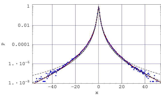
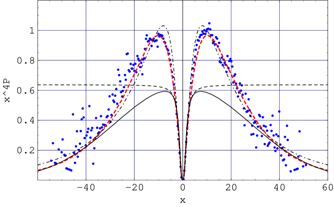
Figure 1: Top panel: lin-log plot of fluid particle acceleration probability density functions, the stretched exponential fit (1) (thick dashed line), the chi-square model (2) (dashed line, $q=3/2$), the log-normal model (3) (dot-dashed line, $s^{2}=3$), and the chi-square Gaussian model (5) (solid line, $q=3/2,a_{c}=39.0$). Bottom panel: the associated contributions to the fourth order moment, $a^{4}P(a)$. Dots: the experimental data points for the transverse (with respect to the large-scale symmetry axis of the studied flow) component of acceleration measured by Crawford, Mordant, and Bodenschatz [4] ($R_{\lambda}=690$, the acceleration is low-pass filtered at 0.23$\tau_{\eta}$ with Gaussian kernel). $x=a/\langle a^{2}\rangle^{1/2}$ denotes normalized Lagrangian acceleration.

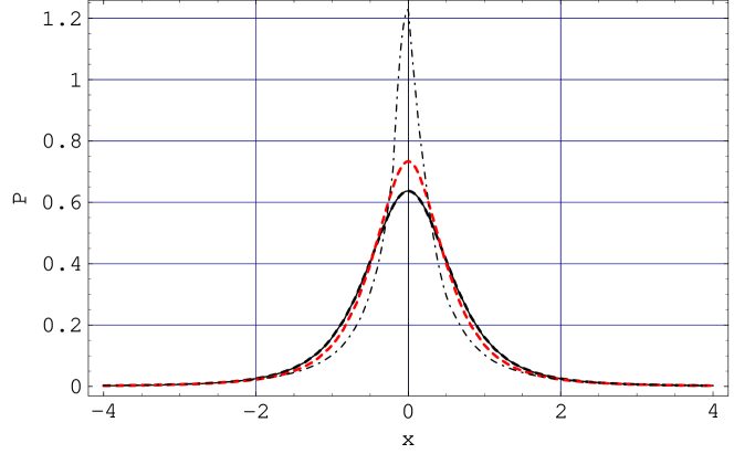
Figure 2: Lin-lin plot of fluid particle acceleration probability density functions. Same notation as in Figure 1.

Actually, one can represent the fluctuating energy dissipation rate as $\epsilon=\bar{\epsilon}+\delta\epsilon$, with $\langle\epsilon\rangle\equiv\bar{\epsilon}\not=0$ and zero mean of the random fluctuating part, $\langle\delta\epsilon\rangle=0$. In the experiments [3], the measured mean energy dissipation rate $\bar{\epsilon}$ varies by about 5 orders of magnitude, from 9.01$\times$10^-5 to 9.16 m${}^{2}\cdot$s^-3, with $R_{\lambda}$ increasing from 140 to 970. Also, the variance of $\delta\epsilon$ varies with approaching to the Kolmogorov scale. Hence, both the effects should be taken into account.

We remind that the basic assumption of the model, $\beta\propto\epsilon_{r}\tau$, used in reference [1] implies that $\beta\propto u_{1}^{2}+u_{2}^{2}+u_{3}^{2}$ at Kolmogorov scale so that $\beta$ is evidently $\chi^{2}$ distributed since the components of velocity fluctuations, $u_{i}$, are known to be approximately normally distributed with zero mean in accord to the experiments [3]. This consideration is partially justified from turbulence dynamics as the acceleration is generally associated to small scales of the flow. The parameter $q$ entering equations (2) and (5) acquires the value $q=(n+3)/(n+1)=3/2$, for the case of a linear drift force, since there are $n=3$ independent random variables $u_{i}$ [1]. It should be emphasized that here $\beta$ is responsible only for a fluctuating part of the energy dissipation.

Immediate testable consequences of the present model are the probability density function $P(a)$ given by equation (5) and the contribution to the fourth order moment, $a^{4}P(a)$. The recent experimental data [4] established a finiteness of the fourth order moment of the component of acceleration, $\langle a^{4}\rangle$.

Plots of the distributions (1)-(3), (5), and the resulting $a^{4}P(a)$ normalized to unit variance are shown in Figures 1 and 2. The numerical value $a_{c}=39.0$ is obtained by a direct fitting of the probability density function (5) to the experimental data [4]. It is due to well overlapping with the data points $P(a)$. Sensitivity of the fitting is of an exponential type.

As one can see from the top panel of Figure 1, the log-normal model (3) (dot-dashed line) provides a good fit to the experimental curve (thick dashed line) in the entire range while the chi-square model (2) (dashed line) and the chi-square Gaussian model (5) (solid line) are in a good qualitative agreement with it except for that the chi-square model implies increasing deviation at big $|a|$. From this point of view, introducing of some truncation of the power law tails and associated additional parameter is a necessary step to provide consistency of the chi-square model with the experiment.

However, the central part of the distributions shown in Figure 2 reveals greater inaccuracy of the log-normal model ($P(0)\simeq 1.23$) as compared with that of both the chi-square and chi-square Gaussian models ($P(0)\simeq 0.65$) which are almost not distinguishable in the region $|a|/\langle a^{2}\rangle^{1/2}\leq 4$; see also recent work by Gotoh and Kraichnan [18]. This is the main failing of the log-normal model (3) for $s^{2}=3.0$ although the predicted distribution follows the measured low probability tails, which are related to the Lagrangian intermittency, to a good accuracy. The central region of the experimental curve (1) ($P(0)\simeq 0.73$) contains most weight of the experimental distribution and is the most accurate part of it, with the relative uncertainty of about 3% for $|a|/\langle a^{2}\rangle^{1/2}<10$ and more than 40% for $|a|/\langle a^{2}\rangle^{1/2}>40$ [17].

It should be noted that both the distributions (3) and (5) show good agreement of $a^{4}P(a)$ (the contribution to the kurtosis summarizing the peakedness of distribution) for small and big $|a|$ but deviate from the experimental data for intermediate $|a|$. This can be readily seen from the heights of the peaks and from their positions in the bottom panel of figure 1, $a/\langle a^{2}\rangle^{1/2}\simeq\pm 8.0$ and $\pm 7.1$ for maximal values of $a^{4}P(a)$ derived from equations (3) and (5), respectively, at the given values of the parameters, as compared to $\pm 10.2$ for the experimental curve (1). Also, in contrast to the chi-square model (2), the chi-square Gaussian model (5) of the present work yields a correct (decaying) behavior of the contribution to kurtosis at big $|a|$ owing to the Gaussian truncation.

4 Conclusions

(i) We have proposed a simple natural extension of the chi-square distribution based stochastic model of fluid particle acceleration in the developed turbulent flow which is found to be characterized by the Gaussian truncated power-law type stationary probability density function of the component of Lagrangian acceleration. Despite one more parameter, $a_{c}$, has been invoked, such a truncation and associated introducing of a new parameter is viewed as a necessary step to provide consistency of implications of the chi-square type model with the observed shape of low-probability tails, which essentially characterize Lagrangian intermittency.

(ii) We have made a comparison of the resulting distribution with that of the chi-square model and the recently proposed log-normal distribution based model. All these models fit the experimental curve $P(a)$ for the transverse component of acceleration to a more or less accuracy (the top panel of Figure 1). However, the contribution to the fourth order moment of acceleration was found to qualitatively discriminate among the models (the bottom panel of Figure 1): the chi-square model gives a qualitatively unsatisfactory behavior of the tails of predicted contribution to kurtosis, $a^{4}P(a)$, while the chi-square Gaussian model provides a good fit only for small ($|a|/\langle a^{2}\rangle^{1/2}<4$) and big ($|a|/\langle a^{2}\rangle^{1/2}>30$) acceleration magnitude values. We found that the Gaussian truncated power law tails are consistent with the observed asymptotics of the acceleration probability density function up to $|a|/\langle a^{2}\rangle^{1/2}=60$. The log-normal model with $s^{2}=3$ meets the experimental data on acceleration distribution in the entire range of measured accelerations but implies a drastically bigger departure from the experimental data in the central region (Figure 2), $|a|/\langle a^{2}\rangle^{1/2}\leq 4$, which represents the most accurate part and the most weight of the measured distribution. Also, both the log-normal and the chi-square Gaussian model do not meet heights and positions of the peaks of the experimental curve $a^{4}P(a)$.

(iii) The considered one-dimensional toy models of the Lagrangian particle acceleration represent explicit examples of parametrization that could be used as prototypical models. Clearly, the choice of relevant forms of the distribution of the parameter $\beta$ is phenomenological but this approach allows one to deal with a part of statistics of complex temporal behavior of fluid particle acceleration in the developed turbulent flow.

The problem of selecting of the underlying distribution of the parameter $\beta$ has been addressed in the recent work [19], in which we related this class of models to the Heisenberg-Yaglom picture of the developed turbulence and constructed the framework which incorporates the log-normal and chi-square Gaussian models in a unified way as particular cases, with the dependence $\beta(u)$ required to be a (monotonic) Borel function of the stochastic Lagrangian velocity fluctuations $u$.

(iv) It should be noted that the gamma (chi-square) distribution of the inverse temperature parameter has been considered from various aspects [1, 20, 21], is known to be in correspondence with a nonlinear Langevin equation for fluctuating temperature appearing in the Landau-Lifschitz theory of fluid fluctuations [22], and shown to be of a universal character for small fluctuations [23]. However, due to the analysis made in the present paper some different distributions of intensive fluctuating parameters [21, 23, 8] appear to be relevant to describe the experimental statistics of fluid particle acceleration in the developed turbulence. In the absence of a direct support from the Navier-Stokes equation, the found departures from the experimental data can also be due to shortcomings of the considered simple class of one-dimensional stochastic models. Thus, it is appropriate to use a more general stochastic approach, such as that with an inclusion of multiplicative noise and nonlinear terms [13], that evidently would require several free parameters to be used.

We conclude by a few remarks.

We note that as it is common to Langevin statistical models of developed turbulence, the considered class of models differs from the phenomenological dimensional analysis (scaling relations) approach since the former is based on a stochastic dynamical framework dealing with time evolution of the Lagrangian acceleration.

Since the introduced parameter $a_{c}$ at fixed $\beta_{0}$ measures variance of the acceleration, equation (8), and the Kolmogorov constant $a_{0}\propto R_{\lambda}^{0.14}$ for high $R_{\lambda}$ [3], the former may depend on the Reynolds number. This dependence could be used to explain the fact that the experimental $P(a)$ was found to have Reynolds number dependent stretched exponential tails [3].

References

- [1] Beck C 2001 Phys. Rev. Lett. 87 180601; Beck C 2001 Generalized statistical mechanics and fully developed turbulence Preprint cond-mat/0110073
- [2] Tsallis C 1988 J. Stat. Phys. 52 479
- [3] La Porta A, Voth G A, Crawford A M , Alexander J, and Bodenschatz E 2001 Nature 409 1017; Voth G A , La Porta A, Crawford A M, Bodenschatz E, Alexander J 2002 J. Fluid Mech. 469 121 (Voth G A, La Porta A, Crawford A M, Bodenschatz E, and Alexander J 2001 Measurement of particle accelerations in fully developed turbulence Preprint physics/0110027)
- [4] Crawford A M, Mordant N, Bodenschatz E, and Reynolds A M 2002 Comment on ”Dynamical foundations of nonextensive statistical mechanics” Preprint physics/0212080, submitted to Phys. Rev. Lett.
- [5] Beck C 2000 Physica A 277 115; 2001 Phys. Lett. A 287 240; 2002 Europhys. Lett. 57 329; 2001 Non-additivity of Tsallis entropies and fluctuations of temperature Preprint cond-mat/0105371
- [6] Wilk G and Wlodarczyk Z 2000 Phys. Rev. Lett. 84 2770
- [7] Sawford B L 1991 Phys. Fluids A 3 1577; Pope S B 2002 Phys. Fluids 14 2360
- [8] Beck C 2002 Lagrangian acceleration statistics in turbulent flow Preprint cond-mat/0212566
- [9] Reynolds A M 2003 Phys. Fluids 15 L1; Phys. Rev. Lett. 91 084503
- [10] Renner Ch, Peinke J, and Friedrich R 2002 On the interaction between velocity increment and energy dissipation in the turbulent cascade, Preprint physics/0211121; Renner Ch, Peinke J, Friedrich R, Chanal O, and Chabaud B 2002 Phys. Rev. Lett. 89 124502; Friedrich R 2003 Phys. Rev. Lett. 90 084501
- [11] Mordant N, Delour J, Leveque E, Arneodo A, and Pinton J-F 2002 Phys. Rev. Lett. 89 254502; Mordant N, Delour J, Leveque E, Arneodo A, and Pinton J-F 2002 Long time correlations in Lagrangian dynamics: a key to intermittency in turbulence Preprint physics/0206013
- [12] Castaing B, Gagne Y, and Hopfinger E J 1990 Physica D 46 177
- [13] Laval J-P, Dubrulle B, and Nazarenko S 2001 Phys. Fluids 13 1995 (Laval J-P, Dubrulle B, and Nazarenko S 2001 Non-locality and intermittency in 3D turbulence Preprint physics/0101036)
- [14] Kraichnan R H and Gotoh T 2002 data presented at the workshop on Anomalous Distributions, Nonlinear Dynamics, and Nonextensity, Santa Fe, November 2002
- [15] Tsallis C and Souza A M C 2002 Constructing a statistical mechanics for Beck-Cohen superstatistics Preprint cond-mat/0206044
- [16] Aringazin A K and Mazhitov M I 2002 Phenomenological Gaussian screening in the nonextensive statistics approach to fully developed turbulence Preprint cond-mat/0212462.
- [17] Mordant N, Crawford A M, and Bodenschatz E 2003 Experimental Lagrangian acceleration probability density function measurement Preprint physics/0303003
- [18] Gotoh T and Kraichnan R H 2003 Turbulence and Tsallis statistics Preprint nlin.CD/0305040
- [19] Aringazin A K and Mazhitov M I 2003 Phys. Lett. A 313 284 (Aringazin A K and Mazhitov M I 2003 The PDF of fluid particle acceleration in turbulent flow with underlying normal distribution of velocity fluctuations Preprint cond-mat/0301245)
- [20] Johal R 1999 An interpretation of Tsallis statistics based on polydispersity Preprint cond-mat/9909389
- [21] Aringazin A K and Mazhitov M I 2003 Physica A 325 409 (Aringazin A K and Mazhitov M I 2002 Quasicanonical Gibbs distribution and Tsallis nonextensive statistics Preprint cond-mat/0204359)
- [22] Bashkirov A G and Sukhanov A D 2002 Zh. Eksp. Teor. Fiz. (Russian JETP) 95 440
- [23] Beck C and Cohen E G D 2003 Physica A 322 267 (Beck C and Cohen E G D 2002 Superstatistics Preprint cond-mat/0205097)