Band structure, elementary excitations, and stability of a Bose-Einstein condensate in a periodic potential

Abstract

We investigate the band structure of a Bose-Einstein condensate in a one-dimensional periodic potential by calculating stationary solutions of the Gross-Pitaevskii equation which have the form of Bloch waves. We demonstrate that loops (“swallow tails”) in the band structure occur both at the Brillouin zone boundary and at the center of the zone, and they are therefore a generic feature. A physical interpretation of the swallow tails in terms of periodic solitons is given. The linear stability of the solutions is investigated as a function of the strength of the mean-field interaction, the magnitude of the periodic potential, and the wave vector of the condensate. The regions of energetic and dynamical stability are identified by considering the behavior of the Gross-Pitaevskii energy functional for small deviations of the condensate wave function from a stationary state. It is also shown how for long-wavelength disturbances the stability criteria may be obtained within a hydrodynamic approach.

I Introduction

The possibility of studying experimentally the properties of quantum atomic gases in the periodic potential created by interference of two laser beams, a so-called optical lattice, has led to an explosion of activity, both experimental and theoretical. One of the basic properties of an atom moving in a periodic potential is that it undergoes Bloch oscillations when subjected to a sufficiently weak external force. In a gas of thermal cesium atoms such oscillations were observed as long ago as 1996 Ben Dahan et al. (1996). Subsequently, a number of experimental studies of Bose-Einstein condensates in optical lattices have been made. In one-dimensional lattices, interference has been observed between condensates initially trapped in different local minima of the potential Anderson and Kasevich (1998). Also Bloch oscillations Burger et al. (2001) and Josephson oscillations Cataliotti et al. (2001) of a condensate have been observed, and acceleration and collective behavior of a condensate have been studied Morsch et al. (2001). In higher-dimensional lattices, interference effects have been investigated and the transition to an insulating state has been observed Greiner et al. (2002).

On the theoretical side, Bloch oscillations have been investigated Berg-Sørensen and Mølmer (1998), and states of uniform flow have been studied Choi and Niu (1999); Wu and Niu (2000). For sufficiently weak interparticle interaction, the properties of a Bose-Einstein condensate resemble those of a single particle moving in a periodic potential. Properties of a condensate in this regime have been explored in Ref. Wu and Niu (2001). One of the surprising discoveries is that the interaction between particles can influence the band structure dramatically. In a two-state model, Wu and Niu found a loop in the band structure at the boundary of the first Brillouin zone Wu and Niu (2000) and, in detailed calculations of band structure, Wu et al. found evidence for non-analytic behavior at the zone boundary Wu et al. (2002). Another unexpected discovery was that for sufficiently strong particle interactions, there exists a simple exact solution to the Gross-Pitaevskii equation for a condensate with a wave vector $k$ corresponding to the boundary of the first Brillouin zone Bronski et al. (2001a, b). More recently Diakonov et al. have carried out explicit numerical calculations of the band structure, and have demonstrated that the band has a swallow-tail feature at the zone boundary Diakonov et al. (2002). They also showed that this behavior is predicted by the simple two-component model used previously by Wu and Niu Wu and Niu (2000).

One purpose of this article is to calculate properties of stationary states of a Bose-Einstein condensate in an optical lattice. We carry out numerical calculations of the band structure and investigate the size of the loop at the boundary of the first Brillouin zone. In addition, it is demonstrated that a similar swallow-tail structure can arise at the zone center. It is remarkable that the width of the swallow tails remains nonzero even in the absence of the lattice potential. We show how this may be understood in terms of periodic solitons which, for the Gross-Pitaevskii equation, were first investigated by Tsuzuki Tsuzuki (1971).

A second purpose of the paper is to explore elementary excitations and stability of states of uniform superflow. For relatively weak interparticle interactions, this has been done in Refs. Wu and Niu (2000) and Wu and Niu (2001), and we shall in this paper devote most attention to the range of parameters for which there are loops in the band structure. Quite generally, linear stability of states may be investigated by expanding the Gross-Pitaevskii energy functional to second order in the deviation of the condensate wave function from the solution for a stationary state. One may distinguish two types of stability. The first is energetic stability, which is referred to in Ref. Wu and Niu (2001) as “Landau stability”, and the condition for this is that the changes in the Gross-Pitaevskii energy functional due to the change in the condensate wave function be positive definite. The other form of stability is dynamical stability, and the criterion for this is that the linearized time-dependent Gross-Pitaevskii equation have no complex eigenvalues. To describe excitations with wavelengths long compared with the period of the lattice, a hydrodynamic approach may be applied. This work represents a generalization to moving condensates of the calculations of Ref. Krämer et al. (2002) for condensates at rest. It yields a stability criterion for creation of long-wavelength phonons which reduces for a translationally-invariant system to the Landau criterion.

The results obtained in this work are derived from numerical solutions to the one-dimensional Gross-Pitaevskii equation. The method we adopt is to expand the wave function in a Fourier series. In order to elucidate the physical meaning of our results, we have also carried out approximate analytic calculations which yield simple results in qualitative agreement with those of the numerical calculations.

In this paper we shall consider only extended states having the form of Bloch waves. Due to the nonlinear nature of the Gross-Pitaevskii equation there are also stationary states corresponding to localized excitations such as isolated solitons Trombettoni and Smerzi (2001), as well as states in which the density varies periodically with a period different from that of the optical potential.

This paper is organized as follows. In Sec. II the properties of stationary states are described. There we present analytical and numerical calculations, and describe how swallow-tail structures may be understood in terms of periodic solitons. Section III gives a general discussion of elementary excitations of a condensate, and energetic and dynamical stability. It describes the hydrodynamic approach applicable at long wavelengths. Numerical results for the stability of a condensate in a one-dimensional optical lattice are given in Sec. IV. Section V contains a discussion of our results and concluding remarks.

II Bloch waves

The basic assumption that we shall make in this paper is that fluctuation effects are so small that the state of the condensate may be calculated in the Gross-Pitaevskii approach, in terms of the condensate wave function $\psi({\bf r})$. The energy of the state is then given by

$$E[\psi]=\int d{\bf r}\left(\frac{\hbar^{2}}{2m}|\boldsymbol{\nabla}\psi|^{2}+V({\bf r})|\psi|^{2}+\frac{1}{2}U_{0}|\psi|^{4}\right).$$

(1)

Here $m$ is the mass of a particle, $V({\bf r})$ is the external potential and $U_{0}$ is the effective interaction between two atoms, which is given in terms of the scattering length $a$ for two-body collisions by $U_{0}=4\pi\hbar^{2}a/m$.

Stationary states of the condensate may be found in the usual way by demanding that the energy functional (1) be stationary under variations of $\psi({\bf r})$, subject to the condition that the total number of particles remain unchanged. This yields the time-independent Gross-Pitaevskii equation

$$-\frac{\hbar^{2}}{2m}\nabla^{2}\psi+V({\bf r})\psi+U_{0}|\psi|^{2}\psi=\mu\psi,$$ (2)

where $\mu$ is the chemical potential.

A one-dimensional optical lattice gives rise to a potential acting on an atom which has the form

$$V(x)=2V_{0}\cos^{2}(\pi x/d)=V_{0}\cos(2\pi x/d)+V_{0},$$ (3)

where $d$ is the period of the lattice. The coefficient $V_{0}$, which measures the strength of the potential, depends on the polarizability of the atom and the intensity of the radiation that generates the optical lattice. In future we shall generally neglect the constant term, and take the potential to be simply $V_{0}\cos(2\pi x/d)$ . In addition, we shall not take the potential due to the trap into account. Such an approach should give a good approximation to the local properties of stationary states of the condensate, provided the average density and average wave number of the condensate vary slowly in space on the scale of the period of the optical lattice. For studying excitations, this approach will be valid provided the wavelength of the excitations is large compared with the lattice spacing but small compared with the distance over which properties of the unperturbed condensate vary significantly. A further assumption we shall make is that the states are uniform in the $y$ and $z$ directions. The resulting Gross-Pitaevskii equation has a variety of different sorts of stationary solution. Some of these are extended, while others, such as solitons, are localized in space. In this paper we shall focus on extended solutions to Eq. (2). These are the analogs of Bloch states for a single particle in a lattice. As remarked in the introduction, there are stationary solutions of the Gross-Pitaevskii equation for which the particle density does not have the same period as the lattice. As will be explained elsewhere, they are related to the self-trapped states of a condensate in a double-well potential Milburn et al. (1997); Smerzi et al. (1997); Coullet and Vandenberghe (2002); Mahmud et al. (2002). Here we shall confine our attention to solutions of the usual Bloch form

$$\psi(x)={\rm e}^{ikx}f(x),$$ (4)

where $\hbar k$ is the quasimomentum and $f(x)$ has the same period as the lattice, $f(x)=f(x+d)$.

The energy per unit volume, ${\tilde{E}}$, is then given by

$${\tilde{E}} = \frac{1}{d}\int_{-d/2}^{d/2}dx\left[\frac{\hbar^{2}}{2m}\left|\frac{d\psi}{dx}\right|^{2}\right.$$ (5)

$$\left.+V_{0}\cos\left(\frac{2\pi x}{d}\right)|\psi|^{2}+\frac{1}{2}U_{0}|\psi|^{4}\right].$$

We determine equilibrium solutions $\psi$ of the time-independent Gross-Pitaevskii equation by expanding $\psi$ in plane waves,

$$\psi_{k}=\sqrt{n}{\rm e}^{ikx}\sum^{\nu_{\rm max}}_{\nu=-\nu_{\rm max}}{a_{\nu}{\rm e}^{i2\pi\nu x/d}},$$ (6)

where $\nu$ is an integer. Here

$$n=\frac{1}{d}\int_{-d/2}^{d/2}dx|\psi|^{2}$$ (7)

is the average particle density. From this it follows that the coefficients $a_{\nu}$ satisfy the normalization condition

$$\sum^{\nu_{\rm max}}_{\nu=-\nu_{\rm max}}|a_{\nu}|^{2}=1.$$ (8)

The stationary states of the system may be obtained by a variational method, by requiring that the derivatives of the energy functional (5) with respect to $a_{\nu}$ vanish. There are $2\nu_{\rm max}+1$ complex variables, and one real constraint (8). In addition, the overall phase of the wave function is arbitrary, so the energy functional depends on $4\nu_{\rm max}$ independent real variables.

A considerable simplification of the computational effort is possible because it turns out that for the stationary states of interest for the range of parameters we have considered, the phases $\phi_{\nu}$ of the coefficients $a_{\nu}$ may be taken to be the same, or to differ by $\pi$. It is easy to demonstrate that such states are indeed stationary under variations of the phases because the phases occur in the energy functional as terms of the type $\cos(\phi_{\nu_{1}}-\phi_{\nu_{2}})$ and $\cos(\phi_{\nu_{1}}+\phi_{\nu_{2}}-\phi_{\nu_{3}}-\phi_{\nu_{4}})$. The derivatives of these functions with respect to the phases thus give terms of the type $\sin(\phi_{\nu_{1}}-\phi_{\nu_{2}})$ and $\sin(\phi_{\nu_{1}}+\phi_{\nu_{2}}-\phi_{\nu_{3}}-\phi_{\nu_{4}})$, which vanish if the phases are zero or $\pi$. We sought solutions with other phases by allowing the coefficients to be complex, but found none. Because the overall phase is arbitrary, this means that we may take the $a_{\nu}$ to be real. When this is done, there are only $2\nu_{\rm max}$ independent real variables.

We shall present our results in terms of the energy per particle, ${\tilde{E}}/n$, as a function of the (one-dimensional) wave vector $k$. As a convenient unit of energy we employ the quantity $E_{0}$ given by

$$E_{0}=\frac{\hbar^{2}\pi^{2}}{2md^{2}},$$ (9)

which is the kinetic energy of a particle with wave vector equal to that at the boundary of the first Brillouin zone. For an optical lattice made by oppositely directed laser beams, the lattice spacing is half the wavelength $\lambda$ of the light, and therefore $E_{0}$ is equal to the kinetic energy given to an atom initially at rest when it absorbs a photon having the frequency of the laser.

An unusual feature of the resulting energy bands is the appearance of loops in the form of swallow-tail structures, as demonstrated in Ref. Diakonov et al. (2002). One noteworthy result of the present work is that swallow tails can occur also at the zone center in higher-lying bands, as illustrated in Fig. 1, which shows results of numerical calculations of the band structure that will be described in Sec. II.2. Thus the appearance of swallow tails is a general feature. At the zone boundary, the swallow tail appears when the interaction energy per particle $nU_{0}$ exceeds the amplitude $V_{0}$ of the potential due to the optical lattice. As the parameter $nU_{0}$ grows with respect to $V_{0}$, the swallow tail increases in width and may extend deep into the zone. The condition $nU_{0}>V_{0}$ is necessary for the swallow-tail structure to appear at the zone boundary, $k=\pi/d$.

Had swallow tails appeared only at the zone boundary, one might have suspected that their existence was related to the fact that for $k=\pi/d$ there is an exact solution to the Gross-Pitaevskii equation. However, for $k=0$ there is no exact solution of the Gross-Pitaevskii equation, and consequently the existence of swallow tails is not connected with the existence of an exact solution. As we shall see in detail below, the condition for the appearance of a loop at the zone center can be much less restrictive than at the zone boundary. Before discussing our numerical results further, we shall now analyze a simple model for the band structure near the zone center which exhibits the main qualitative features of the full numerical calculations.

II.1 An analytic model

In Ref. Diakonov et al. (2002) the swallow-tail structure of the lowest energy band at the boundary of the first Brillouin zone was discussed in terms of a simple trial solution to the Gross-Pitaevskii equation. In order to illustrate the generic nature of the phenomenon we shall here consider the band structure at the center of the Brillouin zone, corresponding to $k=0$.

We employ a trial function of the form

$$\psi=\sqrt{n}{\rm e}^{ikx}(a_{0}+a_{1}{\rm e}^{i2\pi x/d}+a_{-1}{\rm e}^{-i2\pi x/d}),$$ (10)

where the coefficients $a_{0}$, $a_{1}$ and $a_{-1}$ are chosen to be real for the reasons given above. The trial function thus mixes into the free-particle wave function $\exp(ikx)$ states that differ by the smallest reciprocal lattice vectors, $\pm 2\pi/d$. The normalization condition (8) is

$$a_{0}^{2}+a_{1}^{2}+a_{-1}^{2}=1.$$ (11)

This constraint is satisfied automatically by expressing the coefficients in terms of two angles $\theta$ and $\phi$ according to the equations

$$a_{0}=\cos\theta,\;\;a_{1}=\sin\theta\cos\phi,\;\;{\rm and}\;\;\;\;a_{-1}=\sin\theta\sin\phi.$$ (12)

Upon inserting the trial function (10) with coefficients given by Eq. (12) into Eq. (5), we obtain

$$\frac{{\tilde{E}}}{n}=\epsilon_{\rm kin}+\epsilon_{\rm pot}+\epsilon_{\rm int},$$ (13)

where

$$\epsilon_{\rm kin}=\frac{\hbar^{2}}{2m}\left[k^{2}+2k\left(\frac{2\pi}{d}\right)\sin^{2}\theta(\cos^{2}\phi-\sin^{2}\phi)\right.$$

$$\left.+\left(\frac{2\pi}{d}\right)^{2}\sin^{2}\theta\right]$$ (14)

is the kinetic energy,

$$\epsilon_{\rm pot}=V_{0}\sin\theta\cos\theta(\cos\phi+\sin\phi)$$ (15)

is the potential energy, and

$$\epsilon_{\rm int}=nU_{0}\left(\frac{1}{2}+\cos^{2}\theta\sin^{2}\theta(\cos\phi+\sin\phi)^{2}\right.$$

$$+\left.\frac{1}{4}\sin^{4}\theta\sin^{2}2\phi\right)$$ (16)

is the interaction energy. The stationary points of this energy function are obtained by equating to zero the derivatives of the energy per particle with respect to $\theta$ and $\phi$. The results shown in Fig. 2 were found with this model.

Figure 1: Energy per particle as a function of wave number for the lowest bands. The results are obtained from numerical calculations based on the wave function (6), as described in Sec. II.2.

Figure 2: Model calculations of the energy per particle as a function of wave number for the same parameters as were used in Fig 1. The results are obtained using the variational method with the trial function (10).

In order to exhibit the nature of the solutions, we first consider the simple case in the absence of interactions ($U_{0}=0$), and with $V_{0}\ll E_{0}$, so the lattice potential is a small perturbation. At $k=0$ one finds three stationary points with different energies. The lowest state corresponds to the bottom of the lowest band, and its wave function is a plane wave with $k=0$ plus a small admixture of states with $k=\pm 2\pi/d$. Its energy is given to second order in $V_{0}$ by $E=-(V_{0})^{2}/8E_{0}$. The two other states are comprised primarily of plane waves with $k=\pm 2\pi/d$ with a small admixture of the $k=0$ state. The energies of the two states are $E=4E_{0}$ for the state which corresponds to the top of the second band, and $E=4E_{0}+(V_{0})^{2}/8E_{0}$ for the state at the bottom of the third band. Because of the simplicity of the trial function, there are no higher bands in this model. The magnitude of the energy gap at $k=0$ between the second and third bands is thus $V_{0}^{2}/8E_{0}$. The reason that it is of second order in the lattice potential is that the potential is sinusoidal with period $d$. Consequently, it couples directly only states with wave numbers differing by the smallest reciprocal lattice vectors, $\pm 2\pi/d$. The coupling between states with wave vectors $k+2\pi/d$ and $k-2\pi/d$ is indirect, since it is brought about by the coupling of these states to the state with wave vector $k$. In the absence of interactions between particles, the stationary points of the energy functional for $k=0$ have $|a_{1}|=|a_{-1}|$, that is $\phi$ is an odd multiple of $\pi/4$.

Figure 3a shows results for non-interacting particles ($U_{0}=0$). The familiar band structure is seen. The band gap is $V_{0}$ at $k=\pi/d$ and $V_{0}^{2}/8E_{0}$ at $k=0$ for small $V_{0}$, which is still a good approximation at $V_{0}=2E_{0}$. The lowest band is pushed down in the presence of the periodic potential .

In the presence of interactions ($U_{0}\neq 0$), the energy landscape in the $\theta$-$\phi$ plane has a more complicated structure, and the number of points at which the energy functional is stationary can be greater than for $U_{0}=0$. Figure 3b exhibits the resulting band structure. The band gap at $k=0$ is enhanced by the interaction, in contrast to the band gap at $k=\pi/d$, which is reduced.

Let us now examine the behavior of the band structure in the limit of vanishing lattice potential ($V_{0}\rightarrow 0$). As one would expect, the band gaps tend to zero while, in contrast, the widths of swallow tails increase with decreasing $V_{0}$, and they are nonzero for $V_{0}\rightarrow 0$. In this limit, states corresponding to the upper edge of a swallow tail become degenerate with states in the band above. As we shall discuss in Sec. II.3, the reason for this surprising behavior is that states on the upper edge of a swallow tail correspond to periodic soliton solutions of the Gross-Pitaevskii equation.

The appearance of a swallow tail requires that the interaction energy $nU_{0}$ be sufficiently large. In the calculations for states near the zone boundary in Ref. Diakonov et al. (2002), it was shown that the condition for existence of the swallow tail is $nU_{0}>V_{0}$. We now carry out a similar calculation for the swallow tail at the zone center, using the three-state model described above. We investigate the form of the energy function (13–16) for $k=0$ near the point $\theta=\pi/2$, $\phi=3\pi/4$. This is a stationary point both for $U_{0}=0$ and for $U_{0}\neq 0$. If one imagines that $U_{0}$ increases gradually from zero while the other parameters remain fixed, one observes in the energy landscape given by (13–16) that two additional stationary points are split off from $(\theta,\phi)=(\pi/2,3\pi/4)$ when $nU_{0}$ exceeds a critical value. This value may be found by inserting $\theta=\pi/2+\delta$ and $\phi=3\pi/4+\epsilon$ into Eqs. (13–16) and expanding the energy to second order in $\delta$ and $\epsilon$. The resulting expression for the change in the energy per particle relative to its value for $\delta=\epsilon=0$ is

$$\frac{{\tilde{E}}}{n}-4E_{0}-\frac{3}{4}nU_{0}\simeq-4E_{0}\delta^{2}+\sqrt{2}V_{0}\delta\epsilon-\frac{nU_{0}}{2}(\delta^{2}+2\epsilon^{2}).$$ (17)

For $nU_{0}=0$, the point $\delta=\epsilon=0$ is a saddle point. As $nU_{0}$ increases, this point turns into a local maximum, and two saddle points move out to points with both $\delta$ and $\epsilon$ nonzero. The condition for the saddle point to turn into a local maximum is that the symmetric matrix yielding the quadratic form (17) have a zero eigenvalue, and this occurs for $nU_{0}(nU_{0}+8E_{0})=V_{0}^{2}$ or

$$nU_{0}=[(4E_{0})^{2}+V_{0}^{2}]^{1/2}-4E_{0}.$$ (18)

For values of the lattice potential small compared with $E_{0}$, ($V_{0}\ll E_{0}$), the critical value obtained from Eq. (18) becomes $nU_{0}=V_{0}^{2}/8E_{0}$. This is physically reasonable, since the magnitude of the energy gap in the absence of interactions equals $V_{0}^{2}/8E_{0}$, as discussed above. At the zone boundary, however, the energy gap in the absence of interactions is equal to $V_{0}$, corresponding to the condition $nU_{0}>V_{0}$ for the appearance of the swallow-tail structure at $k=\pi/d$. Note that the result (18) is derived from an approximate trial function which becomes exact only in the limit $V_{0}\ll E_{0}$. Even so, it yields a reasonable description of the dependence of the critical value of $nU_{0}$ on $V_{0}$ also for higher values of $V_{0}$, as shown by the numerical results for the width of the swallow tail in Fig. 5 below.

Figure 3: Energy per particle in the first Brillouin zone as in Fig 2. The results are obtained by a variational method with the trial function given in Eq. (10). a) In the absence of interaction the band structure (bold curves) exhibits the usual band gaps at $k=0$ and $k=\pi/d$. The band gap is $V_{0}$ at $k=\pi/d$ and $V_{0}^{2}/8E_{0}$ at $k=0$ for small $V_{0}$. The thin curves show the energies for $V_{0}\rightarrow 0$, i.e. for the free non-interacting system. b) In the presence of interaction the swallow tails appear for $U_{0}$ larger than a critical value, which depends on $V_{0}$ and is different for the two band gaps (bold curves). The thin curves illustrate the limit $V_{0}\rightarrow 0$.

The swallow-tail structure illustrated in Figs. 1-3 is thus a general phenomenon, in that it occurs both at the zone boundary and at the zone center, provided the interaction energy $nU_{0}$ is sufficiently large. The phenomenon also occurs at other points in the Brillouin zone for solutions which have a periodicity different from that of the optical lattice, as will be demonstrated in future work.

II.2 Numerical calculations of band structure

At the beginning of this section we described the general method used to calculate stationary states of a moving condensate. Our numerical procedure is as follows: The trial function (6) is inserted into the energy functional (5), and stationary points of the resulting expression for the energy are found. The normalization of the wave function is imposed as in Eq. (8), or by generalizing Eq. (12) to hyperspherical coordinates. We determine the solutions by using the Mathematica^® routine “FindRoot”, which requires as input an initial guess for the solution. The latter is found by first solving the problem in a reduced basis. Once a solution has been found for a particular value of $k$, this is used as the initial guess for nearby values of $k$.

In Fig. 1 two examples of numerical results for the band structure are presented. The results are calculated with $\nu_{\rm max}=4$. This corresponds to a number of basis functions equal to $2\nu_{\rm max}+1$. The results for $\nu_{\rm max}=4$ and $\nu_{\rm max}=5$ differ by less than the thickness of the lines. Around $k=\pi/d$ the energy of the second band calculated with $\nu_{\rm max}=2$ differs by less than 1% from the full numerical result. Around $k=0$ and for higher bands, more plane waves contribute, and typically $\nu_{\rm max}=3$ is needed for 1% convergence. Compared to the simple model used in Fig. 2, the numerical results exhibit smaller swallow tails. The higher-lying energy bands are shifted downwards more than the lower-lying ones, causing the band gaps to become narrower.

Rather than exhibiting the full band structure for different choices of the parameters, we choose to illustrate how one particular feature, the widths of the swallow tails at the zone boundary and at the zone center, depends on the two dimensionless quantities in the problem, $nU_{0}/E_{0}$ and $V_{0}/E_{0}$. If the band structure is displayed in the reduced zone scheme, a swallow tail may be split up into a number of segments. This is shown in Figs. 1-3, where the swallow tail at the zone boundary is divided into two halves. The full swallow tail may be seen in an extended zone representation, and we define the width $w$ of a swallow tail as being the magnitude of the difference between the values of $k$ at the two tips of a swallow tail in this representation. Widths of swallow tails are exhibited as contour plots in Fig. 4 and Fig. 5.

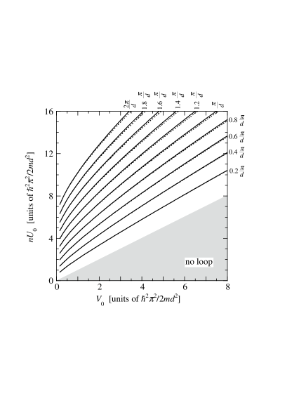
Figure 4: Contour plot of the width of the swallow tail in the lowest band around $k=\pi/d$. The shaded area indicates the region where the swallow tail is absent, i.e., for $nU_{0}<V_{0}$.

In Fig. 4 we show a contour plot of the width of the swallow tail at the zone boundary in the first band as a function of the mean-field interaction $nU_{0}$ and the potential parameter $V_{0}$. The full lines are obtained from numerical solutions with $\nu_{\rm max}=3$, which is sufficiently large to ensure an accuracy better than the thickness of the lines. The dotted lines are results for $\nu_{\rm max}=2$.

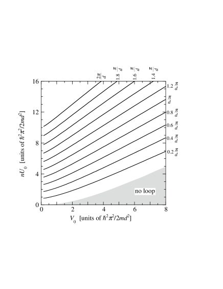
Figure 5: Contour plot of the width of the swallow tail in the second band around $k=0$. If the condensate wave function is approximated by the truncated expression (10), this swallow tail is absent if the mean field interaction is less than a critical value given by Eq. (18). The corresponding region in parameter space is indicated by the shaded area.

The analytic model using the trial function (10) overestimates the width by less than 50% for $nU_{0}<8E_{0}$ and $V_{0}<8E_{0}$. Table 1 shows examples of calculated widths for different basis sizes. We denote the widths calculated for a particular value of $\nu_{\rm max}$ by $w_{\nu_{\rm max}}$. In all cases, inclusion of more plane waves improves the result. The precision is dependent mainly on the width. Around $k=\pi/d$, fewer plane waves are needed than around $k=0$ to describe the wave function to a given accuracy, and therefore the precision of the width estimates decreases with increasing width for fixed $\nu_{\rm max}$. Correspondingly, the precision improves with decreasing $nU_{0}$ and increasing $V_{0}$.

Table 1: Dependence on basis size of the calculated width $w_{\nu_{\rm max}}$ of the swallow tail at the zone boundary. The table shows $w_{6}$ in units of $\pi/d$, and the difference $w_{\nu_{\rm max}}/w_{6}-1$ in per cent.

			Difference
$V_{0}$	$nU_{0}$	$w_{6}$	for $\nu_{\rm max}$
			1	2	3
$E_{0}$	$2E_{0}$	0.185547	13.6	0.25	0.00
$E_{0}$	$4E_{0}$	0.675781	27.1	1.05	0.02
$E_{0}$	$8E_{0}$	1.56555	46.7	3.19	0.13
$4E_{0}$	$8E_{0}$	0.552031	35.0	3.50	0.20
$6E_{0}$	$8E_{0}$	0.182891	27.8	2.69	0.13

The width of the swallow tail in the second band around $k=0$ is shown in Fig. 5. As we described in the previous subsection, this swallow tail exists provided $nU_{0}$ exceeds a critical value, which for small values of $V_{0}/E_{0}$ is given by $V_{0}^{2}/8E_{0}$. The analytic model using the trial function (10) estimates the width within 25% for $nU_{0}/E_{0}<8$ and $V_{0}/E_{0}<8$. Table 2 shows some examples of the precision within that parameter range. In this case, the calculated widths using $\nu_{\rm max}=1$ are closer to the full numerical results than are those calculated using $\nu_{\rm max}=2$. For $\nu_{\rm max}>2$ the precision systematically improves. The precision becomes worse as $nU_{0}$ and $V_{0}$ increase.

The asymptotic behavior of the contours in Fig. 5 for $V_{0}\rightarrow 0$ can be determined analytically within the simple model described in Sec. II.1. The thin lines in Fig. 3 show an example of the band structure in this limit. For fixed $nU_{0}$, the width of the swallow tail increases with decreasing $V_{0}$, and it is nonzero for $V_{0}=0$. At the tip of the swallow tail these stationary points of the energy function (13) merge at $(\theta,\phi)=(\pi/2,0)$ for $V_{0}\rightarrow 0$. The interaction energy $\epsilon_{\rm int}$ has a minimum while the kinetic energy $\epsilon_{\rm kin}$ has a maximum at $(\pi/2,0)$. Therefore the stationary points merge when the upward curvature of $\epsilon_{\rm int}$ and the downward curvature of $\epsilon_{\rm kin}$ in the $\phi$-direction cancel at $(\pi/2,0)$:

$$\left.\frac{\partial^{2}}{\partial\phi^{2}}\epsilon_{\rm kin}\right|_{\theta=\pi/2}=-\left.\frac{\partial^{2}}{\partial\phi^{2}}\epsilon_{\rm int}\right|_{\theta=\pi/2}.$$ (19)

From this criterion we obtain the asymptotic width of the swallow tail at the zone center $w=(\pi/4d)nU_{0}/E_{0}$ for $V_{0}\rightarrow 0$. Compared to the numerical result in Fig. 5, this analytic result underestimates the asymptotic value of $nU_{0}$ for $V_{0}\rightarrow 0$ by $7\%$ for $w=0.2\pi/d$, and by $26\%$ for $w=2\pi/d$.

Table 2: Dependence on basis size of the calculated width $w_{\nu_{\rm max}}$ of the swallow tail at the zone center. The table shows $w_{6}$ in units of $\pi/d$, and the difference $w_{\nu_{\rm max}}/w_{6}-1$ in per cent.

			Difference
			for $\nu_{\rm max}$
$V_{0}$	$nU_{0}$	$w_{6}$	1	2	3	4	5
$E_{0}$	$E_{0}$	0.077969	-0.95	4.36	0.05	0.00	0.00
$E_{0}$	$4E_{0}$	0.373789	3.97	13.4	0.16	0.03	0.00
$E_{0}$	$8E_{0}$	0.726953	10.5	24.0	0.36	0.17	0.01
$4E_{0}$	$8E_{0}$	0.432695	0.86	34.0	0.97	0.87	0.06
$8E_{0}$	$8E_{0}$	0.155234	-20.3	68.4	3.32	2.52	0.33

For the swallow tail at the zone boundary, Fig. 4, the analysis is further simplified by taking $\phi=\pi/2$, which is an exact solution at $k=\pi/d$ Bronski et al. (2001a, b). The value $\theta_{0}$ at which the energy is stationary varies continuously around the loop. The tip of the swallow tail is found by setting the derivative of $k$ with respect to $\theta_{0}$ equal to 0. This yields $\sin 2\theta_{0}=-(V_{0}/nU_{0})^{1/3}$, and a width

$$w=\frac{\pi}{2d}\left[\left(\frac{nU_{0}}{E_{0}}\right)^{2/3}-\left(\frac{V_{0}}{E_{0}}\right)^{2/3}\right]^{3/2}.$$ (20)

Compared to the numerical result in Fig. 4 the contours predicted by Eq. (20) are shifted towards lower values of $nU_{0}$, i.e., the width is somewhat overestimated by Eq. (20). For $nU_{0}=2E_{0}$ and $V_{0}=E_{0}$ the width given by Eq. (20) is 21% above the numerical result and, for $nU_{0}=4E_{0}$ and $V_{0}=2E_{0}$, 38% above. The model is thus most precise for small widths.

II.3 Physical understanding of swallow tails

A striking feature of the results above is that the width of the swallow tail is nonzero as the strength of the periodic potential tends to zero. As we shall now describe, the states on the upper edge of the swallow tail then correspond to periodic soliton solutions of the Gross-Pitaevskii equation first discussed for a condensate in the absence of an external potential by Tsuzuki Tsuzuki (1971). For potentials having the form of Jacobi elliptic functions, analytical results for periodic solitons have been obtained in Ref. Bronski et al. (2001b).

The simplest case to think about is that at the zone boundary, $k=\pi/d$. The solution is then an equally spaced array of dark solitons (that is solitons for which the wave function vanishes on some surface), with one soliton per lattice spacing of the periodic potential. That this solution has wave vector $\pi/d$ may be seen from the fact that the phase difference across a dark soliton is $\pi$. Since there is one soliton per lattice spacing, the wave vector $k$, which is the average phase change per unit length, is thus $\pi/d$. For states with this value of the wave vector, the energy of the highest state in the first band and the energy of the state in the second band are degenerate if the lattice potential is absent, but the degeneracy is broken when a weak periodic potential is applied. The state having dark solitons with centers at $x=\tau d$, where $\tau$ is an integer, has a lower energy, since the solitons, which are density rarefactions, are located at the maxima of the lattice potential. On the other hand, the state having solitons with centers at $x=(\tau+1/2)d$ has a higher energy.

The situation at $k=0$ may be described in similar terms. Here the solutions on the upper edge of the swallow tail correspond to periodic solitons with two dark solitons for every lattice period. The phase change per lattice period is thus $2\pi$, which corresponds to a wave vector $k=0$ in the reduced zone scheme. When the lattice potential is applied, there is no change in the energy to first order in the lattice potential because neighboring dark solitons are separated by $d/2$ and therefore the energy due to the lattice potential vanishes, since the potential is purely sinusoidal. However, there will be a contribution to second order in $V_{0}$ since the lattice potential will make the spacings between neighboring solitons unequal, even-numbered solitons being displaced in one direction, and odd-numbered ones in the other direction. One may say that the lattice potential causes a dimerization of the soliton array. This picture gives another way of understanding the conclusion arrived at earlier that the splitting between a state on the upper edge of the swallow tail and that in the next higher band is proportional to $V_{0}$ for $k=\pi/d$ and proportional to $V_{0}^{2}$ for $k=0$.

Let us now consider states with $k\neq 0$, $\pi/d$. In the absence of a lattice potential, there exist solutions of the Gross-Pitaevskii equation which are periodic arrays of gray solitons. For these, the density never vanishes, and the phase change across the soliton is less than $\pi$. With the boundary conditions that are usually imposed, such solitons move with a uniform velocity, which we denote by $v_{\rm soliton}$. However, by boosting the velocity of the condensate by a constant value $-v_{\rm soliton}$ everywhere, the solution becomes a stationary one, and the positions of the solitons will remain fixed. The lattice potential will then lift the degeneracy of the energy with respect to translation of the periodic soliton, just as it did in the earlier example of an array of dark solitons. The wave vector of the condensate is then obtained by combining the phase differences due to the solitons with the spatially-dependent phase due to the velocity shift, $-v_{\rm soliton}$. As the wave vector departs increasingly from $k=0$ or $\pi/d$, the velocity $v_{\rm soliton}$ and the minimum density in the soliton increase. Eventually, the density modulation in the soliton drops to zero, and the periodic soliton branch merges with that for motion of a uniform condensate. If the coherence length $\xi=\hbar/\sqrt{2mnU_{0}}$ is much less than the lattice spacing, that is $nU_{0}\gg E_{0}$, solitons are generally well separated, and the highest value of $v_{\rm soliton}$ is equal to the sound velocity, $(nU_{0}/m)^{1/2}$.

The physical picture of states corresponding to the swallow tail gives insight into the convergence of the wave functions as the size of the basis is increased. The characteristic dimension of an isolated soliton is of order three times the coherence length, and therefore the ratio of the width of the soliton compared with the lattice spacing is of order $(E_{0}/nU_{0})^{1/2}$. Thus to give a good account of the structure of a soliton, one would expect to need $\nu_{\rm max}\sim(nU_{0}/E_{0})^{1/2}$. For the parameter values that we have studied, this is consistent with the fact that the numerical calculations were well converged for $\nu_{\rm max}=3$.

III Elementary excitations and stability

In the preceding section we have explored the nature of Bloch waves throughout the Brillouin zone, for different values of the mean-field interaction and the lattice potential. In the present section we investigate their stability to small perturbations. We shall treat both energetic and dynamical instabilities, starting from the Gross-Pitaevskii energy functional. Subsequently, we shall examine the nature of the excitations at long wavelengths, and we shall derive stability criteria from hydrodynamic equations.

III.1 Energetic stability

To investigate energetic stability of Bloch states, we expand the Gross-Pitaevskii energy functional (1) to second order in the deviation $\delta\psi$ of the condensate wave function from the equilibrium solution $\psi_{0}$, subject to the condition that the total particle number be fixed. To satisfy the constraint, it is convenient to work with the thermodynamic potential $G=E-\mu N$, where $N$ is the particle number, and to allow the variations of $\psi$ to be arbitrary. Writing $\psi=\psi_{0}+\delta\psi$ and expanding $G$ to second order in $\delta\psi$, one finds

$$G=G[\psi_{0}]+\delta G_{1}+\delta G_{2}.$$ (21)

The first-order term vanishes when $\psi_{0}$ satisfies the time-independent Gross-Pitaevskii equation (2). The second-order term is

$$\delta G_{2}=$$

$$\int{d{\bf r}\left(\delta\psi^{*}[-\frac{\hbar^{2}}{2m}\nabla^{2}+V({\bf r})-\mu]\delta\psi\right.}$$ (22)

$$\left.+\frac{1}{2}U_{0}\left[(\psi_{0}^{*})^{2}(\delta\psi)^{2}+\psi_{0}^{2}(\delta\psi^{*})^{2}+4|\psi_{0}|^{2}\delta\psi\delta\psi^{*}\right]\right).$$

This quadratic form can be written in a compact matrix notation as

$$\delta G_{2}=\frac{1}{2}\int{d{\bf r}\delta\Psi^{\dagger}\hat{A}\delta\Psi},$$ (23)

where we have introduced the column vector

$$\delta\Psi=\left(\begin{array}[]{c}\delta\psi\\ \delta\psi^{*}\end{array}\right)$$ (24)

and the matrix

$$\hat{A}=\left(\begin{array}[]{cc}L&U_{0}\psi_{0}^{2}\\ U_{0}(\psi_{0}^{*})^{2}&L\end{array}\right),$$ (25)

which is Hermitian. The operator $L$ occurring in (25) is given by

$$L=T+V+2U_{0}|\psi_{0}|^{2}-\mu,$$ (26)

with $T=-\hbar^{2}\nabla^{2}/2m$ being the kinetic energy operator.

The solutions to the Gross-Pitaevskii equation correspond to stationary values of the thermodynamic potential. In order to investigate the stability of these solutions under small perturbations we must look at the second order term (23). When this term is positive for all $\delta\psi$ the solution is energetically stable. The system is stable if the equation

$$\hat{A}\delta\Psi=\lambda\delta\Psi$$ (27)

has only positive eigenvalues. Instability sets in when the lowest eigenvalue vanishes.

III.2 Dynamical stability

To explore dynamical instability, we need to examine eigenvalues of the time-dependent Gross-Pitaevskii equation,

$$-\frac{\hbar^{2}}{2m}\nabla^{2}\psi+V({\bf r})\psi+U_{0}|\psi|^{2}\psi=i\hbar\frac{\partial\psi}{\partial t},$$ (28)

and its complex conjugate. The pair of equations obtained by making the substitution $\psi=\psi_{0}+\delta\psi$ in this equation and its complex conjugate may, when linearized, be written in the matrix form

$$i\hbar\frac{\partial\delta\Psi}{\partial t}=\hat{\sigma}_{z}\hat{A}\delta\Psi$$ (29)

with $\hat{\sigma}_{z}$ being the Pauli matrix in the usual representation,

$$\hat{\sigma}_{z}=\left(\begin{array}[]{cc}1&0\\ 0&-1\end{array}\right).$$ (30)

Note that $\hat{\sigma}_{z}\hat{A}$ is non-Hermitian, and therefore can have both real and complex eigenvalues. Complex eigenvalues always occur in pairs, since if $\delta\Psi_{\lambda}$ is an eigenfunction of $\hat{\sigma}_{z}\hat{A}$ with eigenvalue $\lambda$, then $\hat{\sigma}_{z}\delta\Psi_{\lambda}^{*}$ is an eigenfunction with eigenvalue $\lambda^{*}$. Thus if the matrix has complex eigenvalues, there is always one eigenvalue with a positive imaginary part, and therefore the corresponding mode will grow exponentially in time. The system is then dynamically unstable.

III.3 Hydrodynamic analysis

To study excitations which have wavelengths much greater than the lattice spacing, it is possible to use a hydrodynamic approach. One works with the average particle density ${\bar{n}}({\bf r})$ and an average phase to be defined below, where the averages are to be taken over a volume having linear dimensions much greater than the lattice spacing but still much smaller than the wavelength of the disturbance. Such an approach has previously been employed for small condensate velocities in Ref. Krämer et al. (2002).

Consider a condensate subjected to a potential which consists of the sum of two contributions, one due to the lattice potential and another one which varies slowly in space on the scale of the spacing of the optical lattice. We denote the latter contribution by $\bar{V}$. If $\bar{V}$ is spatially uniform, the phase $\phi({\bf r},t)$ of the condensate wave function in a stationary state may be written as the sum of a spatially-varying part, $\phi_{0}({\bf r})$ and a time-dependent part $\chi(t)$,

$$\phi({\bf r},t)=\phi_{0}({\bf r})+\chi(t).$$ (31)

Observe that in writing the phase in this form we have nowhere made any assumption about how fast $\phi_{0}$ changes over distances of the order of the lattice spacing. The phase evolves in time according to the Josephson equation

$$\hbar\frac{\partial{\phi}}{\partial t}=\hbar\frac{\partial{\chi}}{\partial t}=-\mu-\bar{V},$$ (32)

where $\mu$ is the chemical potential calculated for $\bar{V}=0$, that is with only the lattice potential acting .

When the average particle density and the potential $\bar{V}$ vary slowly in space on length scales large compared with the lattice spacing, one expects the time rate of change of the phase $\chi$ to be given by the same result, except that the chemical potential and $\bar{V}$ now both vary in space. In the presence of inhomogeneity, the phase will evolve with time at different rates at different points in space, thereby “winding up” the phase difference between different spatial points. The wave vector of the condensate wave function is determined by the average rate at which the phase of the wave function advances in space. Thus the change $\delta\bar{\bf k}({\bf r})$ in the wave vector of the condensate is given by

$$\delta\bar{\bf k}({\bf r})=\boldsymbol{\nabla}\chi({\bf r}).$$ (33)

It therefore follows from Eq. (32) that the equation for the rate of change of the wave vector has the form

$$\hbar\frac{\partial\bar{\bf k}}{\partial t}=-\boldsymbol{\nabla}[\mu({n},{\bf k})+\bar{V}({\bf r},t)].$$ (34)

When spatial variations are slow, it is a good approximation to assume that the energy density locally is given by the expression for the energy density of a uniform system, but with spatially-varying local densities and wave vectors:

$$E=\int d{\bf r}\left[{\tilde{E}}({\bar{n}}({\bf r}),\bar{{\bf k}}({\bf r}))+{\bar{n}}({\bf r})\bar{V}\right].$$ (35)

Here ${\tilde{E}}(n,{\bf k})$ is the energy density of the state of the uniform system having a wave vector $\bf k$ and particle density $n$ when $\bar{V}=0$. In this approximation, the chemical potential is that of a bulk system having a wave vector and average density equal to the values locally in the nonuniform system. To simplify the notation we omit the bars in the following, but it should be remembered that the symbols $n$ and $\bf k$ always refer to average values locally. At the same level of approximation, the local current density, the flux of particle number per unit area, is given by the result for a uniform system,

$${\bf j}=\frac{1}{\hbar}{\boldsymbol{\nabla}_{\bf k}}{\tilde{E}}({n},{\bf k}).$$ (36)

Thus the equation of continuity is

$$\frac{{\partial}{n}}{\partial t}+\boldsymbol{\nabla}\cdot{\bf j}=\frac{{\partial}{n}}{\partial t}+\frac{1}{\hbar}\boldsymbol{\nabla}\cdot\boldsymbol{\nabla}_{\bf k}{\tilde{E}}({n},{\bf k})=0.$$ (37)

To find the elementary excitations, we now linearize Eqs. (34) and (37). We denote changes in the local density by $\delta{n}$, those in the wave vector by $\delta{\bf k}$, and those in the potential by $\delta\bar{V}$. If one looks for solutions varying in space and time as $\exp{i({\bf q}\cdot{\bf r}-\omega t)}$, one finds that

$$({\tilde{E}}_{n,{\bf k}}\cdot{\bf q}-\hbar\omega)\delta{n}+{\bf q}\cdot{\tilde{E}}_{{\bf k},{\bf k}}\cdot\delta{{\bf k}}=0\,\,\,\,\,\,\,\,\,\,\,\,\,$$ (38)

and

$${\tilde{E}}_{n,n}{\bf q}\delta{n}+{\bf q}{\tilde{E}}_{n,{\bf k}}\cdot\delta{{\bf k}}-\hbar\omega\delta{{\bf k}}=-{\bf q}\delta\bar{V}.$$ (39)

Here

$${\tilde{E}}_{n,n}=\frac{\partial^{2}{\tilde{E}}}{\partial n^{2}}=\frac{\partial\mu}{\partial n}.$$ (40)

The derivative

$${\tilde{E}}_{k_{i},k_{j}}=\frac{\partial^{2}{\tilde{E}}}{\partial k_{i}\partial k_{j}}\equiv n\hbar^{2}\left(\frac{1}{m}\right)_{ij}$$ (41)

is, apart from factors, a generalization of the usual effective mass tensor for a single particle. Note that it depends on the particle density and on the wave vector of the superfluid flow. The final derivatives are

$${\tilde{E}}_{n,k_{i}}=\frac{\partial^{2}{\tilde{E}}}{\partial n\partial k_{i}}=\frac{\partial\mu}{\partial k_{i}}=\hbar\frac{\partial j_{i}}{\partial n}.$$ (42)

In the absence of the lattice potential, it follows from Galilean invariance that the contribution to the energy per particle that depends on the wave number is given by $\hbar^{2}k^{2}/2m$. Consequently, the derivative (42) reduces to the condensate velocity (times $\hbar$). All derivatives are to be evaluated for the unperturbed value of the density $n$ and of the wave vector ${\bf k}$.

The above discussion applies for arbitrary directions of $\bf k$ and $\bf q$. Let us now apply the results to the case where both these vectors are in the $x$ direction. The eigenfrequencies of the system are found by solving Eqs. (38) and (39) with $\delta\bar{V}=0$, and they are given by

$$\hbar\omega=q_{x}{\tilde{E}}_{n,k}\pm({\tilde{E}}_{n,n}{\tilde{E}}_{k,k}q_{x}^{2})^{1/2}.$$ (43)

Equation (43) provides a generalization to current-carrying states of results derived in Ref. Krämer et al. (2002) for a condensate initially at rest. In order to elucidate the meaning of Eq. (43), let us first consider the case of $k\rightarrow 0$. The energy per particle is quadratic for small $k$, and therefore ${\tilde{E}}_{n,k}$ tends to zero in this limit and

$$\hbar\omega=\pm({\tilde{E}}_{n,n}{\tilde{E}}_{k,k}q_{x}^{2})^{1/2}.$$ (44)

The modes are then sound waves, with the sound speed given by

$$s=({\tilde{E}}_{n,n}{\tilde{E}}_{k,k})^{1/2},$$ (45)

where the derivatives are to be evaluated for $k\rightarrow 0$. This result agrees with that obtained in Ref. Krämer et al. (2002). For a translationally invariant system, ${\tilde{E}}(n,k)=\mbox{${\tilde{E}}(n,k=0)$}+n\hbar^{2}k^{2}/2m$. Therefore ${\tilde{E}}_{n,n}={\partial\mu}/{\partial n}=U_{0}$ and ${\tilde{E}}_{k,k}=n\hbar^{2}/m$, and the sound velocity is thus given by the usual result for a homogeneous gas

$$s=\sqrt{\frac{nU_{0}}{m}}.$$ (46)

The mixed derivative ${\tilde{E}}_{n,k}=\hbar^{2}k/m=\hbar v$, where $v=\hbar k/m$ is the velocity of the fluid. The expression (43) for the frequency then reduces to the familiar result Lifshitz and Pitaevskii (1980)

$$\hbar\omega={\bf q\cdot v}\pm sq.$$ (47)

Observe that for a condensate moving in an optical lattice, the quantity ${\tilde{E}}_{n,k}/\hbar=\hbar^{-1}\partial\mu/\partial k=\partial j/\partial n$ takes the place of the mean flow velocity $j/n$ that occurs in the analogous result for a translationally invariant system.

Let us now consider the stability of the system to long-wavelength perturbations of the local density and wave vector. The system is energetically unstable if such perturbations can lead to a reduction of the energy. In the absence of the potential, the functional for the energy may be expanded about the original state, and one finds

$$E=E_{0}+\int d{\bf r}\{\mu\delta n+\hbar j\delta k$$

$$+\frac{1}{2}\left[{\tilde{E}}_{n,n}(\delta n)^{2}+2{\tilde{E}}_{n,k}\delta n\delta k+{\tilde{E}}_{k,k}(\delta k)^{2}\right]\}.$$ (48)

The first order terms vanish if the total number of particles and the phase of the wave function at the boundaries are fixed. The latter condition implies that the change in the total particle current is unaltered. The conditions for the quadratic form to be positive definite are that

$${\tilde{E}}_{n,n}>0,\;\;{\tilde{E}}_{k,k}>0$$ (49)

and

$${\tilde{E}}_{n,n}{\tilde{E}}_{k,k}>({\tilde{E}}_{n,k})^{2}.$$ (50)

Sufficient conditions for energetic stability are that the condition (50) and one of the conditions (49) are satisfied, since the other inequality is then satisfied automatically. Observe that when condition (50) becomes an equality, the system has a zero-frequency mode.

The numerical calculations to be described in the next section indicate that energetic instability sets in first at long wavelengths ($q\rightarrow 0$). Consequently, Eqs. (49) and (50) are the general conditions for energetic stability. As an example, we shall use the condition (50) in Sec. IV below to determine an approximate criterion for the limit of stability at the zone boundary.

The condition for onset of dynamical instability is that the eigenfrequency (43) become complex, which occurs if either ${\tilde{E}}_{n,n}$ or ${\tilde{E}}_{k,k}$ become negative. The first condition corresponds to the compressibility being negative, the second to the effective mass being negative.

IV Stability of Bloch waves in a one-dimensional lattice

The stability considerations in the previous section were general in nature. In the following we apply them to a one-dimensional potential $V(x)=V_{0}\cos(2\pi x/d)$ with period $d$. As in Ref. Wu et al. (2002) we consider changes in the condensate wave function of the form

$$\delta\psi={\rm e}^{ikx}[u_{q}(x){\rm e}^{iqx}+v^{*}_{q}(x){\rm e}^{-iqx}],$$ (51)

where $u_{q}(x)$ and $v_{q}(x)$ have the periodicity of the lattice. As a result, Eq. (23) becomes

$$\delta G_{2}=\frac{1}{2}\int{d{\bf r}\delta\Phi^{\dagger}\hat{B}\delta\Phi},$$ (52)

where

$$\delta\Phi=\left(\begin{array}[]{c}u_{q}\\ v_{q}\end{array}\right)$$ (53)

and

$$\hat{B}=\left(\begin{array}[]{cc}L_{+}&U_{0}f_{0}^{2}\\ U_{0}(f_{0}^{*})^{2}&L_{-}\end{array}\right),$$ (56)

with $f_{0}(x)=\exp(-ikx)\psi_{0}(x)$ (cf. Eq. (4)). The operators $L_{\pm}$ is given by

$$L_{\pm}=-\frac{\hbar^{2}}{2m}\left(\frac{d}{dx}+i(\pm k+q)\right)^{2}+V(x)-\mu+2U_{0}|\psi_{0}|^{2}.$$ (57)

According to Eq. (29) the linearized time-dependent Gross-Pitaevskii equation becomes

$$i\hbar\frac{\partial\delta\Phi}{\partial t}=\hat{\sigma}_{z}\hat{B}\delta\Phi.$$ (58)

As discussed above, the stability of solutions to the time-independent Gross-Pitaevskii equation may be determined by study of the eigenvalues of the operators $\hat{B}$ and $\hat{\sigma}_{z}\hat{B}$. Energetic instability sets in when $\hat{B}$ first acquires a zero eigenvalue, while dynamical instability sets in when one of the eigenvalues of $\hat{\sigma}_{z}\hat{B}$ becomes complex. Before presenting numerical results, we give two analytical examples of the use of the method. First, we consider the case $V(x)=0$, and then we derive an approximate condition for stability of states at the zone boundary.

IV.1 The homogeneous Bose gas

The problem of instability of a homogeneous Bose gas has previously been considered in Ref. Wu and Niu (2001). The calculations described in this subsection are similar to those of Ref. Wu and Niu (2001), but we offer a somewhat different physical interpretation.

For a homogeneous gas $(V(x)=0)$, the solutions to the Gross-Pitaevskii equation take the form

$$\psi_{0}=\sqrt{n}{\rm}{\rm e}^{ikx},$$ (59)

where $n$ is the density. The corresponding chemical potential is $\mu=nU_{0}+\hbar^{2}k^{2}/2m$. The change $\delta\psi$ in the condensate wave function is written in the form (51), and since the system is uniform we look for solutions $u_{q}$ and $v_{q}$ that are constant in space. The matrix $\hat{B}$ given by Eq. (56) then becomes

$$\hat{B}=$$ (62)

$$\left(\begin{array}[]{cc}nU_{0}+\frac{\hbar^{2}}{2m}(q^{2}+2kq)&nU_{0}\\ nU_{0}&nU_{0}+\frac{\hbar^{2}}{2m}(q^{2}-2kq)\end{array}\right).$$

The stability limit is obtained from the condition that the determinant of the matrix vanish, corresponding to the existence of a zero eigenvalue. This yields

$$(\hbar^{2}kq/m)^{2}=(\hbar^{2}q^{2}/2m+nU_{0})^{2}-(nU_{0})^{2}\equiv\epsilon_{q}^{2},$$ (64)

where $\epsilon_{q}$ is the Bogoliubov result for the energy of an excitation in a dilute Bose gas. Thus the condition is equivalent to the Landau criterion that the minimum velocity at which it is energetically favorable to create excitations is given by $\epsilon(q)/\hbar q$. On division by $q^{2}$ the condition (64) becomes

$$k^{2}=q^{2}/4+(ms/\hbar)^{2},$$ (65)

where the sound velocity $s$ is given by Eq. (46).

In addition to the energetic instability considered above the system may develop a dynamical instability. The dynamical instability exists only when the periodic potential is present, since otherwise there is no mechanism for transferring momentum to the fluid.

In order to understand the origin of the dynamical instability for a weak periodic potential let us first consider the eigenvalues of $\hat{\sigma}_{z}\hat{B}$ in the absence of a periodic potential. In this case the matrix $\hat{\sigma}_{z}\hat{B}$ is obtained from $\hat{B}$ by changing the sign of the matrix elements in the second row of Eq. (LABEL:Bhomegeneous). Its eigenvalues $\lambda$ are given by

$$\lambda_{\pm}=\frac{\hbar^{2}kq}{m}\pm\left(nU_{0}\frac{\hbar^{2}q^{2}}{m}+\frac{\hbar^{4}q^{4}}{4m^{2}}\right)^{1/2}.$$ (66)

As usual, the physical excitation energies of the system correspond to the plus sign in this equation. Note that this expression becomes identical with Eq. (43) in the long-wavelength limit ($q\rightarrow 0$). The eigenvalues (66), which are obtained for the case when the periodic potential is absent, are always real when $U_{0}$ is positive. Thus, as remarked above, for repulsive interactions there is no dynamical instability in the absence of a periodic potential.

Now, let us consider the case of a weak periodic potential. The appearance of a complex eigenvalue corresponds to a resonance in which two phonons are created. The resonance condition requires the total momentum of the phonons to be $G=2\pi/d$ (or $-G$) while their total energy must be zero. This implies that

$$\lambda_{+}(q)+\lambda_{+}(G-q)=0$$ (67)

or

$$|k|=\frac{1}{G}\left(\sqrt{k_{0}^{2}q^{2}+q^{4}/4}+\sqrt{k_{0}^{2}(G-q)^{2}+(G-q)^{4}/4}\right),$$ (68)

where $k_{0}=ms/\hbar$. The momenta of the two phonons are opposite that of the flow. The condition (68) is precisely the Landau condition for the creation of a pair of excitations with total wave number $G$ in a superfluid flowing with velocity $\hbar k/m$. According to Eq. (68), the magnitude of the wave number, $|k|$, for resonance decreases from $(k_{0}^{2}+G^{2}/4)^{1/2}$ to $(k_{0}^{2}+G^{2}/16)^{1/2}$ as $q$ increases from 0 to $G/2$. With further increase in $q$, the magnitude of the resonant wave number increases, since it is symmetric with respect to the interchange of $q$ and $G-q$. When the lattice potential is weak, dynamical instability therefore first appears when $q=G/2$ at a wave number $k$ given by $|k|=(k_{0}^{2}+G^{2}/16)^{1/2}$.

In the next section we show how the thresholds for energetic and dynamical instability are calculated for a non-vanishing periodic potential for different values of the wave number $k$ as functions of $nU_{0}$ and $V_{0}$. The above prediction for the onset of the dynamical instability for $V_{0}\rightarrow 0$, $|k|=(k_{0}^{2}+G^{2}/16)^{1/2}=(\pi/d)(nU_{0}/2E_{0}+1/4)^{1/2}$, is an exact result, first derived in Ref. Wu and Niu (2001), and may be compared to the asymptotic value of the numerical results (solid lines) in Fig. 7 in the limit of $V_{0}\rightarrow 0$. The numerical results agree with the analytical expression within the precision of the calculation.

IV.2 Stability of states at the zone boundary

A second illustrative example is to consider the condition for long-wavelength instabilities to arise in a flow for which $k=\pi/d$. This may be done using the hydrodynamic formalism described in Sec. III.3. As shown in Refs. Bronski et al. (2001a) and Bronski et al. (2001b), for $k=\pi/d$ there is an exact solution to the time-independent Gross-Pitaevskii equation of the form

$$\psi=\sqrt{n}{\rm e}^{ikx}(\cos\theta+\sin\theta{\rm e}^{-i2\pi x/d}),$$ (69)

which is the same as Eq. (10) with $\phi=\pi/2$. To investigate the stability of the state with $k=\pi/d$, we require the solution also for $k$ in the vicinity of $\pi/d$ in order to evaluate the derivatives with respect to $k$, and we shall assume that this is given by Eq. (69), with $\theta$ being treated as a variational parameter.

We start from the energy function (13), and for the trial function (69) the kinetic energy per particle is given by

$$\epsilon_{\rm kin}=4E_{0}\left(\kappa^{2}+\sin^{2}\theta-2\kappa\sin^{2}\theta\right),$$ (70)

where $\kappa=kd/2\pi$. The potential energy per particle is

$$\epsilon_{\rm pot}=V_{0}\sin\theta\cos\theta,$$ (71)

while the interaction energy is

$$\epsilon_{\rm int}=\frac{nU_{0}}{2}\left(1+2\cos^{2}\theta\sin^{2}\theta\right).$$ (72)

The energy per particle is stationary when

$$(\kappa-\frac{1}{2})\sin 2\theta=\frac{V_{0}}{8E_{0}}\cos 2\theta+\frac{nU_{0}}{8E_{0}}\cos 2\theta\sin 2\theta.$$ (73)

For $k=\pi/d$, the solution of Eq. (73) is $\sin 2\theta=-V_{0}/nU_{0}$. On inserting this result into Eqs. (70-72), we obtain the total energy per particle ${\tilde{E}}/n$, and for $k=\pi/d$ we get

$${\tilde{E}}=nE_{0}+\frac{n^{2}}{2}U_{0}-\frac{V_{0}^{2}}{4U_{0}}$$ (74)

and

$$\frac{\partial^{2}{\tilde{E}}}{\partial n^{2}}=U_{0}.$$ (75)

The other two derivatives are most easily evaluated by using the fact that $\partial{\tilde{E}}/\partial k$ is $\hbar$ times the particle current density (see Eq. (36)). The current may be calculated directly from the trial wave function. For definiteness we consider states with positive $k$, and the result is

$$j=\frac{n\hbar}{m}\left(k-\frac{2\pi}{d}\sin^{2}\theta\right).$$ (76)

The derivatives of $\theta$ with respect to $n$ and with respect to $k$ may be calculated by differentiating Eq. (73), and one finds

$$\frac{\partial^{2}{\tilde{E}}}{\partial n\partial k}=\frac{\hbar^{2}\pi}{md}\frac{nU_{0}}{[(nU_{0})^{2}-V_{0}^{2}]^{1/2}}$$ (77)

and

$$\frac{\partial^{2}{\tilde{E}}}{\partial k^{2}}=\frac{n\hbar^{2}}{m}\left(1-\frac{4E_{0}V_{0}^{2}}{nU_{0}[(nU_{0})^{2}-V_{0}^{2}]}\right).$$ (78)

These derivatives are then inserted into the condition (50), and the boundary of the region of stability is given by

$$V_{0}^{2}=\left(nU_{0}\right)^{2}\frac{nU_{0}-2E_{0}}{nU_{0}+4E_{0}}.$$ (79)

As we shall see below, this curve deviates by no more than 9.5% from the one calculated numerically, i.e., the contour for $k=\pi/d$ in Fig. 6.

IV.3 Numerical calculations of stability limits

We now describe results of a stability analysis of the stationary state solutions $\psi_{0}$ found in Sec. II. The amplitudes $u_{q}$ and $v_{q}$ in Eq. (51) are expanded in terms of plane waves:

$$u_{q}=\sum^{l_{\rm max}}_{l=-l_{\rm max}}{u_{l,q}{\rm e}^{i2\pi lx/d}}$$ (80)

and

$$v_{q}=\sum^{l_{\rm max}}_{l=-l_{\rm max}}{v_{l,q}{\rm e}^{i2\pi lx/d}}.$$ (81)

In the sums, we take $l_{\rm max}$ to be less than $\nu_{\rm max}$. If this is not done, spurious instabilities can result. These merely express the fact that the condensate wave function has not been optimized for modes with wavelengths less than $d/\nu_{\rm max}$. The operator $\hat{B}$ in Eq. (56) is represented as a matrix of dimension $4l_{\rm max}+2$ in terms of the plane-wave basis.

We now investigate the stability of states corresponding to points on the swallow tail in the lowest band. In the reduced zone representation used in Figs. 1-3, this swallow tail is split into two or more pieces. However, by choosing the first Brillouin zone as $0\leq k\leq 2\pi/d$, this swallow tail will appear in one piece for $w<2\pi/d$. In the discussion below, we shall use the latter representation, and all values of $k$ will be taken to lie in the interval $[0,2\pi/d]$. We shall not consider swallow tails that have a width greater than $2\pi/d$.

IV.3.1 Energetic stability

At the boundary of the region of stability, the operator $\hat{B}$ has a vanishing eigenvalue and therefore its determinant vanishes. We evaluate the conditions under which the determinant of $\hat{B}$ first vanishes by using the Mathematica^® routine “Det”. The calculation of the energetic stability limits proceeds as follows: we choose values of $k$ and $V_{0}$, and determine the value of $nU_{0}$ at which the determinant of $\hat{B}$ first becomes positive definite for all $q$. We find that energetic instability occurs first for $q\rightarrow 0$, in agreement with Fig. 1 of Ref. Wu and Niu (2001).

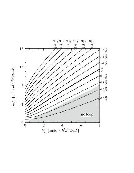
Figure 6: Contour plot of the maximum wave vector $k$ for energetic stability. Contours for $k\leq\pi/d$ corresponds to states on the lowest branch of the lowest band, and those for $k>\pi/d$ to states on the lower edge of the swallow tail at the zone boundary.

Figure 6 is a contour plot of the maximum wave vector for energetic stability as a function of $V_{0}$ and $nU_{0}$. Values of $k$ less than $\pi/d$ correspond to the lowest energy states for a given $k$, while higher values correspond to states on the lower edge of the swallow tail. As the plot shows, the range of $k$ values for which states are stable increases with increasing $nU_{0}$ and decreasing $V_{0}$. The numerical calculations in Fig. 6 are converged to within the thickness of the contour lines for $\nu_{\rm max}=3$ and $l_{\rm max}=3$.

A number of insights into the behavior of the contours may be obtained from analytical arguments. First, the intercepts on the $nU_{0}$ axis of the contours for the wave vector at which energetic stability sets in may be determined from the Landau criterion. For an interacting Bose gas with no lattice, energetic stability occurs when the velocity of the gas becomes equal to the sound speed $s$, Eq. (46). The velocity of the gas is $\hbar k/m$, and therefore the condition is

$$\frac{\hbar k}{m}=s\;\;{\rm or}\;\;\frac{nU_{0}}{E_{0}}=2\left(\frac{d}{\pi}\right)^{2}k^{2}.$$ (82)

The numerical results agree with this.

Figure 7: Contour plot of the maximum wave vector $k$ for dynamical stability (solid lines). The notation is the same as in Fig. 6. For comparison the corresponding results for energetic stability are shown by dotted lines.

A second general remark is that, for small $V_{0}$, one would expect on the basis of perturbation theory that the contours for energetic stability would behave as $V_{0}^{2}$, again in agreement with the numerical results. However, for high values of $nU_{0}$, the quadratic dependence holds only for a limited range of $V_{0}$. The contours are approximately linear at higher values of $V_{0}$, just as are those for the width of the swallow tail at the zone boundary (see Fig. 4). The wave vector of the tip of the swallow tail sets a natural limit to the wave vector at which instability sets in, and indeed this limit is approached for large $nU_{0}$.

A comparison of the width of the swallow tail (Fig. 4) and the stability boundary (Fig. 6) allow us to conclude that, within the range of parameters investigated, states on the lower edge of the swallow tail at the zone boundary are never stable for all $k$. For the conditions under which the spectrum is given by Fig. 1a, instability sets in around $k=1.7\pi/d$ and for the conditions appropriate for the spectrum shown in Fig. 1b, around $k=1.1\pi/d$.

IV.3.2 Dynamical stability

The boundary for dynamical stability is determined following a numerical procedure similar to the one above for energetic stability. On one side of the boundary, the operator $\hat{\sigma}_{z}\hat{B}$ has only real eigenvalues for all $q$, while on the other side it has some eigenvalues that are complex. The eigenvalues of $\hat{\sigma}_{z}\hat{B}$ are determined using the Mathematica^® routine “Eigenvalues”. With increasing $k$ (at fixed $nU_{0}$ and $V_{0}$), energetic instability first occurs for $q\rightarrow 0$, while dynamical instability first sets in at $q=\pi/d$. On the lowest branch of the lowest band, dynamical instability exists only for $k>\pi/2d$, in agreement with Fig. 1 of Ref. Wu and Niu (2001).

Figure 7 shows a contour plot of the maximum wave vector for dynamical stability as a function of $V_{0}$ and $nU_{0}$ as solid lines, and the corresponding contours for energetic stability are shown as dotted lines. The numerical calculations in Fig. 7 are converged to within the width of the contour lines for $\nu_{\rm max}=3$ and $l_{\rm max}=3$. For given $V_{0}$ and $nU_{0}$, the maximum wave vector for dynamical stability is always greater than that for energetic stability. The contours of the maximum wave vector for dynamical stability are nearly linear for the ranges of $V_{0}$ and $nU_{0}$ investigated. A comparison of the contours for energetic and dynamical stability in Fig. 7 shows that the stability boundaries almost coincide for larger values of $V_{0}$.

V Discussion and conclusions

Our analytical and numerical calculations show that the band structure of a Bose condensate in a one-dimensional optical lattice is affected dramatically by the presence of interactions between particles. The appearance of swallow-tail-like loop structures is a rather general phenomenon. They occur in the lowest band in the vicinity of the zone boundary, as reported earlier Diakonov et al. (2002), and also, as predicted in this paper, near the zone center in higher bands. Indeed, at band gaps at the zone boundary or at the zone center one expects such structures to appear quite generally on the band with lower energy if the effective interaction between particles is repulsive, the case studied in this paper. For an attractive effective interaction (negative scattering length), the loop structures would appear on the upper band at the gap. While macroscopic condensates with negative scattering length are unstable to collapse if the transverse extent of the cloud is large, it might be possible to investigate phenomena associated with swallow tails in such condensates if the condensate is tightly confined in the transverse directions.

Analytic results were derived using an approximate wave function containing either two plane waves (for states with wave vector close to the zone boundary) or three plane waves (for states with wave vectors close to zero). The coupling between plane wave components increases with the strengths of the interatomic interaction and of the potential $V_{0}$, and consequently, the approximate wave functions become less accurate. The potential induces couplings between plane waves whose wave vectors differ by only the smallest reciprocal lattice vectors $\pm 2\pi/d$, while the interaction term introduces couplings which are less restricted. The simple analytic expressions for the energy spectra are in good qualitative and, in some cases, quantitative agreement with the numerical results. At the zone boundary the approximate wave function coincides with the exact one, which accounts for the good agreement with the numerical results.

For swallow tails to appear, the interparticle interaction must exceed a critical value which depends on the band in question. We have derived a simple analytic expression, Eq. (20), for the width of the swallow tail around the zone boundary as a function of the interaction $nU_{0}$ and the potential $V_{0}$. According to the analytical models we have used, in the limit of a vanishing potential ($V_{0}\rightarrow 0$) the width of the swallow tail at the zone center behaves as $w=nU_{0}\pi/4E_{0}d$ and that at the zone boundary as $w=nU_{0}\pi/2E_{0}d$.

The physical interpretation of states on the upper edge of swallow tails is that they are periodic solitons. These states exist even in the absence of the lattice potential, and this accounts for the fact that the width of the swallow tails does not vanish when the lattice potential is absent.

With respect to experimental observability, an important question is whether or not the stationary states are stable. For conditions under which one does not expect swallow-tail structures in the lowest band, the stability of states has been explored previously by Wu and Niu Wu and Niu (2001), and for large interactions but only at the zone boundary in Ref. Wu et al. (2002). In the present work we have explored the stability of states on the swallow tail. States associated with the upper edge of the swallow tail are always energetically unstable, since they correspond to a saddle point in the energy landscape. The energetic and dynamical stability of the states corresponding to the lower edge of the swallow tail have been studied numerically, and we found that they become more stable as the strength of the interatomic interaction increases. We have not calculated growth times for unstable modes, but the calculations in Ref. Wu and Niu (2001) indicate that these are short compared with typical experimental times except under conditions very close to the threshold for instability. Thus we expect growth of instabilities to be an important effect in limiting the conditions under which states corresponding to the swallow tail may be investigated experimentally.

The general formalism for studying stability is rather cumbersome, but we showed in Sec. III.3 that for long-wavelength modes one may develop a hydrodynamic approach. The detailed numerical calculations indicate that energetic stability sets in at long wavelengths and therefore the properties of long-wavelength modes is of direct relevance for determining the limit of stability of a condensate. Using the hydrodynamic formalism, we derived a simple analytic expression for the stability limit of the states at the zone boundary, Eq. (79).

We have restricted our present study to stationary states in which the particle density is periodic with a period equal to the spacing $d$ of the lattice. However, as will be discussed elsewhere, stationary states with longer period, e.g. $2d$ or $3d$, exist. An example of a state with a particle density which has a period of two lattice spacings is a periodic soliton state, with one dark soliton for every two lattice cells. The difference in phase between two points separated by two lattice spacings, $\phi(x+2d)-\phi(x)=\pm\pi$, and therefore the wave vector is $\pm\pi/2d$.

In order to observe states corresponding to the lower edge of the swallow tail, it is desirable that the states be stable. To achieve this would require the mean-field energy $nU_{0}$ to be about an order of magnitude larger than in current experiments. The criterion for energetic stability at $k=\pi/d$ is $nU_{0}>2E_{0}$, corresponding to a a chemical potential $\mu=2E_{0}$ in the lowest band at the zone center, while in the experiment of Cataliotti et al. Cataliotti et al. (2001) the chemical potential was $\mu\approx 0.2E_{0}$.

Throughout our calculations we have assumed that the system is homogeneous in the directions transverse to the optical lattice. However, in actual experiments there is usually a confining potential in these directions. With sufficiently tight confinement in the transverse directions, a condensate is expected to behave quasi-one-dimensionally, as described in Refs. Jackson et al. (1998); Massignan and Modugno . Such condensates could provide suitable systems for observing some of the non-linear effects predicted in this paper.