Superconductivity of SrTiO_3-δ

Abstract

Superconducting SrTiO_3-δ was obtained by annealing single crystalline SrTiO₃ samples in ultra high vacuum. An analysis of the $V(I)$ characteristics revealed very small critical currents $I_{\mathrm{c}}$ which can be traced back to an unavoidable doping inhomogeneity. $R(T)$ curves were measured for a range of magnetic fields $B$ at $I\ll I_{\mathrm{c}}$, thereby probing only the sample regions with the highest doping level. The resulting curves $B_{\mathrm{c2}}(T)$ show upward curvature, both at small and strong doping. These results are discussed in the context of bipolaronic and conventional superconductivity with Fermi surface anisotropy. We conclude that the special superconducting properties of SrTiO_3-δ can be related to its Fermi surface and compare this finding with properties of the recently discovered superconductor MgB₂.

1 Introduction

It is well known that doped SrTiO₃ becomes superconducting with a transition temperature $T_{c}$ which strongly depends on the doping level Sch65 . Early theories of superconductivity in materials with small charge carrier densities considered a many-valley semiconductor band structure as beneficial for superconductivity due to an increased electron-phonon scattering rate Par69 . Indeed, first band structure calculations Kah64 predicted a Fermi surface of six disjoint ellipsoids for doped SrTiO₃. However, later calculations Mat72 , which are in good agreement with experimental results Gre79 , exhibited a Fermi surface of two sheets at the zone center. Despite of the low charge carrier density of doped SrTiO₃ and assuming no extraordinary electron-phonon scattering rate the appearance of superconductivity can be explained by a two-phonon mechanism Nga74 . Alternatively, a recent theoretical treatment predicts strong electron-phonon coupling due to reduced electronic screening at low doping Jar00 .
Due to the specific band structure and reduced interband scattering, so called two band superconductivity is possible in SrTiO₃. This expression describes the formation of distinct superconducting order parameters on the two sheets of the Fermi surface. Evidence for two band superconductivity in Nb-doped SrTiO₃, but not in SrTiO_3-δ, was found by tunneling spectroscopy performed with an STM Bin80 . Recently two band superconductivity attracted considerable interest because it was proposed to be realized in the new superconductor MgB₂ Gui01 .
Independently of the band structure considerations given above, doped SrTiO₃ is regarded as a candidate material for bipolaronic superconductivity Mic90 . The basic idea is that two polarons form a local pair called bipolaron. These bipolarons are charged bosons which can condense into a superfluid-like state. The possibility of bipolaronic superconductivity was extensively discussed for high temperature superconductors, but presumably cannot be applied to these materials Cha98 . However, in doped SrTiO₃ due to its huge dielectric polarizability ($\epsilon\simeq 300$) and low carrier density ($\simeq 10^{20}$cm^-1) Sch65 the possibility of polaron formation is obvious and experimental evidence for their formation exists Ger93 ; Eag96 ; Ang00 . However, pairing of polarons and the formation of itinerant bipolarons was not observed in any compound up to now.
In this paper we first describe the preparation of superconducting SrTiO_3-δ. It is shown that the doping of our samples is inhomogeneous. However, from $V(I)$ curves we determine a current which is small enough to probe only the superconducting surface region. Thus it is possible to measure the temperature dependence of the upper critical field of SrTiO_3-δ. $B_{c2}(T)$ curves of different samples are compared with the theories of bipolaron superconductivity and conventional superconductivity including Fermi surface anisotropy.

2 Preparation

The starting point of our preparation of SrTiO_3-δ samples were commercially available single crystalline SrTiO₃ (111) substrates of size $10\times 10\times 1$mm. The special substrate orientation was chosen because the generation of oxygen vacancies by annealing of (111) oriented SrTiO₃ proved to be more effective than that of (001) oriented samples. To obtain a geometry suitable for resistance measurements the substrates were polished down to a thickness of $\simeq 300{\rm\mu m}$ and cut into bars of width $\simeq 700{\rm\mu m}$. Two small Mo contact pads were deposited in a MBE chamber on each end of the SrTiO₃ stripes to allow 4-probe measurements of the sample resistance (see inset of Fig. 1).

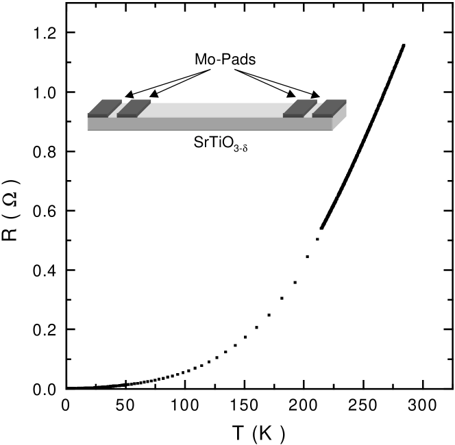
Figure 1: Temperature dependence of the resistance of metallic SrTiO_3-δ. Inset: Schematics of a SrTiO_3-δ sample with contact pads (not to scale).

The process of oxygen reduction was performed in a MBE chamber ($p\simeq 10^{-8}$mbar) at temperatures $T\simeq 1150$K for 1h.
Varying the annealing temperature by the amount of $\Delta T\simeq 50$K it was possible to tune the properties of the samples continuously from semiconducting to metallic Jou02 . A typical temperature dependence of the resistance of a metallic sample is shown in Fig. 1. All samples which showed metallic properties down to lowest temperatures became superconducting and $T_{c}$ decreased with decreasing annealing temperature. Employing the results of ref. Sch65 from the obtained $T_{c}$ values the charge carrier density of our samples can by estimated to be between $10^{18}$cm^-3 and $10^{19}$cm^-3. This is equivalent to a number of oxygen deficiencies per site of $\delta\simeq$$10^{-5}$ - $10^{-4}$. Because of this very small number of vacancies their clustering is not likely to appear and a rigid band shift of the Fermi level into the conduction band is expected Sha98 . The highest critical temperature obtained was $T_{c}=230$ mK. The excellent purity of our samples is reflected by residual resistance ratios of up to $RRR=R_{300K}/R_{0.3K}=3000$. If a homogeneous current distribution in the sample is assumed, specific residual resistances of $\rho(0.3{\rm K})\simeq 1\times 10^{-4}{\rm\Omega cm}$ are obtained.
However, recently it was pointed out that the doping level of reduced SrTiO_3-δ is inhomogeneous Szo02 . Reducing the thickness of an annealed sample by mechanical polishing could show that its specific room temperature resistance was macroscopically constant over its volume. Nevertheless, we observed that superconductivity is limited to a surface layer. When $\simeq 50{\rm\mu m}$ of SrTiO_3-δ were removed from the backside (side closest to the heating element) of an annealed sample a strong reduction of $T_{c}$ was obtained. Removing an additional $\simeq 50{\rm\mu m}$ layer from the front side destroyed superconductivity completely. However, removing only $\simeq 0.3{\rm\mu m}$ from both sides of an annealed sample by ion beam etching does not change its superconducting critical temperature. Thus we conclude that the oxygen content of our SrTiO_3-δ bars does not vary as strongly as in the samples of ref. Szo02 . Still, the doping level close to the surface is increased compared to the bulk volume.

3 V(I)-curves

For further investigation of the homogeneity of the superconducting state an increasing current was sent through the samples and the resulting voltage was measured. The obtained V(I)-curves are shown in Fig. 2. If a homogeneous current distribution in the SrTiO_3-δ bars is assumed, the calculated critical current densities will become very small and will be only of the order of $j_{c}\simeq 100{\rm A/cm^{2}}$.

Figure 2: $V(I)$-curves of superconducting SrTiO_3-δ in different applied magnetic fields $B$.

However, from the measured $V(I)$-curves it can be concluded that our samples consist of parallel normal conducting regions and superconducting regions. Thus the superconducting path for $T<T_{c}$ always remains in the critical regime and a current density and magnetic field dependent part of the total current flows in the normal conducting path. Qualitatively the measured $V(I)$-curves can be reproduced by a simple model: The sample is described by a parallel ohmic resistance $R_{N}$ and a type-II superconductor with a $V(I)$-characteristics governed by flux line dynamics. One of the simplest models for the description of these dynamics given by Anderson and Kim And64 is based on thermally activated motion of pinned flux lines. According to this description the electric field $E$ in the superconductor is given by equation 1 with the current density $j$, critical current density $j_{c}$, pinning potential $U_{P}$, specific normal resistance $\rho_{c}$ and temperature T.

$$E(j)=2\rho_{c}j_{c}e^{-U_{P}/k_{B}T}\sinh{\frac{jU_{P}}{j_{c}k_{B}T}}\,.$$ (1)

Fig. 3 shows calculated $V_{tot}(I_{tot})$-curves of a parallel normal conductor of resistance $R_{N}$ and a superconductor of the resistance given by equation 1.

Figure 3: Calculated $V(I)$-curves of a parallel circuit of a normal conductor and a superconductor with different critical current densities $j_{c}$ .

The qualitative agreement with the measured curves of Fig. 2 is obvious. Since neither the specific resistances of the normal and superconducting path nor the pinning potential of the flux lines is known, quantitative fits of the data cannot be performed.
However, the observed doping inhomogeneity has important implications for the measurement of the upper critical field as will be shown in the next section.

4 Upper critical field $\bf B_{c2}(T)$

From measurements of the upper critical field $B_{c2}(T)$ conclusions concerning Fermi surface and order parameter symmetry or even the mechanism of superconductivity are possible. Considering the inhomogeneities of the doping level of SrTiO_3-δ these measurements have to be performed carefully. From the analysis given above it is known that the samples consist of parallel normal conducting and superconducting regions with a distribution of critical temperatures $T_{c}$. Thus when $T_{c}(B)$ is determined by measuring resistance curves $R(T)$ or $R(B)$ it is important that the probe current does not produce local critical current effects. Provided a small enough current, the resistance of the current path with the highest doping level, i.e. in our range of doping highest superconducting $T_{c}$, dominates the result.
$B_{c2}(T)$ curves were determined by measuring the temperature dependence of the sample resistivity $R(T)$ in various magnetic fields. The probe current was chosen to be always more than an order of magnitude below the critical current $I_{c}$ as estimated from the strong increase in the $V(I)$-curve shown in the inset of Fig. 2. Additionally it was checked that temperature and width of the superconducting transition did not change when the probe current was doubled. The measured $R(T)$ curves of samples with low doping level show a small residual resistance in the superconducting state. This observation has to be related to the inhomogeneous doping (see above) and the fact that the contact wires were bonded to the upper sample surface. With a low doping level only the lower sample surface is superconducting and the resistance of the bulk material between the contact pads and lower sample surface persists in the superconducting state.
Samples with low $T_{c}$ in zero field ($T_{c}\simeq 100$ mK) showed broad superconducting transitions (Fig. 4).

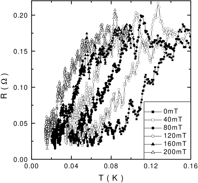
Figure 4: $R(T)$-curves of superconducting SrTiO_3-δ with low doping level in various applied magnetic fields $B$. Current perpendicular to magnetic field, magnetic field parallel (111).

The width of these transition slightly shrinks from $\Delta T\simeq 45$ mK to $\Delta T\simeq 35$ mK when the magnetic field is increased. $B_{c2}(T)$ can be determined either by choosing a midpoint, onset or downset criterion of the $R(T)$ curves. However, the choice of this criterion does only shift the upper critical field curve on the temperature axis but does not alter the qualitative features of its temperature dependence. In Fig. 5 $B_{c2}(T)$ curves are shown, which are determined by an onset (90%), midpoint (50%), and downset (10%) criterion. (B perpendicular (111): Only midpoint criterion shown for clarity). This SrTiO_3-δ sample has a low doping level and the magnetic field orientation was parallel or perpendicular to the sample surface, i.e. perpendicular or parallel to the crystallographic (111)-direction.

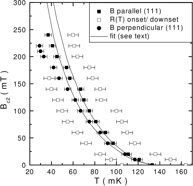
Figure 5: $B_{c2}(T)$-curves of superconducting SrTiO_3-δ with low doping level. Current direction perpendicular to the magnetic field. Field orientation parallel to sample surface, i.e. perpendicular (111), or perpendicular to sample surface, i.e. parallel (111). The fits shown are according to a theory Ale87 of bipolaronic superconductivity (see text).

The observed directional anisotropy may either reflect crystallographic anisotropy (cubic to tetragonal phase transition at $T=110K$ Mat72 ) or the depth profile of the doping level. However, the fact that the critical field oriented perpendicular to the polished sample surface is larger than oriented parallel to the sample proves that nucleation of superconductivity at the sample surface ($B_{c3}$) has no influence and that actually $B_{c2}$ is measured.
The most striking feature of the $B_{c2}(T)$ curves of samples with low doping level is their pronounced positive curvature. Such a positive curvature of the temperature dependence of the upper critical field is predicted by a theory of bipolaronic superconductivity. According to Alexandrov et al. Ale87 $B_{c2}(T)$ should be given by equation 2

$$B_{c2}(T)\propto\frac{1}{T}\left(1-\left(\frac{T}{T_{c}}\right)^{3/2}\right)^{3/2}\,.$$ (2)

The divergence at $T=0$K in this equation results from an approximation in ref. Ale87 . Fits according to equation 2 are plotted in Fig. 5. Reasonable agreement with the measured data is observed for magnetic fields $B<150$mT. For increased magnetic fields the fit deviates from the measured data which could be explained by the approximations of theory mentioned above. However, alternative explanations for the observed positive curvature in $B_{c2}(T)$ are possible as will be shown below.
More reliable $B_{c2}(T)$ data could be obtained for SrTiO_3-δ samples with increased doping level due to a strongly reduced and magnetic field independent superconducting transition width of $\Delta T\simeq 3$ mK. Measured $R(T)$ curves in various magnetic fields of a sample with high doping level are shown in Fig. 6.

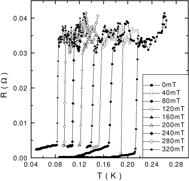
Figure 6: $R(T)$-curves of superconducting SrTiO_3-δ with high doping level in various applied magnetic fields $B$. Current perpendicular to magnetic field, magnetic field parallel (111).

The foot of the resistive transition has to be related to the inhomogeneous doping as well. Obviously, the backside of the sample has an increased doping level, whereas the front side with the contact pads shows a reduced $T_{c}$ with broad transition (lower doping level). Based on the $R(T)$ data the temperature dependence of the upper critical field is determined by the midpoints of the sharp superconducting transitions (Fig. 7).

x

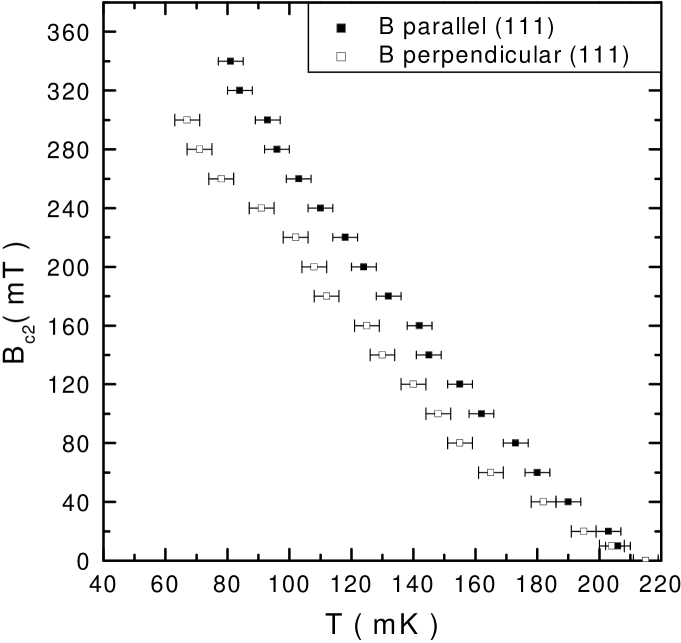
Figure 7: $B_{c2}(T)$-curves of superconducting SrTiO_3-δ with high doping level. Current direction perpendicular to the magnetic field. Field orientation parallel to sample surface, i.e. perpendicular (111), or perpendicular to sample surface, i.e. parallel (111).

Only a weak positive curvature of $B_{c2}(T)$ is obtained, much less pronounced than from samples of reduced doping level. Thus it is not possible to fit this data with the bipolaron theory (Eq. 2).
The conventional theory of the upper critical field in isotropic weak coupling superconductors by Helfand and Werthammer Hel66 predicts a negative curvature of $B_{c2}(T)$ for all temperatures. However, this also is in contradiction to the $B_{c2}(T)$ data obtained for SrTiO_3-δ. For an applicable theoretical description in the framework of conventional superconductivity the strongly anisotropic Fermi surface of SrTiO_3-δ has to be taken into account.
For simplicity we consider only orbital pair breaking and a single sheet anisotropic Fermi surface. A formulation for this case on the basis of the linearized Gor’kov gap equation has been put forward by Youngner and Klemm You80 . In the clean limit, it reduces to the self-consistency equation

$$\ln t=\sum_{\nu=-\infty}^{\infty}\left[\frac{1}{|2\nu+1|}\left(-1+\int d\hat{\rho}N(\hat{\rho})f(z_{\nu,\hat{\rho}})\right)\right]\,,$$ (3)

where $t=T_{\mathrm{c}}/T_{\mathrm{c0}}$ is the dimensionless critical temperature,

$$f(z_{\nu,\hat{\rho}})=\sqrt{\pi}z_{\nu,\hat{\rho}}\exp(z_{\nu,\hat{\rho}}^{2})\,{\rm erfc}(z_{\nu,\hat{\rho}})\,,$$ (4)

and

$$z_{\nu,\hat{\rho}}=\frac{t\,|2\nu+1|}{\sqrt{2h}}\frac{v_{{\rm F}}}{|v_{\perp}(\hat{\rho})|}\,.$$ (5)

Here, the dimensionless magnetic field

$$h=H_{{\rm c2}}\,e\hbar v_{{\rm F}}^{2}/(2\pi k_{{\rm B}}T_{{\rm c0}})^{2}$$ (6)

is defined in terms of some average Fermi velocity $v_{{\rm F}}$ and the zero-field critical temperature; its absolute scale will be unimportant for the final results. Furthermore, $v_{\perp}(\hat{\rho})$ denotes the component of the Fermi velocity in direction $\hat{\rho}$ which is perpendicular to the magnetic field. A simple model for an anisotropic Fermi surface with tetragonal symmetry (with the magnetic field in $(001)$ direction) is given in polar coordinates by

$$|v_{\perp}(\hat{\rho})|=v_{F}\sin(\Theta)[1+b\cos(4\phi)]\,,\quad$$ (7)

$$N(\hat{\rho})\propto\frac{1}{1+b\cos(4\phi)}\,,$$ (8)

where $0\leq b<1$ is the anisotropy parameter and the density of states is normalized to unity: $\int d\hat{\rho}N(\hat{\rho})=1$. We solve Eq. 3 for $h$ at fixed $t$ in a bracketing secant scheme until the error in $t$ (i.e., the difference between the exponentiated right hand side of Eq. 3 and $t$) is smaller than $10^{-4}$. Within this scheme, we use the cutoff $|\nu|\leq 300$; the irreducible part of the Fermi surface ($0\leq\cos\Theta\leq 1$, $0\leq\phi\leq\pi/4$) is sampled by $10^{3}$ patches. The maximum relative error in $h$ introduced by cutoff and discretization is estimated as $10^{-3}$. In order to avoid numerical instabilities, we use in equation 4 the asymptotic expansion $f(z)\approx 1-\frac{1}{2}z^{-2}+\frac{3}{4}z^{-4}$ for $z>20$. A comparison between theory and experiment is shown in Fig. 8.

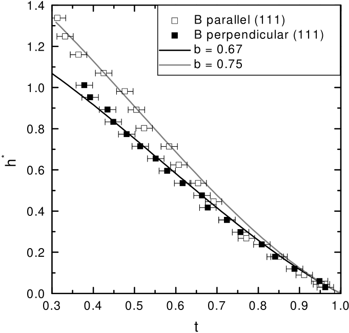
Figure 8: Comparison between the normalized temperature dependence of the upper critical field $h^{*}(t)$ and fits based on the linearized Gor’kov gap equation with different anisotropy parameter $b$.

Here, the experimental data has been converted to a dimensionless temperature using $T_{{\rm c0}}=214$ mK. Furthermore, all magnetic fields have been rescaled so that the derivative $dh^{*}/dt|_{t=1}=-1$ for each curve; note that this rescaling procedure is somewhat ambiguous for the experimental data. Excellent agreement is observed between the data measured parallel to $(111)$ and the theory for a value $b=0.67$ of the anisotropy parameter. This value implies a ratio of 5 of the maximum to the minimum Fermi velocity which is well within the limits discussed in the literature Mat72 . The fact that the theory for magnetic field in $(001)$ direction agrees so well with the experimental observation for field in $(111)$ direction supports our assumption that the overall variation of the Fermi velocity (and of the density of states) is more important than the precise shape of its distribution. Less satisfactory agreement is seen when the magnetic field is in-plane, i.e., perpendicular to the $(111)$ direction. Here, a stronger anisotropy $b=0.75$ is required for matching the region $t<0.6$; larger discrepancies remain near $t\simeq 0.75$. An application of this theory to the $B_{c2}(T)$ data of SrTiO_3-δ samples with low doping level fails to reproduce the measured strong curvature in the same temperature range.
In principle the qualitative difference of the $B_{c2}(T)$ data of samples with low and high doping could be associated with a crossover of the mechanism of superconductivity. For bipolaronic superconductivity above some critical doping it is generally expected that superconductivity is destroyed Ale94 . However, the doping level of our samples is well below the doping level with maximum $T_{c}$ Sch65 . Thus if bipolaronic superconductivity is realized in doped SrTiO₃, we would expect it to be realized in all of our samples. Assuming a doping independent mechanism of superconductivity in SrTiO_3-δ, the bipolaron theory can not be applied at all.
One explanation for the discrepancies between samples with low and high doping is inhomogeneous doping of the samples with low charge carrier density resulting in domains with different $T_{c}$, which influence the curvature of $B_{c2}(T)$. However, the samples with increased charge carrier density show sharp superconducting transitions, i.e. a homogeneously doped sample region is probed. The $B_{c2}(T)$ curves of these samples could be fitted by a conventional theory including Fermi-surface anisotropy. Thus it appears likely that the mechanism of superconductivity of SrTiO_3-δ is conventional independent of the doping level.
The observed positive curvature of $B_{c2}(T)$ is not unique to SrTiO_3-δ. An alternative approach results in very similar curves and considers an effective two-band model, i.e. two groups of electrons with different superconducting energy gaps Shu98 (applied for borocarbides). Similar behavior was observed in the recently discovered superconductor MgB₂ Lim01 ; Sol02 . There is strong evidence for the contribution of two different areas of the Fermi surface to the superconducting state of this compound Iav02 ; Bou02 . Very recently, $B_{c2}(T)$ curves of MgB₂ with positive curvature were calculated considering superconducting gaps on two Fermi sheets as a particular case of gap anisotropy Mir03 .

5 Conclusions

Considering the properties of self doped, i.e. ultra high vacuum annealed, SrTiO_3-δ it is necessary to take an inhomogeneous doping profile into account. Nevertheless, by careful adjustment of the probe current the upper critical field of high purity samples could be investigated. Samples with low doping level show a strong positive curvature of the $B_{c2}(T)$-curve, which is still present, but less pronounced for samples with increased doping level. The theory of bipolaronic superconductivity predicts a positive curvature of $B_{c2}(T)$ and can be used for a fit of reasonable agreement with the $B_{c2}(T)$-curves of samples with low doping level. However, more reliable data obtained from samples with increased doping level can not be fitted by the bipolaron theory, which discards its applicability. A conventional explanation for the observed temperature dependence of the upper critical field can be given by considering the strongly anisotropic Fermi surface of SrTiO_3-δ. Good fits of $B_{c2}(T)$ were obtained using a concept which goes beyond the Helfand-Werthamer theory by taking this Fermi surface anisotropy into account. Thus the unusual superconducting properties of SrTiO_3-δ can be explained in the framework of a conventional pairing mechanism.

References

- (1) J. F. Schooley, W. R. Hosler, E. Ambler, J. H. Becker, M. L. Cohen, and C. S. Koonce, Phys. Rev. Lett. 14, 305 (1965).
- (2) M. L. Cohen in Superconductivity, edited by R. D. Parks (Marcel Dekker, New York 1969), chap.12.
- (3) A. H. Kahn and A. J. Leyendecker, Phys. Rev. 135, A1321 (1964).
- (4) L. F. Mattheiss, Phys. Rev. B, 6, 4740 (1972).
- (5) B. Gregory, J. Arthur, and G. Seidel, Phys. Rev. B 19, 1039 (1979).
- (6) K. L. Ngai, Phys. Rev. Lett. 32, 215 (1974).
- (7) T. Jarlborg, Phys. Rev. B 61, 9887 (2000).
- (8) G. Binnig, A. Baratoff, H. E. Hoenig, and J. G. Bednorz, Phys. Rev. Lett. 45, 1352 (1980).
- (9) F. Giubileo, D. Roditchev, W. Sacks, R. Lamy, D. X. Thanh, J. Klein, S. Miraglia, D. Fruchart, J. Marcus, and Ph. Monod, Phys. Rev. Lett. 87, 177008 (2001).
- (10) R. Micnas, J. Ranninger, and S. Robaszkiewicz, Rev. Mod. Phys. 62, 113 (1990).
- (11) B. K. Chakraverty, J. Ranninger, and D. Feinberg, Phys. Rev. Lett. 81, 433 (1998).
- (12) F. Gervais, J. L. Servoin, A. Baratoff, J. G. Bednorz, and G. Binnig, Phys. Rev. B 47, 8187 (1993).
- (13) D. M. Eagles, M. Georgiev, P. C. Petrova, Phys. Rev. B 54, 22 1996).
- (14) ChenAng, ZhiYu, ZhiJing, P. Lunkenheimer, and A. Loidl, Phys. Rev. B 61, 3922 (2000).
- (15) M. Jourdan and H. Adrian, Physica C, 388-389, 509 (2003).
- (16) N. Shanti and D. D. Sarma, Phys. Rev. B 57, 2153 (1998).
- (17) K. Szot, W. Speier, R. Carius, U. Zastrow, and W. Beyer, Phys. Rev. Lett. 88, 075508 (2002).
- (18) P. W. Anderson and Y. B. Kim, Rev. Mod. Phys. 36, 39 (1964).
- (19) A. S. Alexandrov, D. A. Samarchenko, and S. V. Traven, Sov. Phys. JETP 66, 567 (1987).
- (20) E. Helfand and N. R. Werthamer, Phys. Rev. Lett. 13, 686 (1964); Phys. Rev. 147, 288 (1966).
- (21) D. W. Youngner and R. A. Klemm, Phys. Rev. B 21, 3890 (1980).
- (22) A. S. Alexandrov and N. F. Mott, Rep. Prog. Phys. 57 1197 (1994).
- (23) S. V. Shulga, S. -L. Drechsler, G. Fuchs, and K. -H. Müller, K. Winzer, M. Heinecke, and K. Krug, Phys. Rev. Lett. 80, 1730, (1998).
- (24) O. F. de Lima, R. A. Ribeiro, M. A. Avila, C. A. Cardoso, and A. A. Coelho, Phys. Rev. Lett. 86, 5974 (2001).
- (25) A. V. Sologubenko, J. Jun, S. M. Kazakov, J. Karpinski, and H. R. Ott, Phys. Rev. B 65 180505 (2002).
- (26) M. Iavarone, G. Karapetrov, A. E. Kwok, G. W. Crabtree, and D. G. Hinks, W. N. Kang, Eun-Mi Choi, Hyun Jung Kim, Hyeong-Jin Kim, and S. I. Lee, Phys. Rev. Lett. 89, 187002 (2002).
- (27) F. Bouquet, Y. Wang, I. Sheikin, T. Plackowski, and A. Junod, S. Lee and S. Tajima, Phys. Rev. Lett. 89, 257001 (2002).
- (28) P. Miranovic, K. Machida and V. G. Kogan, J. Phys. Soc. Jpn. 72, 221 (2003).