Mode-coupling approach to non-Newtonian Hele-Shaw flow

Abstract

The Saffman-Taylor viscous fingering problem is investigated for the displacement of a non-Newtonian fluid by a Newtonian one in a radial Hele-Shaw cell. We execute a mode-coupling approach to the problem and examine the morphology of the fluid-fluid interface in the weak shear limit. A differential equation describing the early nonlinear evolution of the interface modes is derived in detail. Owing to vorticity arising from our modified Darcy’s law, we introduce a vector potential for the velocity in contrast to the conventional scalar potential. Our analytical results address how mode-coupling dynamics relates to tip-splitting and side branching in both shear thinning and shear thickening cases. The development of non-Newtonian interfacial patterns in rectangular Hele-Shaw cells is also analyzed.

I Introduction

The celebrated Saffman-Taylor instability MW_3 arises when a less viscous fluid pushes a more viscous one in the thin gap of a Hele-Shaw cell. The less viscous fluid can be either injected at an end of a channel-shaped cell (rectangular geometry) MW_3 , or from the center of the cell (radial geometry) Pat . In both geometries the interface separating the fluids may deform, leading to the formation of fingerlike patterns, commonly known as viscous fingers. During the last four decades, the viscous fingering instability has been extensively studied, both theoretically MW_1 and experimentally MW_1b . Much of the research in this area has examined the case in which the fluids involved are Newtonian. For Newtonian fluids, it is observed that the fingers grow and compete dynamically, resulting in a single stable finger in the rectangular geometry, and in patterned structures markedly characterized by the spreading, and subsequent splitting of the finger tips in the radial setup.

A whole different class of interfacial patterns arise when the Saffman-Taylor instability is studied by taking the displaced fluid as non-Newtonian MW_1b ; Van . In contrast to most Newtonian fluids, non-Newtonian fluids differ widely in their hydrodynamic properties, with different fluids exhibiting a range of effects from elasticity and plasticity to shear thinning and shear thickening. Experiments using non-Newtonian fluids in radial and rectangular Hele-Shaw cells have revealed a wide variety of new patterns, showing snowflake-like shapes MW_1b ; Buka and fracturelike structures Lemaire ; Zhao . Instead of the traditional, tip-splitting-dominated Newtonian patterns, these experiments MW_1b ; Buka ; Lemaire ; Zhao exhibit dendritic fingers and side branching. This morphological diversity and rich dynamical behavior motivated a number of theoretical studies of the problem Sader ; Bonn ; Kondic_96 ; Kondic_98 ; Kondic_long . One major difficulty faced by researchers is that, as opposed to the Newtonian case, the pressure field is no longer Laplacian. This implies a serious theoretical challenge, since a priori one would not be allowed to directly apply a Darcy’s law approach to attack the problem.

The instability of radial Hele-Shaw flows involving non-Newtonian fluids has been studied theoretically by Sader et al. Sader . They considered power law fluids, and performed a linear stability analysis without making use of Darcy’s law. Essentially, they showed that decreasing the power law index dramatically increases the growth rates leading to a more rapid development of the fingering patterns. A Darcy’s law-type approach has been proposed by Bonn and collaborators Bonn . Bonn et al. suggested a modified Darcy’s law including a shear rate dependent viscosity, and showed that, within their approach, the pressure field remains Laplacian. In a series of interesting papers Kondic et al. Kondic_96 ; Kondic_98 , and subsequently Fast et al. Kondic_long extended reference Bonn ideas and derived a generalized Darcy’s law from first principles, where viscosity depends upon the squared pressure gradient. It turns out that the Darcy’s law formula proposed by Bonn et al. Bonn follows from the more basic version rigorously derived by Kondic et al. Kondic_96 ; Kondic_98 . Efficient numerical simulations performed in references Kondic_98 ; Kondic_long have shown that shear thinning can suppress tip-splitting and leads to the formation of dendritic structures, presenting a clear side branching behavior.

Theoretical studies of the fully nonlinear stages of Hele-Shaw flow with non-Newtonian fluids rely heavily on intensive numerical simulations Kondic_98 ; Kondic_long . On the analytical side, the structure of the fingering dynamics in such complex fluids is largely restricted to linear stability investigations Sader ; Kondic_96 . Much less attention has been paid to the analytical investigation of the dynamics that bridges the initial (purely linear) and final (fully nonlinear) time regimes. In addition, theoretical as well as experimental analyses of flow of shear thickening fluids in Hele-Shaw cells still need to be addressed. In this paper we carry out the analytical weakly nonlinear analysis for the intermediate stages of evolution, and examine both shear-thinning and shear thickening cases. We adapt a weakly nonlinear approach originally developed to study Newtonian Hele-Shaw flows MW_rectang ; MW_rad , to the non-Newtonian situation. We focus on the onset of the nonlinear effects, and try to understand how mode-coupling dynamics leads to basic morphological features and behaviors observed in non-Newtonian Hele-Shaw flows.

The article is organized as follows: section II formulates our theoretical approach. We perform a Fourier decomposition of the interface shape, and from an alternative form of Darcy’s law study the influence of weak shear effects on the development of interfacial patterns. In contrast to the analysis for Newtonian fluids, conventionally based on a scalar velocity potential, we employ a vector velocity potential capable of describing vorticity arising from the non-Newtonian fluid flow. Coupled, nonlinear, ordinary differential equations governing the time evolution of Fourier amplitudes are derived in detail. Section III discusses both linear and weakly nonlinear dynamics. It concentrates on the effect of shear thinning and shear thickening on finger tip-splitting and side branching. Section III.1 briefly discusses our linear stability results. Linear results are useful and instructive, but do not allow accurate predictions of important interfacial features. In section III.2 we show that some of such features can indeed be predicted and more quantitatively explained by our analytical mode-coupling approach. At second order we find a mechanism for finger tip-splitting in non-Newtonian Hele-Shaw flow: it is suppressed (favored) for shear thinning (thickening) fluids. Our results indicate absence of side branching in the weak shear limit and early flow stages, but suggest that it could be enhanced (inhibited) for shear thinning (thickening) fluids. Section III.3 discusses mode-coupling in rectangular flow geometry. Our chief conclusions are summarized in Sec. IV.

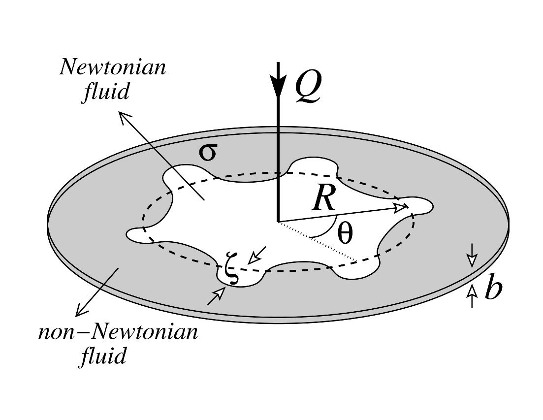
Figure 1: Schematic configuration of radial flow in a Hele-Shaw cell. The inner fluid is Newtonian and has negligible viscosity. The outer fluid is non-Newtonian. All physical parameters are defined in the text.

II The mode-coupling differential equation

The Hele-Shaw cell (Fig.1) consists of two parallel plates separated by a small distance. The cell thickness $b$ is considered to be much smaller that any other length scale in the problem, so that the system is essentially two-dimensional. Consider the displacement of a viscous, non-Newtonian fluid by a Newtonian fluid of negligible viscosity in such confined geometry. The surface tension between the fluids is denoted by $\sigma$. The Newtonian fluid is injected at a constant areal flow rate $Q$ at the center of the cell.

The initial circular fluid-fluid interface is slightly perturbed, ${\cal R}=R(t)+\zeta\left(\theta,t\right)$ ($\zeta/R\ll 1$), where the time dependent unperturbed radius is given by

$$R(t)=\sqrt{R_{0}^{2}+\frac{Qt}{\pi}},$$ (1)

$R_{0}$ being the unperturbed radius at $t=0$. The interface perturbation is written in the form of a Fourier expansion

$$\zeta(\theta,t)=\sum_{n=-\infty}^{+\infty}\zeta_{n}(t)\exp{\left(in\theta\right)},$$ (2)

where $\zeta_{n}(t)=(1/2\pi)\int_{0}^{2\pi}\zeta(\theta,t)\exp{(-in\theta)}~{}{\rm d}\theta$ denotes the complex Fourier mode amplitudes and $n$=0, $\pm 1$, $\pm 2$, $...$ is the discrete polar wave number. In our Fourier expansion (2) we include the $n=0$ mode to keep the area of the perturbed shape independent of the perturbation $\zeta$. Mass conservation imposes that the zeroth mode is written in terms of the other modes as $\zeta_{0}=-(1/2R)\sum\limits_{n\neq 0}|\zeta_{n}(t)|^{2}$.

The relevant hydrodynamic equation for Newtonian Hele-Shaw flows, Darcy’s law MW_3 ; MW_1 , states that the gradient of the pressure is proportional to the fluid velocity, and oriented in the opposite direction with respect to the fluid flow

$${\nabla}p=-\frac{12\mu}{b^{2}}~{}{\bf v},$$ (3)

where ${\bf v}={\bf v}(r,\theta)$ and $p=p(r,\theta)$ are, respectively, the gap-averaged velocity and pressure in the fluid. The viscosity of the fluid is represented by $\mu$. To model non-Newtonian Hele-Shaw flows, we use a suitable form of the Darcy’s law in the weak shear thinning or thickening limit. We follow Bonn et al. Bonn and consider their shear rate dependent viscosity in the weak non-Newtonian limit $(\omega\tau)^{2}\ll 1$

$${\mu(\omega^{2})}\approx{\mu_{0}\left[1-\left(1-\alpha\right)\omega^{2}\tau^{2}\right]},$$ (4)

where $\omega\approx v/b$ is the shear rate, $v=|{\bf v}|$, $\tau$ denotes the characteristic relaxation time of the fluid, and $\mu_{0}$ is a constant, zero-shear viscosity. The parameter $\alpha$ measures the shear dependence: $\alpha=1$ corresponds to the Newtonian fluids, and $\alpha<1$ ($\alpha>1$) gives the shear thinning (thickening) case.

By substituing Eq. (4) into Eq. (3) we obtain an alternative form of Darcy’s law ideally suited to describe weak non-Newtonian effects

$${\nabla P}=-{\bf v}~{}+~{}\delta v^{2}{\bf v}.$$ (5)

Here $P=[b^{2}/(12\mu_{0})]~{}p$ represents a generalized pressure field, and $\delta=(1-\alpha)(\tau/b)^{2}$ is a small parameter that expresses the non-Newtonian nature of the displaced fluid: $\delta=0$ corresponds to the Newtonian case, while $\delta>0$ ($\delta<0$) describes the shear thinning (thickening) case. Taking the divergence of Eq. (5) and using incompressibility ($\nabla\cdot{\bf v}=0$) the pressure is seen to be anharmonic (nonvanishing Laplacian). Our subsequent analysis incorporates this effect, in contrast to the treatment in Ref. Bonn . Indeed, an alternate route to our Eq. (5) is to start with viscosity depending on the square of the pressure gradient (as in Kondic, et al. Kondic_96 ), then approximate the pressure gradient with the velocity for small $\delta$.

Our pertubative approach keeps terms up to the second order in $\zeta$ and up to first order in $\delta$. Considering the fact that the viscosity of the Newtonian fluid is negligible, the generalized pressure jump condition at the interface can be written as MW_1

$$P|_{{\cal R}}=-\gamma~{}\kappa_{\|}|_{{\cal R}},$$ (6)

where $\gamma=b^{2}\sigma/(12\mu_{0})$ and $\kappa_{\|}$ is the curvature in the direction parallel to the plates.

The weakly nonlinear approach to radial, Newtonian Hele-Shaw flow developed in reference MW_rad , related the fluid velocity to a scalar velocity potential ${\bf v}=-\nabla\phi$, this replacement made possible by the irrotational nature of the flow for Newtonian fluids. For non-Newtonian fluids, in contrast, flows governed by the modified Darcy’s law (5) exhibit vorticity. Hence we perform our calculations using a vector potential ${\bf v}=\nabla\times{\bf A}$. The most general form of the vector potential can be written as

$${\bf A}=\left[\frac{Q}{2\pi}\theta+\sum_{m,n\not=0}A_{mn}\left(\frac{R}{r}\right)^{m}\exp{(in\theta)}\right]\hat{\bf z},$$ (7)

where $A_{mn}$ are the Fourier coefficients of the velocity vector potential and $\hat{\bf z}$ is the outward unit-normal to the upper cell plate. The radial and polar components of the fluids velocities are

$${v_{r}}=\frac{Q}{2\pi r}+\sum_{m,n\not=0}inA_{mn}\left(\frac{R^{m}}{r^{m+1}}\right)\exp{(in\theta)},$$ (8)

and

$${v_{\theta}}=\sum_{m,n\not=0}mA_{mn}\left(\frac{R^{m}}{r^{m+1}}\right)\exp{(in\theta)}.$$ (9)

Note that the vector potential reduces to the unperturbed steady flow with a circular interface ($v_{r}=Q/2\pi r$, $v_{\theta}=0$) when $R\rightarrow 0$ and also when $r\rightarrow\infty$.

We exploit the fact that $\nabla P$ must be curl free, and impose the so-called solvability condition $\nabla\times\nabla P=0$. It simplifies the general form of the vector potential expansion given in Eq. (7). The solvability condition reveals that, without loss of generality, one can rewrite the vector potential as

$${\bf A}=\left\{\frac{Q}{2\pi}\theta+\sum_{n\not=0}A_{n}\left(\frac{R}{r}\right)^{|n|}\exp{\left(in\theta\right)}+\delta\left[\sum_{n\not=0}B_{n}\left(\frac{R}{r}\right)^{|n|}\frac{1}{r^{2}}\exp{(in\theta)}\right]\right\}~{}\hat{\bf z},$$ (10)

replacing the array of coefficients $A_{mn}$ with the simpler set of $A_{n}$ and $B_{n}$. Observe that the vector potential (10) is simply a superposition of a purely Newtonian term ($\propto\delta^{0}$, coefficients $A_{n}$) and a non-Newtonian contribution ($\propto\delta^{1}$, coefficients $B_{n}$)

$${\bf A}={\bf A}_{N}+{\bf A}_{NN}.$$ (11)

The flow described by ${\bf A}_{N}$ is irrotational, while ${\bf A}_{NN}$ has a curl.

Similarly, we express the pressure of the outer fluid as a sum of Newtonian and non-Newtonian pressures, and propose a general form for their Fourier expansion

$$P=P_{N}+P_{NN},$$ (12)

where

$$P_{N}=-\frac{Q}{2\pi}\log{\left(\frac{r}{R}\right)}+\sum_{n\not=0}p_{n}\left(\frac{R}{r}\right)^{|n|}\exp{(in\theta)},$$ (13)

and

$$P_{NN}=\delta\left[-\left(\frac{Q}{2\pi}\right)^{3}\frac{1}{2r^{2}}+\sum_{n\not=0}q_{n}\left(\frac{R}{r}\right)^{|n|}\frac{1}{r^{2}}\exp{(in\theta)}\right].$$ (14)

The gradient of the complex pressure field (12) must satisfy the non-Newtonian Darcy’s law given by Eq. (5). By inspecting the $r$ and $\theta$ components of (5), and by examining the Newtonian and non-Newtonian components of it, we can express the Fourier coefficients of $P_{N}$, $P_{NN}$ and ${\bf A}_{NN}$ in terms of the Fourier coefficients of ${\bf{A}}_{N}$,

$$p_{n}={\rm sgn}(n)\left(iA_{n}\right),$$ (15)

$$q_{n}=-iA_{n}\beta(n)\frac{n}{|n|}\left(\frac{Q}{2\pi}\right)^{2}+\frac{Q}{4\pi\left(|n|+1\right)}\sum_{m\not=0,m\not=n}mA_{m}\left(n-m\right)A_{n-m}~{}k\left(n,m\right),$$ (16)

$$B_{n}=-A_{n}\alpha(n)\left(\frac{Q}{2\pi}\right)^{2}+\frac{Q}{4\pi\left(|n|+1\right)}\sum_{m\not=0,m\not=n}m\left(iA_{m}\right)\left(n-m\right)A_{n-m}~{}h\left(n,m\right),$$ (17)

where in order to keep the results in a compact form, we introduced the coefficients

$${\alpha\left(n\right)}={\frac{|n|\left(|n|-1\right)}{2\left(|n|+1\right)}},$$ (18)

$${\beta\left(n\right)}={\frac{|n|\left(|n|+3\right)}{2\left(|n|+1\right)}},$$ (19)

$$h\left(n,m\right)=\left(|n|+2\right){\rm sgn}(n-m)-\frac{n}{2}\left\{3-{\rm sgn}\left[m\left(n-m\right)\right]\right\},$$ (20)

and

$$k\left(n,m\right)=-n\,{\rm sgn}(n-m)+\frac{1}{2}\left(|n|+2\right)\left\{3-{\rm sgn}\left[m\left(n-m\right)\right]\right\}.$$ (21)

Note that ${\rm sgn}(n)=1$ if $n>0$ and ${\rm sgn}(n)=-1$ if $n<0$.

Using Eqs. (15)-(17), which are consistent with the solvability condition and Darcy’s law (5), we can derive the general expression of the vector potential Fourier coefficients in terms of the perturbation amplitudes. To fulfill this goal, consider the kinematic boundary condition MW_1 ; MW_1b

$${\frac{\partial\cal R}{\partial t}}=\left[\frac{1}{r}\frac{\partial\cal R}{\partial\theta}\left(-v_{\theta}\right)+v_{r}\right]_{|_{\cal R}},$$ (22)

which states that the normal components of each fluid’s velocity at the interface equals the velocity of the interface itself. By expanding Eq. (22) up to the second order in $\zeta$ and up to first order in $\delta$ we find the coefficient of the vector potential corresponding to the $n$-th evolution mode, $A_{n}^{(k)}$, in terms of $\delta$ and the $k$-th order in $\zeta$ ($k$ = 1, 2)

$${iA_{n}^{\left(1\right)}(t)}=\left[\frac{R}{n}\dot{\zeta}_{n}+\frac{\dot{R}}{n}\zeta_{n}\right]\left[1+\delta{\dot{R}}^{2}\alpha\left(n\right)\right],\\$$

$${iA_{n}^{\left(2\right)}(t)} = \frac{{\dot{R}}}{R}\sum_{m\not=0,n}\left[\frac{|m|}{m}+\delta{\dot{R}}^{2}u(n,m)\right]\zeta_{m}\zeta_{n-m}+\sum_{m\neq 0,n}\left[\frac{1}{n}+\frac{|m|}{m}+\delta{\dot{R}}^{2}v(n,m)\right]\dot{\zeta}_{m}\zeta_{n-m}$$

$$- \frac{\delta{\dot{R}}R}{2\left(|n|+1\right)}\sum_{m\neq 0,n}h(n,m)~{}\dot{\zeta}_{m}\dot{\zeta}_{n-m}-\frac{\delta{\dot{R}}^{2}}{2\left(|n|+1\right)}\sum_{m\neq 0,n}h(n,m)~{}\zeta_{m}\dot{\zeta}_{n-m},$$

where the overdot denotes total time derivative, ${\dot{R}}=Q/(2\pi R)$ represents the unperturbed interface velocity, and the coefficients

$${u\left(n,m\right)}=\alpha(n)\frac{|m|}{m}-2\frac{\alpha(m)}{m}-\frac{h(n,m)}{2\left(|n|+1\right)},$$ (24)

$${v\left(n,m\right)}=\alpha(n)\left(\frac{1}{n}+\frac{|m|}{m}\right)-2\frac{\alpha(m)}{m}-\frac{h(n,m)}{2\left(|n|+1\right)}.$$ (25)

To conclude our derivation we need one more step. The vector potential coefficients can be introduced into the pressure jump condition (Eq.(6)) and using Darcy’s law (Eq.(5)) one can finally find the equation of motion for perturbation amplitudes $\zeta_{n}$. We present the evolution of the perturbation amplitudes in terms of $\delta$ and the $k$-th order in the perturbation amplitude $\zeta$

$${\dot{\zeta}_{n}}=\dot{\zeta}_{n}^{\left(1\right)}+\dot{\zeta}_{n}^{\left(2\right)},$$ (26)

where

$${\dot{\zeta}_{n}^{\left(1\right)}}=\lambda\left(n\right)\zeta_{n},$$ (27)

$${\lambda(n)}=\frac{\dot{R}}{R}\left(|n|-1\right)-\frac{\gamma}{R^{3}}|n|\left(n^{2}-1\right)+\delta\dot{R}^{2}\frac{|n|}{R}\left[\dot{R}\frac{|n|-1}{|n|+1}-\frac{2\gamma}{R^{2}}\frac{|n|\left(n^{2}-1\right)}{|n|+1}\right],$$ (28)

is the non-Newtonian linear growth rate first reported in Kondic, et al. Kondic_96 , and

$${\dot{\zeta}_{n}^{\left(2\right)}} = \sum_{m\not=n,0}\left[F_{N}(n,m)+\delta~{}F_{NN}(n,m)\right]~{}\zeta_{m}\zeta_{n-m}+\sum_{m\neq n,0}\left[G_{N}(n,m)+\delta~{}G_{NN}(n,m)\right]~{}\dot{\zeta}_{m}\zeta_{n-m}$$ (29)

$$+ \delta\sum_{m\neq n,0}H_{NN}\left(n,m\right)~{}\zeta_{m}\dot{\zeta}_{n-m}~{}+~{}\delta\sum_{m\neq n,0}J_{NN}(n,m)~{}\dot{\zeta}_{m}\dot{\zeta}_{n-m}.$$

In Eq. (29) the coefficients $F_{N},F_{NN},G_{N},G_{NN},H_{NN}$, and $J_{NN}$ represent the second order Newtonian (N) and non-Newtonian (NN) terms. Their detailed functional form are presented in the appendix. An important feature of the second order coefficients is that they present special reflection symmetries

$${{\cal C}\left(n,-m\right)}={\cal C}\left(-n,m\right)$$

$${{\cal C}\left(-n,-m\right)}={\cal C}\left(n,m\right)$$ (30)

where ${\cal C}=F_{N},F_{NN},G_{N},G_{NN}$, $H_{NN}$, and $J_{NN}$, respectively. Equation (26) is the mode-coupling equation of the non-Newtonian Saffman-Taylor problem in radial geometry. It gives us the time evolution of the perturbation amplitudes $\zeta_{n}$, accurate to second order, in the weak shear limit. The rest of the paper uses Eq. (26) to study the development of interfacial instabilities, and to examine how the non-Newtonian parameter $\delta$ affects pattern morphology.

III Discussion

In the next three subsections we use our mode-coupling approach to investigate the interface evolution at first and second order. To simplify our discussion it is convenient to rewrite the net perturbation  (2) in terms of cosine and sine modes

$$\zeta(\theta,t)=\zeta_{0}+\sum_{n=1}^{\infty}\left[a_{n}(t)\cos(n\theta)+b_{n}(t)\sin(n\theta)\right],$$ (31)

where $a_{n}=\zeta_{n}+\zeta_{-n}$ and $b_{n}=i\left(\zeta_{n}-\zeta_{-n}\right)$ are real-valued. Without loss of generality we may choose the phase of the fundamental mode so that $a_{n}>0$ and $b_{n}=0$.

III.1 First order

Although at the level of linear analysis we do not expect to detect or rigorously predict important nonlinear effects such as tip-splitting and side branching, some useful information may still be extracted. A nice example of how purely linear results can help to understand complicated morphological features appearing in non-Newtonian radial Hele-Shaw flows is found in references Kondic_96 ; Kondic_98 . By studying their linear growth rate, Kondic et al. Kondic_96 ; Kondic_98 found that shear thinning decreases the wave number of maximal growth, increases the maximum growth rate, and tightens the band of unstable modes. Based on this increased selectivity of wavelengths, they postulated that shear thinning can lead to suppression of tip-splitting. Their speculations have not been further investigated analytically, but instead have been supported by their own intensive numerical simulations Kondic_98 ; Kondic_long .

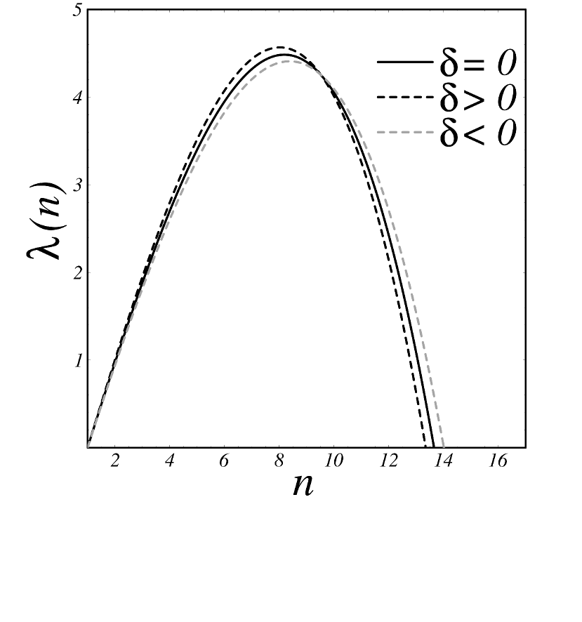
Figure 2: Linear growth rate (28) as a function of mode number $n$ for three different values of the non-Newtoniam parameter: $\delta=0$ (black solid curve), +0.05 (black dashed curve), -0.05 (gray dashed curve). The injection rate $Q=2\pi~{}{\rm cm^{2}/s}$, $R=1~{}{\rm cm}$, and $\gamma=1/200~{}{\rm cm^{3}/s}$. The units of $\lambda(n)$ and $\delta$ are ${\rm s}^{-1}$ and $({\rm cm/s})^{-2}$, respectively.

Our first order results, namely our linear growth rate expression (28), agrees with Kondic et al. Kondic_96 equivalent formula, if we set their constant $C$ equal to ${\dot{R}}^{2}$. We use growth rate (28) to gain insight into shear thinning/thickening behavior. Figure 2 plots $\lambda(n)$ as a function of mode number $n$ for three different values of the non-Newtoniam parameter: a) $\delta=0$; b) $\delta=0.05$; and c) $\delta=-0.05$. By inspecting Fig. 2, we notice that, unlike the shear thinning case ($\delta>0$) discussed in references Kondic_96 ; Kondic_98 , shear thickening ($\delta<0$) widens the band of unstable modes, and decreases growth rate for the wave number of maximal growth. So, by applying similar arguments as those used by Kondic et al. Kondic_96 ; Kondic_98 for the weak shear thinning case, we postulate that shear thickening would lead to enhanced tip-splitting. Unfortunately, for the shear thickening radial Hele-Shaw flow, both numerical simulations and experiments are not available in the literature to confirm this claim. Of course, it is also of interest to study such a possibility analytically. This is one of the topics we examine in Sec. III.2.

III.2 Second order

On the analytical side, one must go beyond linear analysis in order to investigate in more detail the main morphological features found in Hele-Shaw flows with both shear thinning and shear thickening fluids. To this day, besides a few first order linear growth studies Kondic_96 ; Kondic_98 ; Kondic_long , there are no other analytical results concerning non-Newtonian fluid evolution in radial Hele-Shaw geometry. If on one hand the non-Newtonian problem is vastly richer, it is also true it is much less amenable to analytic attack than its Newtonian counterpart. Our mode-coupling approach intends to provide a better and more complete analytical understanding of the complex non-Newtonian time evolution dynamics in Hele-Shaw cells.

III.2.1 Action of the parameter $\delta$ on finger tip-splitting

We use the mode-coupling equation (26) to investigate the coupling of a small number of modes. At second order the most noteworthy effect refers to the action of the non-Newtonian parameter $\delta$ on finger tip-splitting. Tip-splitting is related to the influence of a fundamental mode $n$ on the growth of its harmonic $2n$ MW_rad . For consistent second order expressions, we replace the time derivative terms $\dot{a}_{n}$ and $\dot{b}_{n}$ by $\lambda(n)~{}a_{n}$ and $\lambda(n)~{}b_{n}$, respectively. Under these circumstances the equation of motion for the cosine mode $2n$ is

$$\dot{a}_{2n}=\lambda(2n)~{}a_{2n}+\frac{1}{2}~{}T(2n,n)~{}a_{n}^{2},$$ (32)

where the function that multiplies $a_{n}^{2}$, $T(2n,n)$, is called the tip-splitting function and its general expression is

$$T(n,m) = F_{N}(n,m)+\lambda(m)~{}G_{N}(n,m)+\delta~{}[F_{NN}(n,m)+\lambda(m)~{}G_{NN}(n,m)$$ (33)

$$+ \lambda(n-m)~{}H_{NN}(n,m)+\lambda(m)~{}\lambda(n-m)~{}J_{NN}(n,m)].$$

Equation (32) shows that the presence of the fundamental mode $n$ forces growth of the harmonic mode $2n$. The function $T(2n,n)$ acts like a driving force and its sign dictates if finger tip-splitting is favored or not by the dynamics. If $T(2n,n)<0$, $a_{2n}$ is driven negative, precisely the sign that leads to finger tip-widening and finger tip-splitting. If $T(2n,n)>0$ growth of $a_{2n}>0$ would be favored, leading to outwards-pointing finger tip-narrowing.

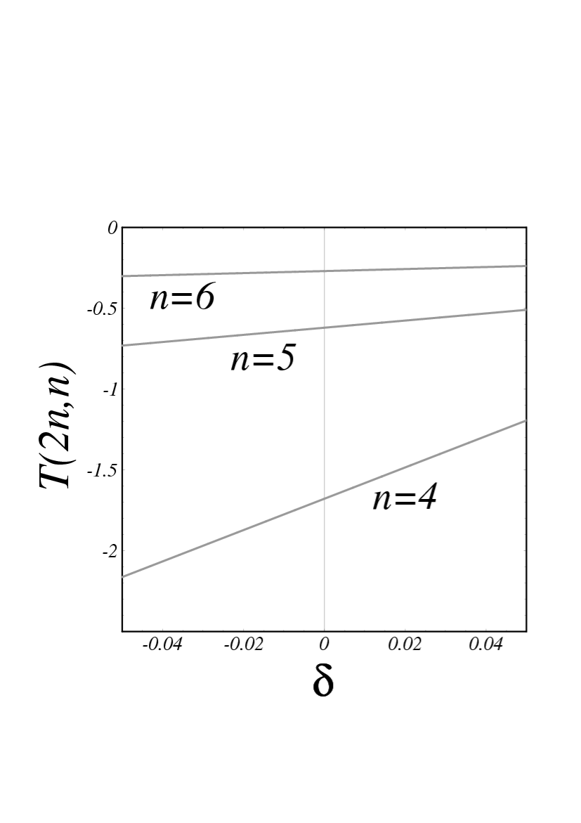
Figure 3: Variation of $T(2n,n)$ as a function of the non-Newtonian parameter $\delta$, for three different Fourier modes ($n=4,5,6$). The injection rate $Q=2\pi~{}{\rm cm^{2}/s}$ and $\gamma=1/100~{}{\rm cm^{3}/s}$. The units of $T(2n,n)$ and $\delta$ are $({\rm cm~{}s})^{-1}$ and $({\rm cm/s})^{-2}$, respectively.

To investigate the influence of the non-Newtonian parameter $\delta$ on tip-splitting behavior at second order, we plot in Fig. 3 the behavior of $T(2n,n)$ as a function of $\delta$, for a few Fourier modes ($n=4,5,6$). To simplify our analysis we adopt an instantaneous approach: we consider a particular ${\dot{R}}$ and $R$ combination, using the identity ${\dot{R}}R=Q/2\pi$, at the onset of growth of mode $2n$ [using the condition $\lambda(2n)=0$] in the Newtonian limit $\delta=0$, where we know $T(2n,n)$ is negative MW_rad . We see from Fig. 3 that the curve for mode $n=4$ lies below the curves associated to $n=5,6$. This is an expected behavior since smaller values of $n$ would mean more room for the existing fingers to split. We also observe that the curves associated to smaller $n$ show a stronger angular inclination with respect to the horizontal $\delta$-axis. Therefore, lower Fourier modes would be more sensitive to variations in $\delta$.

Further inspection of Fig. 3 reveals that, for $\delta>0$, $T(2n,n)$ becomes less negative as $\delta$ increases, meaning that the interface has less tendency toward tip-splitting. In contrast, for $\delta<0$ we observe that $T(2n,n)$ becomes more negative as the magnitude of $\delta<0$ increases, indicating an enhanced tendency of the fingers to split at their tips. We conclude that tip-splitting is suppressed for shear thinning fluids, and enhanced for shear thickening ones. This fact is more clearly illustrated in Fig. 4. In Fig. 4 we plot the fluid-fluid interface for a certain time ($t=30~{}{\rm s}$), considering the interaction of two cosine modes (a fundamental $n=4$ and its harmonic $2n=8$), for three diferrent values of $\delta$: (a) $\delta=0$ (solid curve); (b) $\delta>0$ (black dashed curve); and (c) $\delta<0$ (gray dashed curve). From Fig. 4 it is evident that there is a stronger splitting in the shear thickening case.

These second order effects regarding tip-splitting are consistent with the first order effects described in section III.1. With respect to shear thinning behavior, our analytical results agree with numerical simulations Kondic_98 ; Kondic_long and experiments MW_1b ; Buka of fully nonlinear stages of interface evolution. In addition, we detect favored tip-splitting in the shear thickening case, a relevant nonlinear behavior not previously reported in the literature. We have also verified that, for a given mode $n$, smaller values of the surface tension parameter $\gamma$ lead to enhancement (suppression) of splitting events for $\delta<0$ ($\delta>0$).

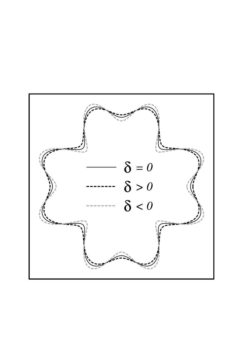
Figure 4: Snapshot of the fluid-fluid interface ($t=30~{}{\rm s}$), for the interaction of two cosine modes $n=4$ and $2n=8$. Three values of the non-Newtonian parameter are considered $\delta=0$ (black solid curve), $\delta=+0.01~{}({\rm cm/s})^{-2}$ (black dashed curve), and $\delta=-0.01~{}({\rm cm/s})^{-2}$ (gray dashed curve). Other physical parameters are: $a_{n}(0)=0.001~{}{\rm cm}$, $R_{0}=0.3~{}{\rm cm}$, $\gamma=0.025~{}{\rm cm^{3}/s}$, and $Q=3\pi~{}{\rm cm^{2}/s}$. Splitting is favored for shear-thickening fluids (gray dashed curve).

A physical mechanism that seems to be at work in shear thinning case has been proposed in references Kondic_96 ; Kondic_98 ; Kondic_long : viscosity is lowered in high-shear regions, which are in front of the fingers. Hence the tip of a finger experiences less resistance than the part of the interface near the tip. This suggests that tip-splitting would be suppressed if the fluid shear-thins. Our second order mode-coupling results indicate that a similar mechanism is at work in the shear thickening case: the resistance would be increased at the finger tips, suggesting that tip-splitting would be increased.

III.2.2 Action of the parameter $\delta$ on side branching

Another relevant non-Newtonian effect that can be studied at second order refers to the side branching phenomenon. In the framework of a mode-coupling theory, side branching requires the presence of mode $3n$. If the harmonic mode $a_{3n}$ is positive and sufficiently large, it can produce interfacial lobes branching out sidewards which we interpret as side branching.

Consider the influence of the fundamental mode $n$, and its harmonic $2n$, on the growth of mode $3n$. The equation of motion for the cosine $3n$ mode is

$$\dot{a}_{3n}=\lambda(3n)~{}a_{3n}+\frac{1}{2}~{}S(3n)~{}a_{n}a_{2n},$$ (34)

where the side branching function $S(3n)=\left[T(3n,n)+T(3n,2n)\right]$ can be easily obtained from Eq. (33). By analyzing Eq. (34) we observe that mode $3n$ can be spontaneously generated due to the driving term proportional to $a_{n}a_{2n}$, such that it enters through the dynamics even when it is missing from the initial conditions. The existence and phase of mode $3n$ depends on the interplay of the modes $n$ and $2n$. Side branching would be favored if $a_{3n}>0$.

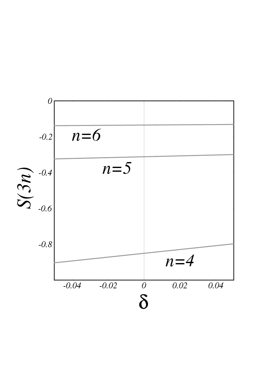
Figure 5: Variation of the side branching function $S(3n)=T(3n,n)+T(3n,2n)$ with the non-Newtonian parameter $\delta$, for modes $n=4,5,6$. The injection rate $Q=2\pi~{}{\rm cm^{2}/s}$ and $\gamma=1/100~{}{\rm cm^{3}/s}$. The units of $S(3n)$ and $\delta$ are $({\rm cm~{}s})^{-1}$ and $({\rm cm/s})^{-2}$, respectively.

To study the growth of mode $3n$ as the non-Newtonian parameter $\delta$ is varied, we plot $S(3n)$ as a function of $\delta$ in Fig. 5. We consider a particular ${\dot{R}}$ and $R$ combination that corresponds to the onset of growth of mode $3n$ (i.e. obeying the condition $\lambda(3n)=0$) in the Newtonian limit $\delta=0$. From Fig. 5 one can verify that in the weak shear limit we consider in this work, $S(3n)$ is negative for all values of $\delta$. As shown in section III.2.1, starting with a fundamental mode $a_{n}$, the harmonic mode $a_{2n}$ is driven negative. Hence the product $S(3n)a_{n}a_{2n}$ in Eq. (34) is positive, driving $a_{3n}>0$.

Whether side branching actually occurs depends on the magnitude of $a_{3n}$. Indeed, our discussion shows the presence of $a_{3n}>0$ even in the case of Newtonian fluids, where side branching does not occur. Why does side branching occur for shear thinning fluids? We speculate its origin may lie in the cubic form of our modified Darcy’s law, Eq. (5), which will add a term of the form $\delta a_{n}^{3}$ to $\dot{a}_{3n}$. Unfortunately, we have not calculated this term since we stopped our derivation at second order. Third order calculations for non-Newtonian Hele-Shaw flows lead to several new and complex mode-coupling terms, whose analysis and interpretation are not at all obvious, and go beyond the scope of our current work

Furthermore, there is a delicate interplay of mode $3n$ and mode $2n$, described by the evolution equation (34) and a similar expression for the growth of mode $2n$,

$$\dot{a}_{2n}=\lambda(2n)~{}a_{2n}+\frac{1}{2}~{}[T(2n,n)~{}a_{n}^{2}+S(2n)~{}a_{n}a_{3n}],$$ (35)

where $S(2n)=[T(2n,-n)+T(2n,3n)]>0$. Hence, side branching via a positive $a_{3n}$ will tend to drive $a_{2n}$ positive (or at least less negative), inhibiting tip splitting but also reducing the growth rate of $a_{3n}$ itself.

III.3 Rectangular geometry limit

It is interesting to study how the main interfacial features examined in the radial geometry behave if we consider flow of non-Newtonian fluids in rectangular Hele-Shaw cells. A mode-coupling equation describing the system can be obtained if we take the “rectangular geometry limit”: $R\rightarrow\infty$ and $Q\rightarrow\infty$, such that $Q/(2\pi R)\equiv v_{\infty}$ and $n/R\equiv k$ remain constant, where $v_{\infty}$ is the flow velocity at infinity and $k$ denotes the wave number of the disturbance. In this limit the interface evolution reverts to the evolution of the rectangular flow geometry, with linear growth rate given by

$$\lambda(k)=|k|\left[v_{\infty}(1+\delta v_{\infty}^{2})-\gamma|k|^{2}(1+2\delta v_{\infty}^{2})\right].$$ (36)

In addition, the only nonzero second order mode-coupling terms are

$$G_{N}(k,k^{\prime})=|k|\left[1-{\rm sgn}(k~{}k^{{}^{\prime}})\right],$$ (37)

$$G_{NN}(k,k^{\prime})=-|k|v_{\infty}^{2}\left[1-{\rm sgn}(k~{}k^{{}^{\prime}})\right],$$ (38)

and

$$J_{NN}(k,k^{\prime})=\frac{v_{\infty}}{2}\left\{3-{\rm sgn}[k^{{}^{\prime}}(k-k^{{}^{\prime}})]+2~{}{\rm sgn}[k(k-k^{{}^{\prime}})]\right\}.$$ (39)

Note that all rectangular limit expressions (36)-(39) are time-independent, and preserve the reflection symmetries shown in Eq. (II). Based on these findings, and using Eq. (26) we obtain a more compact mode-coupling equation for non-Newtonian flow in rectangular Hele-Shaw cells

$${\dot{\zeta}_{k}} = \lambda(k)~{}\zeta_{k}+\sum_{k^{{}^{\prime}}\neq k,0}\left[G_{N}(k,k^{{}^{\prime}})+\delta~{}G_{NN}(k,k^{{}^{\prime}})\right]~{}\dot{\zeta}_{k^{{}^{\prime}}}\zeta_{k-k^{{}^{\prime}}}$$ (40)

$$+ \delta\sum_{k^{{}^{\prime}}\neq k,0}J_{NN}(k,k^{{}^{\prime}})~{}\dot{\zeta}_{k^{{}^{\prime}}}\dot{\zeta}_{k-k^{{}^{\prime}}}.$$

The rectangular mode-coupling Eq. (40) is useful to study the influence of weak shear effects on the development of the fluid-fluid interface in rectangular cells. First, we examine finger tip-splitting related issues (finger narrowing/widening). As discussed in section III.2.1, we analyze the influence of the fundamental $k$ on the growth of its harmonic $2k$. The equation of motion for the cosine mode $2k$ is

$$\dot{a}_{2k}=\lambda(2k)~{}a_{2k}+\frac{1}{2}~{}T(2k,k)~{}a_{k}^{2},$$ (41)

where

$$T(2k,k)=\delta\left[2k^{2}v_{\infty}(v_{\infty}-\gamma~{}k^{2})^{2}\right].$$ (42)

Note that the driving force term $T(2k,k)$ vanishes in the Newtonian limit $\delta=0$. This agrees with the results obtained in Ref. MW_rectang for Newtonian rectangular flow. Notice further, that for the non-Newtonian case ($\delta\neq 0$) the harmonic mode $2k$ grows spontaneously even if missing from the initial conditions. The selected sign of $a_{2k}$ is given by the sign of $T(2k,k)$ and thus is dictated by $\delta$: if $\delta>0$ ($\delta<0$), $T(2k,k)$ is positive (negative), and hence $a_{2k}>0$ ($a_{2k}<0$).

Considering the case $\delta>0$, this means that the fingers become narrower as the shear thinning behavior becomes more pronounced. Moreover, by inspecting Eq. (42) we observe that the width of the finger tips decreases for increasingly larger values of the flow velocity $v_{\infty}$. Of course, these effects are minimized for larger values of the surface tension parameter $\gamma$. All these results are in agreement with recent experimental Lindner and theoretical investigations Ben1 ; Ben2 for weak shear-thinning flows in rectangular geometry, in which shear-thinning narrows the width of steady state fingers.

If we take $k=k^{\star}\approx\sqrt{v_{\infty}/3\gamma}$ as the fastest growing mode, then $\lambda(2k)<0$ so exponential growth of $a_{2k}$ is prevented. Unlike the case of radial flow where any mode $n$ eventually goes unstable for sufficiently large $R$, the growth rates $\lambda(k)$ in the rectangular geometry are time independent. Instead of exponential growth of $a_{2k}$, we instead expect its amplitude to saturate at the value $T(2k,k)a_{k}^{2}/(-2\lambda(2k))$ obtained by setting $\dot{a}_{2k}=0$ in Eq. (41). Alternatively, one could specially prepare an initial condition with an initial perturbation of wavevector $k$ sufficiently small that $2k$ still lies within the band of unstable modes (up to about $\sqrt{v_{\infty}/\gamma}$), in which case mode $2k$ will be spontaneously generated and able to grow to a considerable magnitude.

For completeness, we also discuss the shear thickening case: for $\delta<0$ the function $T(2k,k)$ is negative, favoring finger tip-widening. Even though this shear thickening behavior has not been studied experimentally, the broadening of the fingers in shear thickening flow in rectangular cells has been theoretically predicted by numerical simulations Ben2 . Our analytical results reinforce the correctness of such numerical predictions.

Finally, we briefly discuss side branching behavior in rectangular Hele-Shaw cells. We consider the influence of modes $k$ and $2k$ on the evolution of mode $3k$. In this case, the relevant equation of motion has the form

$$\dot{a}_{3k}=\lambda(3k)~{}a_{3k}+\frac{1}{2}~{}S(3k)~{}a_{k}a_{2k},$$ (43)

where, as it was in the radial flow case, the coefficient $S(3k)$ is the sum of $T(3k,k)$ and $T(3k,2k)$

$$S(3k)=\delta\left[8k^{2}v_{\infty}(v_{\infty}-\gamma~{}k^{2})~{}(v_{\infty}-4\gamma k^{2})\right].$$ (44)

The favored sign of $a_{3k}$ depends on the sign of the product $a_{k}a_{2k}$ and also on the sign of $S(3k)$. If $\delta$ is positive (shear thinning) then $S(3k)$ is negative in the band of wavevectors

$$\sqrt{v_{\infty}/4\gamma}<k<\sqrt{v_{\infty}/\gamma}$$ (45)

and positive outside this band. As we saw previously in the case of mode $2k$, if the fundamental mode is taken as the fastest growing mode $k=k^{\star}$, then exponential growth of the harmonic $3k$ is inhibited because $\lambda(3k)<0$. Instead it will saturate at a magnitude of $S(3k)a_{k}a_{2k}/(-2\lambda(3k))$.

However, for a specially prepared initial condition perturbed at wavevector $k\approx k^{\star}/3$, the harmonics $2k$ and $3k$ will both be able to grow. By Eq. (41) a positive harmonic mode $a_{2k}>0$ will appear spontaneously. Then, by Eq. (43), modes $a_{k}$ and $a_{2k}$ will conspire to create mode $a_{3k}$. Because $k\approx k^{\star}/3$ lies outside the wavevector band (45), the value of $S(3k)$ is positive. Hence the mode $a_{3k}$ is driven positive, the sign needed to create side branches. While this conclusion is only tentative (due to our neglect of the complete set of third order terms) it would be interesting to test via numerical simulation or experiment.

IV Concluding remarks

Visually striking patterns arise when a less viscous Newtonian fluid displaces a more viscous non-Newtonian fluid in the confined geometry of a Hele-Shaw cell. These complex patterned structures are the result of finger tip-splitting and dendritic interfacial instabilities. Due to the complicated dynamics of the system, and also from the limitations imposed by purely linear analysis, the majority of the theoretical studies in this area of research rely heavily on sophisticated numerical methods. In this work, we developed an alternative theoretical approach to the problem which allowed us to address important nonlinear issues analytically. A key point in our derivation was the introduction of velocity vector potential (as opposed to scalar potential) which was demanded by the non-Newtonian fluid flow.

We started our investigation by analyzing the role of fluid viscosity anisotropy on the development of the Saffman-Taylor instability in radial Hele-Shaw cells. To approach the problem analytically we considered the weak shear limit, and focused on the onset of nonlinear effects. In order to examine the influence of shear thinning and shear thickening on the shape of the emerging patterns, we derived a mode-coupling equation which is ideally suited to describe the weakly nonlinear interface evolution. Our analytical results show that finger tip-splitting is enhanced (diminished) in the case of shear thickening (thinning) fluids. We applied the rectangular geometry limit to our radial mode-coupling equations of motion, and also studied finger-tip and side branching behavior in rectangular cells. Our main findings predict finger tip-widening (narrowing) for shear thickening (thinning) fluids.

In neither the radial nor the rectangular geometry limit were we able to show the spontaneous appearance of side branching, except for some specially prepared initial conditions in rectangular geometry. We speculate that extending the current approach to third order could shed more light on this problem.

In summary, our analytical mode-coupling approach detects and predicts several features of the patterns formed in non-Newtonian Hele-Shaw flows in both radial and rectangular geometries. Furthermore, it predicts some behaviors not yet investigated in the literature, such as the evolution mechanisms involving tendency towards advanced finger tip-splitting and reduction of side branching for shear thickening fluids. We hope the main results presented in this paper will prompt further theoretical and experimental work on non-Newtonian Hele-Shaw flows, especially in the area of early stage transients in rectangular geometry where our theory makes specific predictions that have not been subject to experimental or numerical check.

*

Appendix A Second order mode-coupling terms

This appendix presents the expressions for the second order Newtonian (N), and non-Newtonian (NN) mode-coupling coefficients which appear in Eq. (29)

$${F_{N}\left(n,m\right)}=\frac{|n|}{R}\left\{\frac{{\dot{R}}}{R}\left[\frac{1}{2}-{\rm sgn}(nm)\right]-\frac{\gamma}{R^{3}}\left(1-\frac{nm}{2}-\frac{3m^{2}}{2}\right)\right\},$$ (46)

$$F_{NN}(n,m) = \frac{|n|}{R}{\dot{R}}^{2}\Bigg{\{}\frac{{\dot{R}}}{R}\left[\frac{2\alpha(m)}{m}\frac{|n|}{n}-\frac{2\beta(n)}{|n|}+\frac{f(n,m)}{2(|n|+1)}\right]$$ (47)

$$- \frac{\gamma}{R^{3}}\frac{2|n|}{(|n|+1)}\left(1-\frac{nm}{2}-\frac{3m^{2}}{2}\right)\Bigg{\}},$$

$$G_{N}\left(n,m\right)=\frac{|n|}{R}\left[1-{\rm sgn}(nm)-\frac{1}{|n|}\right],$$ (48)

$$G_{NN}\left(n,m\right)=\frac{|n|}{R}{\dot{R}}^{2}\left[\frac{2\alpha(m)}{m}\frac{|n|}{n}-\frac{2\beta(n)}{|n|}+\frac{f(n,m)}{2(|n|+1)}\right],$$ (49)

$$H_{NN}\left(n,m\right)=\frac{|n|}{2(|n|+1)}\frac{{\dot{R}}^{2}}{R}~{}f(n,m),$$ (50)

and

$$J_{NN}\left(n,m\right)=\frac{|n|}{2(|n|+1)}{\dot{R}}~{}f(n,m),$$ (51)

where

$$f(n,m)=\left[\frac{|n|}{n}h\left(n,m\right)+k\left(n,m\right)\right].$$ (52)

References

- (1) P. G. Saffman and G. I. Taylor, Proc. Roy. Soc. London Ser. A245, 312 (1958).
- (2) L. Paterson, J. Fluid Mech. 113, 513 (1981).
- (3) B. Bensimon, L. P. Kadanoff, S. Liang, B. I. Shraiman, and C. Tang, Rev. Mod. Phys. 58, 997 (1986).
- (4) K. V. McCloud and J. V. Maher, Phys. Rep. 260, 139 (1995).
- (5) H. Van Damme, E. Lemaire, O. M. Abdelhaye, A. Mourchid, and P. Levitz, Non-linearity and Breakdown in Soft Condensed Matter, edited by K. K. Bardan et al., Lecture Notes in Physics Vol. 437, (Springer, New York, 1994).
- (6) A. Buka, P. Palffy-Muhoray, and Z. Racz, Phys. Rev. A 36, 3984 (1987).
- (7) E Lemaire, P. Levitz, G. Daccord, and H. Van Damme, Phys. Rev. Lett. 67, 2009 (1991).
- (8) H. Zhao and J. V. Maher, Phys. Rev. E 47, 4278 (1993).
- (9) J. E. Sader, D. Y. C. Chan, and B. D. Hughes, Phys. Rev. E 49, 420 (1994).
- (10) D. Bonn, H. Kellay, M. Ben Amar and J. Meunier, Phys. Rev. Lett. 75, 2132 (1995); D. Bonn, H. Kellay, M. Braunlich, M. Ben Amar, and J. Meunier, Physica A 220, 60 (1995).
- (11) L. Kondic, P. Palffy-Muhoray, and M. J. Shelley, Phys. Rev. E 54, R4536 (1996).
- (12) L. Kondic, M. J. Shelley, and P. Palffy-Muhoray, Phys. Rev. Lett. 80, 1433 (1998).
- (13) P. Fast, L. Kondic, M. J. Shelley, and P. Palffy-Muhoray, Phys. Fluids 13, 1191 (2001).
- (14) J. A. Miranda and M. Widom, Int. J. Mod. Phys. B 12, 931 (1998).
- (15) J. A. Miranda and M. Widom, Physica D 120, 315 (1998).
- (16) A. Lindner, D. Bonn, and J. Meunier, Phys. Fluids 12, 256 (2000).
- (17) E. Corvera Poiré and M. Ben Amar, Phys. Rev. Lett. 81, 2048 (1998).
- (18) M. Ben Amar and E. Corvera Poiré, Phys. Fluids 11, 1757 (1999).