Generating correlated networks from uncorrelated ones

Abstract

In this paper we consider a transformation which converts uncorrelated networks to correlated ones( here by correlation we mean that coordination numbers of two neighbors are not independent). We show that this transformation, which converts edges to nodes and connects them according to a deterministic rule, nearly preserves the degree distribution of the network and significantly increases the clustering coefficient. This transformation also enables us to relate percolation properties of the two networks.

I Introduction

One of the oldest and best studied models of networks which have the merit of being exactly solvable for many of their properties, are the random graphs of Erdös and Rényi er ; b . These graphs consist of $N$ nodes any two of which are connected with a probability $p$ and left unconnected with a probability $1-p$. Many of the properties of these networks can be easily derived by analytical means. Among them are the degree distribution of nodes, which turns out to be Poissonian, the average shortest path between any two nodes which is of the order of $\log(N)$, and the onset of phase transition for developing a giant component which happens as $p$ exceeds a certain critical value.
Despite their exact solvability and their low diameter, these networks lack some of the other crucial properties of real life networks. In particular it is well known that many real networks e.g. World Wide Web, social networks, power grids, scientific and artistic collaborations, neural and metabolic networks, show clustering or transitivity which is absent in Erdös and Rényi graphs. Moreover many real networks do not possess Poissonian degree distribution and intensive studies have been made to construct models as close as to real networks ab ; s ; ws ; dm and to study dynamic effects, e.g. spreading of a contact effect, on them.ka ; pv .
In the past few years an elegant theory has been developed to construct random graphs with desirable degree distributions to mimic the degree properties of real networks. It appears that Bender and Canfield bc ; nsw have been the first to propose an algorithm for constructing a random graph with a specific degree distribution. We will call the ensemble of graphs constructed in this way the Bender Canfield ensemble. It is remarkable that these graphs are still exactly solvable to a large extent nsw . However these graphs still have two shortcomings. First they do not show correlation in the degree of nearest neighbors and second their clustering coefficient vanishes in the large $N$ limit.
It is important that the degree distribution does not determine by itself the existence or lack of correlations. For a specific degree distribution one may have or have not correlations. Moreover, it has been observed that correlation is an essential feature of real networks which can appear in different forms n . For instance, a high degree node may be connected to other high degree nodes(associative mixing), to low degree nodes(dissociative mixing) or with equal probability to both types (neutral mixing) with different resulting behaviors in networks bp ; mnl ; kr ; pvv .
For this reason algorithms have been developed to produce correlated networks with certain degree distribution dms1 ; bl ; n ; dm .

In this paper we will suggest a simple deterministic transformation on the Bender Canfield (BC) graphs and show that the transformed graphs are both correlated and clustered in the large $N$ limit. Given a BC graph $G$ with $N$ nodes and a degree distribution $P(k)$, we construct a graph $\tilde{G}$ by assigning nodes to each edge of $G$. We then connect these new nodes if the corresponding edges in $G$ have had a common node in $G$. We show that many of the properties of these transformed networks can be obtained exactly or almost exactly. We obtain general formulas for the degree distribution and its correlations for the transformed graphs and will obtain also formulas for the clustering coefficients of these new graphs. As examples we apply our transformation to Bender Canfield graphs with various degree distributions.
It has been shown by Newman that percolation on BC graphs can be solved by a generating function method. The method is applicable due to the fact that in these graphs there is no clustering. By applying our transformation to these graphs we can follow similar steps and solve percolation on $\tilde{G}$ . The interesting point is that now $\tilde{G}$ is a highly clustered graph for which we can solve percolation.
The paper is structured as follows: In section II we give a brief review of Bender Canfield ensemble of random graphs having arbitrary degree distributions. In section III we discuss our transformation and derive various properties of general transformed graphs. In section IV we apply our general formulas to graphs with degree distributions of Poissonian, scale free and exponential types. We end the paper with a conclusion.

II Bender-Canfield ensemble of graphs

Let $G$ denote a graph with $N$ edges and $L$ links. Let also the degree distribution of this graph be given by the function $P(k)$, that is the fraction of nodes with $k$ neighbors be given by $P(k)$. There is an algorithm bc ; nsw for constructing graphs whose degree distribution corresponds to $P(k)$ for large $N$. More specifically given a degree sequence $(k_{1},k_{2},\cdots k_{N})$ corresponding to the desired degree distribution $P(k)$, one takes each node $i$ with $k_{i}$ loose ends (stubs) and then connects each pair of stubs randomly until no loose end remains. We call these types of graphs Bender-Canfield or simply BC graphs. Thus we speak of Poissonian BC graphs or scale free BC graphs to designate the degree distribution used for their construction.
Many of the properties of BC graphs can be calculated exactly. For example the average number of first neighbors of an arbitrary node, denoted by $z_{1}$ is given by

$$z_{1}:=\langle k\rangle=\sum_{k}kP(k).$$ (1)

It is useful to call a node with $k$ emanating edges a node of type $k$. Then the probability of picking up a node of type $k$ is given by $P(k)$. We can now ask a different question: What is the probability $q(k)$ of picking up an edge which belongs to a node of type $k+1$. This is equal to the fraction of stubs coming out of nodes of type $k+1$:

$$q(k)=\frac{(k+1)P(k+1)}{\sum_{k}kP(k)}\equiv\frac{(k+1)P(k+1)}{\langle k\rangle}$$ (2)

If we now follow a link to one of its ends the average number of new links ( the average ratio of the number of second to the first neighbors of an arbitrary node $\frac{z_{2}}{z_{1}}$) will be given by

$$\frac{z_{2}}{z_{1}}=\sum_{k}kq(k)=\frac{\langle k^{2}\rangle-\langle k\rangle.}{\langle k\rangle}$$ (3)

As we will see this quantity will play a central role in many of the later derivations.

We can ask yet another question. What is the probability $P(k,k^{\prime})$ of picking up an edge which is common to a node of type $k+1$ and a node of type $k^{\prime}+1$?. This probability is given by a product which is a reflection of the absence of correlations in these networks,

$$P(k,k^{\prime})=q(k)q(k^{\prime}).$$ (4)

One can also calculate the clustering coefficient of these graphs. The result is nsw

$$C=\frac{z_{1}}{N}(\frac{\langle k^{2}\rangle-\langle k\rangle}{\langle k\rangle^{2}})^{2}=\frac{1}{n}\frac{(z_{2})^{2}}{(z_{1})^{3}}.$$ (5)

It is important to note that for many kinds of degree distributions (i.e. those with finite $z_{2}$ and $z_{1}$), this clustering coefficient vanishes in the limit of large graph size $N$. It can also be shown that the ratio $\frac{z_{2}}{z_{1}}$ controls the existence of an infinite cluster of connected nodes nsw ; dms2 for these graphs. For $\frac{z_{2}}{z_{1}}>1$ there is an infinite cluster where the average distance between two arbitrary nodes, is of order $log(n)$. Recently it has been found that almost all pairs of nodes have the same distance in this cluster dms2 .
It will be convenient to define two generating functions for the BC ensemble corresponding to a degree distribution:

$$G_{0}(t):=\sum_{k}t^{k}P(k)\hskip 56.9055ptG_{1}(t):=\sum_{k}t^{k}q(k)=\frac{1}{z_{1}}G_{0}^{\prime}(t)$$ (6)

where $G^{\prime}(t)=\frac{d}{dt}G(t)$ and in the last relation we have used (2). In terms of these generating functions, the average number of first neighbors $z_{1}$ and second neighbors $z_{2}$ are simply given by

$$z_{1}=\frac{d}{dt}G_{0}(t)|_{t=1}\hskip 56.9055ptz_{2}=z_{1}\frac{d}{dt}G_{1}(t)|_{t=1}=G_{0}^{\prime\prime}(1).$$ (7)

III Transformation of BC graphs

Consider a BC graph $G$ with $N$ nodes with a degree sequence $(k_{1},k_{2},\cdots k_{N})$ taken from a distribution $P(k)$. We can transform this graph to a new graph $\tilde{G}$ as follows. To each link of the original graph, we assign a node of the new graph. We connect any two nodes of the new graph if the corresponding links in the original graph have a node in common, see fig.(1). The number of nodes and links of $\tilde{G}$ denoted respectively by $\tilde{N}$ and $\tilde{L}$ respectively are determined from the degree distribution of $G$. We note that each node of type $k$ of $G$ contributes $k$ nodes and $k(k-1)/2$ edges to $\tilde{G}$. Taking care of the fact that the new nodes are counted twice we find:

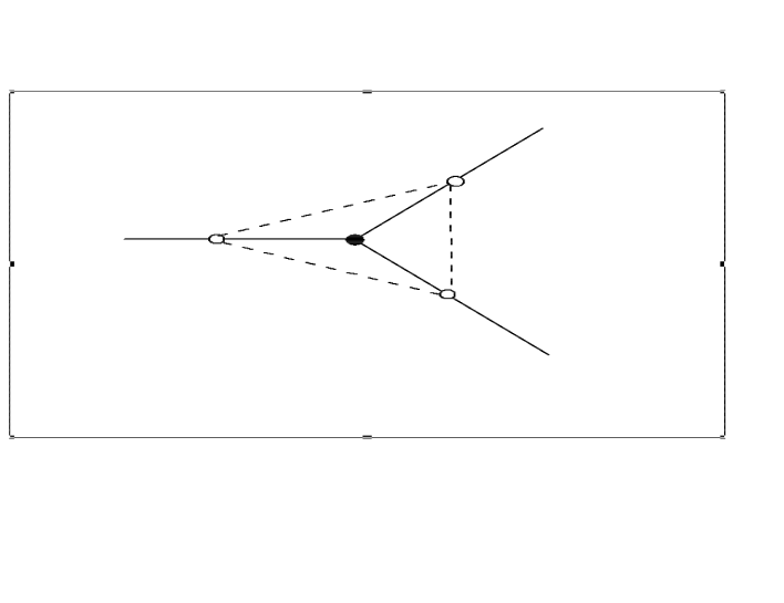
Figure 1: The basic transformation. The filled circle and solid lines belong to $G$ and empty circles and dashed lines belong to $\tilde{G}$.

$$\tilde{N} = \frac{1}{2}\sum_{i=1}^{N}k_{i}$$ (8)

$$\tilde{L} = \frac{1}{2}\sum_{i=1}^{N}k_{i}(k_{i}-1)$$

As figure (2-a) shows the degree distribution of the new graph $\tilde{G}$ is given by:

$$\tilde{P}(k)=\sum_{r+s=k}q(r)q(s),$$ (9)

which is nothing but the probability that an arbitrary edge in $G$ is connected to a total of $k$ edges at its two end point nodes.
There are simple relations between the generating functions of $G$ and $\tilde{G}$. Using (9) we find:

$$\tilde{G_{0}}(t)=\sum_{k}t^{k}\tilde{P}(k)=\sum_{k}t^{k}\sum_{r+s=k}q(r)q(s)=\sum_{r,s}t^{r+s}q(r)q(s)=(\frac{G_{0}^{\prime}(t)}{z_{1}})^{2}$$ (10)

From this last equation we find

$$\tilde{z_{1}}:=\frac{d}{dt}\tilde{G_{0}}(t)|_{t=1}=2\frac{\langle k^{2}-k\rangle}{\langle k\rangle}=2\frac{z_{2}}{z_{1}}$$ (11)

In view of (6) we have

$$\tilde{G_{1}}(t):=\frac{1}{\tilde{z_{1}}}\frac{d}{dt}\tilde{G_{0}}(t)=\frac{G_{0}^{\prime}(t)G_{0}^{\prime\prime}(t)}{z_{1}z_{2}}.$$ (12)

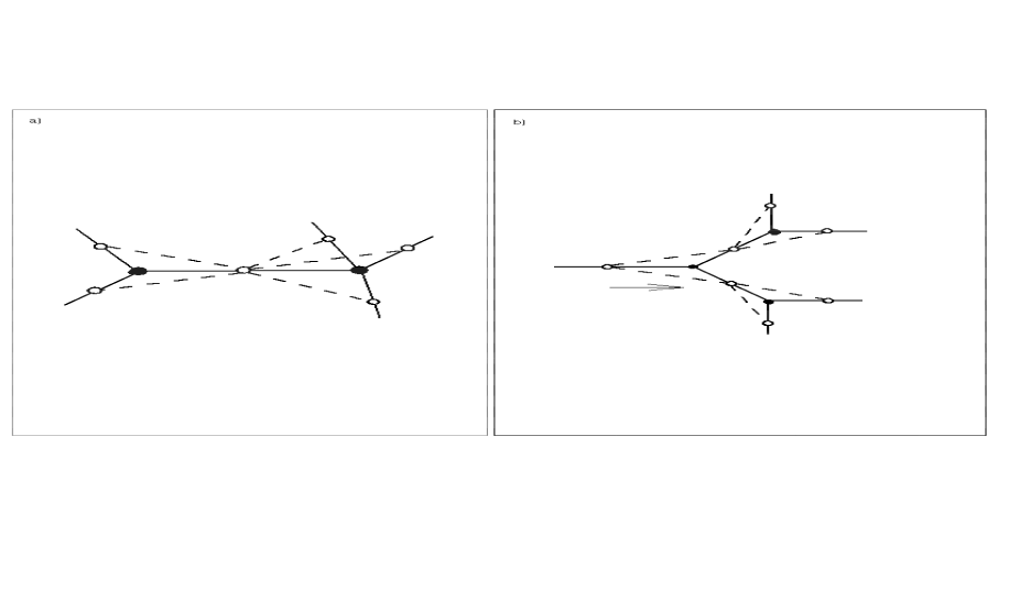
Figure 2: a) First neighbors of a node in $\tilde{G}$. b) Second neighbors of a node in $\tilde{G}$( reachable from one of its sides).

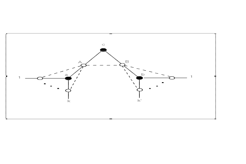
Figure 3: The degrees of the nodes $A$ and $B$ in $\tilde{G}$ are correlated by the vertex $c$ in $G$.

However since the graph $\tilde{G}$ is a clustered graph as we will see, the ratio of average number of second to first neighbors of an arbitrary node, $\frac{\tilde{z_{2}}}{\tilde{z_{1}}}$ is not given by the expression $\sum_{k}k\tilde{q}(k)$ as in (3). Instead we resort to a direct counting. As shown in fig. (2-b) if we follow a node of $\tilde{G}$ to the right, the number of first neighbors that we find is given by $\frac{z_{2}}{z_{1}}$ inherited from $G$. Due to the low clustering of $G$, the number of second neighbors that we will meet will be $(\frac{z_{2}}{z_{1}})^{2}$. Thus the total number of second neighbors will be twice this value, that is $\tilde{z_{2}}=2(\frac{z_{2}}{z_{1}})^{2}$. The above reasoning indeed shows that $\frac{\tilde{z_{2}}}{\tilde{z_{1}}}=\frac{z_{2}}{z_{1}}$ which in turn means that the conditions nsw for the development of a giant component in $G$ and$\tilde{G}$ are identical.
We now find the probability $\tilde{P}(k,k^{\prime})$ of finding an edge the end nodes of which have $k$ and $k^{\prime}$ other neighbors.
Looking at figure (3), the probability of finding an edge like $AB$ in $\tilde{G}$ is equivalent to finding two edges $ac$ and $bc$ incident on the same node $c$ in $G$. For a moment suppose that no other edge in $G$ is incident on $c$. Then it is clear from figure (3) that the nodes $A$ and $B$ will have $k+1$ and $k^{\prime}+1$ neighbors in $\tilde{G}$ if the nodes $a$ and $b$ will have $k+1$ and $k^{\prime}+1$ neighbors in $G$ respectively. Putting this together we find that in this simple case $\tilde{P}(k,k^{\prime})=P(2)q(k)q(k^{\prime})$, where $P(2)$ comes from the probability of finding a node like $c$ of degree $2$ in $G$. In general the node $c$ may be common to $t$ other edges in $G$. These extra edges contribute to the total number of neighbors of $A$ and $B$, so that in order for the node $A$ to have a total of $k+1$ neighbors in $\tilde{G}$, the node $a$ needs only have $k+1-t$ neighbors in $G$. A similar statement is true also for the node $B$. Thus instead of the factor $q(k)q(k^{\prime})$ we will have $q(k-t)q(k^{\prime}-t)$. This should be multiplied by the probability of finding a triplet $acb$ which is proportional to $\frac{(t+2)(t+1)}{2}P(t+2)$ and finally summed over $t$. The final result is

$$\tilde{P}(k,k^{\prime})=\sum_{t}\frac{(t+2)(t+1)}{z_{2}}P(t+2)q(k-t)q(k^{\prime}-t),$$ (13)

In this way correlations are introduced into the graph in the sense that $P(k,k^{\prime})$ is no longer equal to $q(k)q(k^{\prime})$.
It is also possible to calculate the clustering coefficient of $\tilde{G}$. It is clear that an edge with end point nodes of degree $r+1$ and $s+1$ in $G$ represents a node of degree $r+s$ in $\tilde{G}$. Thus the total number of potential connections among these first neighbors is $\frac{(r+s)(r+s-1)}{2}$. Of these possible connections , there are already a number of $\frac{r(r-1)}{2}+\frac{s(s-1)}{2}$ connections present coming from the definition of $\tilde{G}$. Due to the clustering coefficient of $G$, there are configurations which increase this number for finite graphs. However since in the thermodynamic limit we know that the BC graphs have vanishing clustering coefficients we need not worry about these contributions. Thus in the thermodynamic limit we have the following formula for clustering coefficient of $\tilde{G}$:

$$C=\sum_{r,s}\frac{r(r-1)+s(s-1)}{(r+s)(r+s-1)}q(r)q(s).$$ (14)

In this way our transformation has introduced a finite clustering coefficient into the BC ensemble of graphs. In the next section we will apply this transformation to several well known ensembles with specific degree distributions, namely the Poisson, scale free and exponential ensembles.

Finally let us consider percolation on $\tilde{G}$. For the sake of simplicity, here we consider only site percolation but the same analysis can be applied to bond percolation as well. Let each node of $\tilde{G}$ be occupied with probability $p$ and denote the probability that an arbitrary node belongs to a cluster of size $n$, by $P_{n}$. The generating function of this probability is denoted by $H(x)$, that is $H(x)=\sum_{n=0}^{\infty}P_{n}x^{n}$. Using the same procedure as in cnsw we write the following expression for $H(x)$ :

$$H(x)=1-p+pxh^{2}(x),$$ (15)

where $h(x)$ is the generating function for the number of nodes reachable if we follow the neighbors of the node in one of its sides say to the right (i.e. if we follow the corresponding link on $G$ to the right) (see fig. (2-b)). The expression for $h(x)$ is obtained recursively as

$$h(x) = \sum_{k=0}^{\infty}q(k)\sum_{r=0}^{k}(\begin{array}[]{c}k\\ r\end{array})p^{r}(1-p)^{k-r}h^{r}(x)x^{r}$$ (18)

$$= G_{1}(xph(x)+1-p)$$ (19)

Solution of these two equations will give us the probabilities $P_{n}$.

IV Examples

IV.1 Poisson graphs

For a poissonian distribution, where $P(k)=\frac{\lambda^{k}}{k!}e^{-\lambda}$, it is readily verified using () that $q(k)=p(k)$. We find from (9) that

$$\tilde{P}(k)=\sum_{r}P(r)P(k-r)=\frac{\lambda^{r}}{r!}e^{-\lambda}\frac{\lambda^{(k-r)}}{(k-r)!}e^{-\lambda}=\frac{(2\lambda)^{k}}{k!}e^{-2\lambda}$$ (20)

where in the last step we have used the binomial distribution. Thus our transformation maps a poissonian graph to another poissonian graph, whose average degree is twice the original one. However this new graph is completely different from the original one in other respects. First there is correlations between the degree of neighbors and second it has a finite clustering coefficient even for large graphs (as $N\longrightarrow\infty$). To see this we use (13) to calculate for the specific case of $k=k^{\prime}$, the difference $D(k):=\tilde{P}(k,k)-\tilde{q}(k)\tilde{q}(k)$ as a function of $k$ for various values of $\lambda$. The result is shown in fig. (4-a). Figure (4-b) shows the clustering coefficient (calculated from (14)) as a function of $\lambda$. It is clearly seen in this and the other cases considered below that there are non-vanishing correlations in the degree distributions. Also these transformed graphs have appreciable value of clustering. Moreover it is seen that the clustering coefficient approaches a maximum value of nearly $0.5$ for large value of average connectivity. The reason is that, in this limit an appreciable fraction of the nodes of $G$ have a high degree approximately equal to $z_{1}$, and thus one can estimate $C$ from (14) as $C\sim\frac{2z_{1}(z_{1}-1)}{2z_{1}(2z_{1}-1)}\sim 0.5$. This explanation applies to the other examples discussed below.

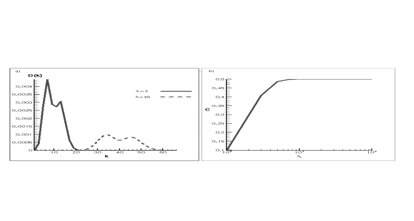
Figure 4: a) plots of $D(k)$ for several values of $\lambda$(here $k_{max}=1000$) and b) Clustering coefficient.

IV.2 Scale free graphs

For scale free graphs we have $P(k)=\frac{1}{\zeta(\gamma)}k^{-\gamma}$ where $\zeta(\gamma)=\sum_{k=1}^{\infty}k^{-\gamma}$. From (1,2) we find $z_{1}=\frac{\zeta(\gamma-1)}{\zeta(\gamma)}$ and $q(k)=\frac{(k+1)^{1-\gamma}}{\zeta(\gamma-1)}$. We find from (9):

$$\tilde{P}(k)=\frac{1}{\zeta^{2}(\gamma-1)}\sum_{s=0}^{k}((s+1)(k+1-s))^{1-\gamma}$$ (21)

It is seen that for $k\gg 1$ the above sum is dominated by its first and last terms. Thus for large $k$, $\tilde{P}(k)$ behaves like $k^{1-\gamma}$ which in turn gives $\tilde{\gamma}=\gamma-1$. Thus the transformation maintains the power law behavior of degree distribution for large degrees. To see this behavior more precisely, we go to the continuum limit and convert the above sum into an integral which after a little rearrangement can be cast into the form:

$$\tilde{P}(k)=(\gamma-2)^{2}\int_{0}^{k}dx[(\frac{k}{2}+1)^{2}-(x-\frac{k}{2})^{2}]^{1-\gamma}$$ (22)

A change of variable $x-\frac{k}{2}=(\frac{k}{2}+1)\sin\theta$ turns this integral into the form

$$\tilde{P}(k)=2(\gamma-2)^{2}(\frac{k}{2}+1)^{3-2\gamma}\int_{0}^{\alpha}{\cos\theta}^{3-2\gamma}d\theta$$ (23)

where $\sin\alpha=\frac{k}{k+2}$. As an example for the case $\gamma=5/2$ we find

$$\tilde{P}(k)=\frac{k}{(k+2)^{2}\sqrt{k+1}},$$ (24)

which as expected, behaves like $k^{-\frac{3}{2}}$ for large $k$. Like the previous example, we calculated numerically $D(k)$ and $C$. The results have been shown in figure (5).

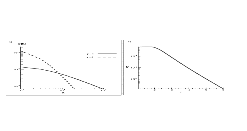
Figure 5: a) $D(k)$ and b) C for scale free graphs.

IV.3 Exponential graphs

Finally, let us consider exponential distributions, $P(k)=Ae^{-\frac{k}{k_{0}}}$ where $A=1-e^{-\frac{1}{k_{0}}}$ is a normalizing factor. We find from (2) $q(k)=\frac{A^{2}}{1-A}(k+1)e^{-\frac{k+1}{k_{0}}}$. Using (9) we find

$$\tilde{P}(k)=\frac{A^{4}}{(1-A)^{2}}e^{-\frac{k+2}{k_{0}}}\sum_{s=0}^{k}(s+1)(k+1-s).$$ (25)

Converting the sum to integral, we find:

$$\tilde{P(k)}=\frac{A^{4}}{(1-A)^{2}}e^{-\frac{k+2}{k_{0}}}(\frac{k^{3}}{6}+k^{2}+k).$$ (26)

We see that transformation does not change the cutoff value, $k_{0}$, but produces some polynomial terms.

In figure (6) we display the correlation and the clustering coefficient for this type of degree distribution, using equations (13) and (14).

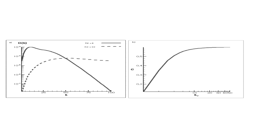
Figure 6: a)$D(k)$ and b)C for exponential degree distribution.

V Conclusion

We have introduced a transformation which when applied to an uncorrelated network with low clustering, produces a new correlated network with a considerable clustering. The small world property of the graph is not affected by this transformation, since the shortest path on two nodes of $G$ is almost the same as the shortest path on two incident links on these nodes on $G$ or two nodes on $\tilde{G}$. We thus have a method to produce ensemble of graphs which resemble more closely the real networks while still being solvable in many respects. Moreover it will be possible to use this transformation and solve dynamic processes on these new graphs. For example we have shown how site percolation can be solved on these transformed graphs.

This transformation can also be applied to already correlated networks. Moreover we have considered only the deterministic form of the transformation . In some cases it may be useful to introduce a stochastic parameter in the transformation to have more degree of freedom. That is the nodes of the transformed graph $\tilde{G}$, can be connected with a probability $p$ if the corresponding edges in $G$ have a common node.
We hope to investigate these issues in subsequent works.

References

- (1) P.Erdös and A.Rényi, Publ. Math. Inst. Hung. Acad. Sci., 5,17 (1960).
- (2) B.Bollobas, 1985, Random Graphs( London: Academic Press).
- (3) R. Albert and A.-L.Barabasi, Rev. Mod. Phys. 74,47-97 (2002).
- (4) S.H.Strogatz, Nature 410, 268-276 (2001).
- (5) D.J.Watts and S.H.Strogatz , Nature 393,440 (1998).
- (6) S.N.Dorogovtsev and J.F.F.Mendes, Advances in Physics 51, 1079-1187 (2002).
- (7) M.Kuperman and G.Abramson,Phys. Rev. Lett. 86, 2909 (2001).
- (8) R.Pastor-Satorras and A.Vespignani, Phys. Rev. E 63, 066117 (2001).
- (9) E.A.Bender and E.R.Canfield, Journal of Combinatorial Theory A 24, 296-307, (1978).
- (10) M.E.J.Newman, S.H.Strogatz and D.J.Watts, Phys. Rev. E 64, 026118 (2001).
- (11) M.E.J. Newman, cond-mat/0209450.
- (12) M.Boguñá and R.Pastor-Satorras, cond-mat/0205621.
- (13) A.E.Motter, T.Nishikawa and Y.-C.Lai, cond-mat/0206030.
- (14) V.Karimipour and A.Ramzanpour, Phys. Rev. E 65 36122 (2002).
- (15) R.Pastor-Satorras, A.Vazquez and A.Vespignani, Phys. Rev. Lett. 87, 258701 (2001).
- (16) S.N.Dorogovtsev, J.F.F.Mendes and A.N.Samukhin, cond-mat/0206131.
- (17) J.Berg and M.Lässing, cond-mat/0205589.
- (18) S.N.Dorogovtsev, J.F.F.Mendes and A.N.Samukhin, cond-mat/0210085.
- (19) D.S.Callaway,M.E.J.Newman, S.H.Strogatz and D.J.Watts, Phys. Rev. Lett. 85, 5468-5471 (2000).