Anomalous behavior of
ideal Fermi gas below two dimensions

Abstract

Normal behavior of the thermodynamic properties of a Fermi gas in $d>2$ dimensions, integer or not, means monotonically increasing or decreasing of its specific heat, chemical potential or isothermal sound velocity, all as functions of temperature. However, for $0<d<2$ dimensions these properties develop a “hump” (or “trough”) which increases (or deepens) as $d\rightarrow 0$. Though not the phase transition signaled by the sharp features (“cusp” or “jump”) in those properties for the ideal Bose gas in $d>2$ (known as the Bose-Einstein condensation), it is nevertheless an intriguing structural anomaly which we exhibit in detail.

PACS: 71.10.Pm; 05.30.Fk; 05.70.Ce; 71.10.-w; 71.10.Ca

Keywords: Electron gas, Fermi gas, low dimension

1 Introduction

The familiar ideal Fermi gas is revisited for any positive space dimension, $d>0$. Ideal Fermi gases (IFG) have been discussed thoroughly in general by several authors [1]-[4] and a detailed study of the quantum behavior in any dimension at sufficiently low temperatures in these systems have also gained interest as possible precursors of a paired-fermion condensate at lower temperatures, these have been studied experimentally in ultra-cold fermionic clouds, e.g., with ${}_{19}^{40}$K neutral atoms in opto-magnetic traps [5]-[8]. From the thermodynamic grand potential we generalize the system to any dimension, we calculated the thermodynamics properties and analyzed the results for the chemical potential, the heat capacity and the isothermal velocity of sound where we found that there are structure if $d<2$ in contrast with the ideal Boson gas where there is structure if $d>2$ [9, 10]. In Sec. 2, we calculate the thermodynamic grand potential for the non-interacting Fermi gas in $d$-dimensions, we find the thermodynamic properties of these systems and deduce a generalized density of states (DOS). In Sec. 3, we calculate the chemical potential $\mu(T),$ the internal energy and the specific heat as function of absolute temperature $T$  for any positive space dimension $d$ and analyzed the results obtained for $d<2$. In Sec. 4 we obtain the isothermal and adiabatic velocities of sound for these systems. Sec. 5 contains our conclusions.

2 Ideal Fermi gas in $d>0$ dimensions

We consider an ideal quantum gas of  fermions in $d>0$ dimensions of mass $m$ in vacuum with a quadratic dispersion relation. The Hamiltonian is then $H=\sum_{i=1}^{d}p_{i}^{2}{/2m}$, its eigenvalues are given by

$$\varepsilon_{n}={\frac{2\pi^{2}\hbar^{2}}{mL^{2}}}\sum_{i=1}^{d}n_{i}^{2},$$ (1)

where $L$ is the size of the “box”, $\mathbf{n}=(n_{1},n_{2},...,n_{d})$, and where $n_{i}=0,\ \pm 1,\;\pm 2,\;...$. Since $k_{i}\equiv(2\pi/L)n_{i}$, (1) can then be rewritten as

$$\varepsilon_{k_{i}}={\frac{\hbar^{2}}{2m}}\sum_{i=1}^{d}k_{i}^{2}.$$ (2)

The thermodynamical properties of this system follow from the thermodynamic (or grand potential) $\Omega(T,L^{d},\mu)=U-TS+\mu N,$ where $U$ is the internal energy, $T$ the absolute temperature, $S$ the entropy, $\mu$ the chemical potential, and $N$ the number of particles. We may write $\Omega(T,L^{d},\mu)$ in generalized form as (see p. 134 of [1])

$$\Omega(T,L^{d},\mu)=-k_{B}T\sum_{{k_{i}}}\hbox{ln}[1+{\normalsize e}^{-{\normalsize\beta}({\normalsize\varepsilon}_{k_{i}}{\normalsize-\mu})}],$$ (3)

with $\beta\equiv 1/k_{B}T$, and $k_{B}$ is the Boltzmann constant. Using the logarithm expansion ln$(1+x)=-\sum_{l=1}^{\infty}(-x)^{l}/l$ valid for ${x<1}$, (3) becomes

$$\Omega(T,L^{d},\mu) = k_{B}T\sum_{{k_{i}}}\sum_{{l}=1}^{\infty}{\frac{(-e^{-\beta(\varepsilon_{n}-\mu)})^{{l}}}{{l}}}$$ (4)

$$= {}k_{B}T\sum_{{l}=1}^{\infty}{\frac{(-e^{\beta\mu})^{{l}}}{{l}}}\sum_{{k_{i}}}e^{-\beta{l}\left[(\hbar^{2}/2m{)}\sum_{i=1}^{d}k_{i}^{2}\right]}.$$

In the continuous limit where $\hbar^{2}/mL^{2}\ll k_{B}T$, the summation over $k_{i}$ can be approximated by integral, namely ${\ }\sum_{k_{i}}\ \ {\longrightarrow\ \ }(2{\mathtt{s}}+1)(L/2\pi)^{d}\int d^{d}k_{i}$. Thus

$$\Omega(T,V,\mu) = k_{B}T(2{\mathtt{s}}+1)(L/2\pi)^{d}\sum_{l=1}^{\infty}{\frac{(-e^{\beta\mu})^{{l}}}{{l}}}\int_{-\infty}^{\infty}dk_{1}\ e^{{-\beta}\mathit{l}(\hbar^{2}/2m{)}k_{1}^{2}}\times$$ (5)

$$\int_{-\infty}^{\infty}dk_{2}\ e^{{-\beta}\mathit{l}(\hbar^{2}/2m{)}k_{2}^{2}}\quad\cdots\quad\int_{-\infty}^{\infty}dk_{d}\ e^{{-\beta}\mathit{l}(\hbar^{2}/2m{)}k_{d}^{2}},$$

with $\mathtt{s}$ the particle spin. Integrating, Eq. (5) becomes

$$\Omega=\left(2\mathtt{s}+1\right){\beta^{-(d/2+1)}}\left({\frac{mL^{2}}{2\pi\hbar^{2}}}\right)^{d/2}\sum_{l=1}^{\infty}{\frac{(-e^{\beta\mu})^{{l}}}{{l}^{d/2+1}}}.$$ (6)

The infinite sum can be expressed in terms of the Fermi functions $f_{\sigma}(z)$ (see Appendix D of Ref. [1]),

$$f_{\sigma}(z)\equiv-\sum_{l=1}^{\infty}{\frac{(-z)^{{l}}}{{l}^{\sigma}}=\frac{1}{\Gamma(\sigma)}}\int_{0}^{\infty}dx{\frac{x^{\sigma-1}}{z^{-1}e^{x}+1},}$$ (7)

so that

$${\Omega}=-\left(2\mathtt{s}+1\right)\left({\frac{mL^{2}}{2\pi\hbar^{2}}}\right)^{d/2}\frac{f_{d/2+1}(z)}{{\small\beta}^{d/2+1}}\equiv-A_{d}\frac{f_{d/2+1}(z)}{{\small\beta}^{d/2+1}},$$ (8)

which defines $A_{d}$, and where $z\equiv e^{\beta\mu(T)}$.

From (8) it is possible to find the thermodynamic properties of a monatomic gas using the relation $d\Omega=-SdT-PdV-Nd\mu,$ where $V\equiv L^{d}$ is the system volume and $P$ its pressure. In this representation, the grand potential $\Omega(T,V,\mu)$ is the fundamental relation leading to all the thermodynamic variables of the system, namely,

$$S=-\left({\frac{\partial\Omega}{\partial T}}\right)_{V,\mu},\quad P=-\left({\frac{\partial\Omega}{\partial V}}\right)_{T,\mu}=-\frac{\Omega}{V}{\ \ \ \ }{\mbox{and}}{\ \ \ }N=-\left({\frac{\partial\Omega}{\partial\mu}}\right)_{T,V}.$$ (9)

3 Thermodynamic variables

3.1
Chemical potential

We determine the chemical potential $\mu(T)$ as a function of absolute temperature $T$  for any positive space dimension $d>0$ from the number equation which is given from (8) and (9),

$$N=\frac{A_{d}}{{\small\beta}^{d/2+1}}\left(\frac{\partial}{\partial\mu}f_{d/2+1}(z)\right)_{T,V}=A_{d}\frac{f_{{d/2}}(z)}{\beta^{d/2}},$$ (10)

which after substituting $A_{d}$ in (10) and using (7) becomes

$$N=\frac{\left(2\mathtt{s}+1\right)}{\Gamma\left(d/2\right)}\left({\frac{mL^{2}}{2\pi\hbar^{2}}}\right)^{d/2}\int_{0}^{\infty}d\varepsilon{\frac{\varepsilon^{{d/2}-1}}{e^{\beta(\varepsilon-\mu)}+1}}.$$ (11)

Since $N=\int_{0}^{\infty}d\varepsilon{g(\varepsilon)n(\varepsilon)}$ where $\ {g(\varepsilon)}$ is the density of states (DOS) and $n(\varepsilon)\equiv\left[e^{\beta(\varepsilon-\mu)}+1\right]^{-1}$is the Fermi-Dirac distribution, then

$$g(\varepsilon)=\left(2\mathtt{s}+1\right)\left(\frac{{mL}^{2}}{2\pi\hbar^{2}}\right)^{d/2}\frac{\varepsilon^{{d/2}-1}}{\Gamma\left(d/2\right)}.$$ (12)

Since $\left[e^{\beta\{\varepsilon-\mu(T)\}}+1\right]^{-1}\smash{\ \mathop{\relbar\joinrel\longrightarrow}\limits_{T\to 0}\ \ }\theta\left(E_{F}-\varepsilon\right)$, with $\theta(x)$ the unit step function, $\mu\left(0\right)\equiv$ $E_{F}\equiv\hbar^{2}k_{F}^{2}/2m$ the Fermi energy, $k_{F}$ being the Fermi wavenumber, we see from (11) that

$$n\equiv\frac{N}{L^{d}}\ {\smash{\mathop{\relbar\joinrel\longrightarrow}\limits_{T\to 0}}\ \ }\frac{{2}\left(2\mathtt{s}+1\right)}{d\Gamma(d/2)}\left({\frac{m}{2\pi\hbar^{2}}}\right)^{d/2}E_{F}^{d/2},$$ (13)

and we recover the expressions obtained in [3, 11] for the fermion number density with $\mathtt{s}=1/2,$ i.e.,

$$n\equiv\frac{N}{L^{d}}=\frac{k_{F}^{d}}{2^{d-2}\pi^{d/2}d\Gamma(d/2)},$$ (14)

which gives the familiar results $2k_{F}/\pi,$ $k_{F}^{2}/2\pi$ and $k_{F}^{3}/3\pi^{2}$ for $d=1,$ $2$ and $3$, respectively. Defining $E_{F}\equiv k_{B}T_{F},$ the chemical potential $\mu(T)$ is obtained from (11) and (13) by solving numerically the following equation

$$T^{d/2}\Gamma(d/2)f_{d/2}(e^{\beta\mu})=\left(2/d\right)T_{F}^{\ d/2}.$$ (15)

For $d=2$, $f_{1}(z)$ from (7) is the ordinary log function so that (15) gives

$$f_{1}(z)=\ln(1+z)=T_{F}{\large/}T,$$ (16)

leading to the relatively well-known explicit [12] formula

$$\mu(T)/E_{F}=T/T_{F}\ln\left(e^{{T}_{F}/T}-1\right)\quad\smash{\mathop{\relbar\joinrel\longrightarrow}\limits_{T\to 0}}\quad 1\,,$$ (17)

which is clearly not expandable in powers of $\ {T/T}_{F}$ as in the so-called Sommerfeld expansion [13]. However, for $d\neq 2$, $\mu(T)$ is not an explicit, closed expression in $T/T_{F}$; numerical analysis is required to extract it. We now determine the chemical potential $\mu(T)$ as a function of absolute temperature $T$  for any positive space dimension, $d>0.$ This requires solving (15)  numerically when $d\neq 2$. Whereas $\mu(T)$ in both $d=2,\ 3$  is well-known to decrease in $T$  from the constant Fermi energy $E_{F}$ (which depends only on the number density of fermions and on their mass) at $T=0$, towards the well-known classical value diverging logarithmically to $-\infty$, for all $d<2$ we find novel, anomalous behavior consisting in a curious temperature non-monotonicity: $\mu(T)$ first increases quadratically as $T$ is increased, then changes curvature, acquires a maximum, and finally decreases monotonically to the classical value. This translates into a “shoulder” or “hump” in the heat capacity as function of temperature, and may be relevant in the study of quantum “dots,” “wires” and “wells” of modern-day opto-electronics [14, 15].

Results are exhibited in Fig. 1 for several values of $d$. The unexpected rise in $\mu(T/T_{F})$ for $d<2$ with increasing $T/T_{F}$ is novel and anomalous, though it was reported in Ref. [3] and more completely in Ref. [4] albeit with some errors. For $d=1$ it is graphed in Ref. [16] p. 192 for low temperatures, but without comment. Using the large-$z$ expansion (Ref. [1] p. 510) $f_{\sigma}(z)\simeq(\ln z)^{\sigma}/\Gamma(\sigma+1)+\left(\pi^{2}/6\right)(\sigma-1)\left(\ln z\right)^{\sigma-2}/\Gamma(\sigma)+\cdots$ the $d$-dimensional Sommerfeld expansion for $d\neq 2$ becomes

$$\mu(T)/E_{F}\quad\smash{\mathop{\relbar\joinrel\longrightarrow}\limits_{{T/T_{F}}\to 0}}\quad 1-(d/2-1)(\pi^{2}/6)\left(T/T_{F}\right)^{2}+O(T^{4}).$$ (18)

Note that the first correction to unity is positive for all $d\leq 2$, and since for large enough $T$ the chemical potential must diverge negatively to approach the classical value a “hump” will emerge. Using the small-z expansion $f_{\sigma}(z)\simeq z-z^{2}/2^{\sigma}+\cdots$, one gets

$$\mu(T)/E_{F}\quad\smash{\mathop{\relbar\joinrel\longrightarrow}\limits_{{T/T_{F}}\to\infty}}\ -\left(T/T_{F}\right)\ln\left[\Gamma(d/s)\left(T/T_{F}\right)^{d/2}(d/2)\right],$$ (19)

or the well-known classical limit for large $T$.

From (8) and (9) we obtain this expression for the entropy $S$ in dimensionless form

$$S/Nk_{B}=({d/2}+1)\frac{f_{{d/2}+1}(z)}{f_{d/2}(z)}-d/2\frac{f_{d/2}(z)}{f_{d/2-1}(z)}\quad{\smash{\mathop{\relbar\joinrel\longrightarrow}\limits_{T\to 0}}\quad}d\frac{{\pi}^{2}}{6}\left(\frac{k_{B}T}{E_{F}}\right)\quad{\smash{\mathop{\relbar\joinrel\longrightarrow}\limits_{T\to 0}}\quad 0,}$$ (20)

where the $T\rightarrow 0$ limit is obtained by using the large-$z$ expansion for $f_{d/2}(z)$, and clearly complies with the third law of thermodynamics.

3.2 Internal energy

The internal energy can be obtained from (see p. 159 of Ref. [1])

$$U(T,V)=-k_{B}T^{2}{\frac{\partial}{\partial T}}\left({\frac{\Omega}{k_{B}T}}\right)_{V,{\Large z}}.$$ (21)

Substituting (8) in (21) and comparing with (8) we find that (recalling that $V\equiv L^{d}$)

$$U\left(T,V\right)=\frac{d}{2}\frac{A_{d}}{\beta^{{d/2}+1}}f_{d/2+1}(z)=\frac{d}{2}\Omega=\frac{d}{2}PV.$$ (22)

Eq. (22) is a generalization of the relation $PV=\frac{2}{3}U$ for an ideal gas of fermions (and in fact, also bosons), in the nonrelativistic limit. Comparing (10) with the last equation we find

$$U\left(T,V\right)=\frac{d}{2}\frac{N}{\beta}\frac{f_{d/2+1}(z)}{f_{d/2}(z)}.$$ (23)

For ${T\rightarrow 0,}$ using the large-$z$ expansion for $f_{d/2}(z)$ one has

$$2U(T,V)/dNE_{F}\ {\smash{\mathop{\relbar\joinrel\longrightarrow}\limits_{T\to 0}}}\left(\frac{2}{d+2}\right)+\frac{\pi^{2}}{6}\left(\frac{T}{T_{F}}\right)^{2}+\cdots.$$ (24)

In the classical limit ${T\rightarrow\ }{\infty}$, $z<<1,$ we again use$\ f_{\sigma}(z)\simeq z-z^{2}/2^{\sigma}+\cdots$ and from (23) get

$$U/N\smash{\ \mathop{\relbar\joinrel\longrightarrow}\limits_{T\to\infty}\ \ }\frac{d}{2}{k}_{B}T,$$ (25)

in accordance with the equipartition theorem in $d$ dimensions.

3.3 Specific heat

The specific heat at constant volume $C_{V}$ $\equiv\left[{\partial}U(T,V)/\partial T\right]_{N,V}$ follows from (23)

$$C_{V}(V,T)=\frac{d}{2}A_{d}\left[(d/2+1)k_{B}\frac{f_{d/2+1}(z)}{\beta^{{d/2}}}+\frac{1}{z}\left({\frac{\partial z}{\partial T}}\right)_{N,V}\frac{f_{d/2}(z)}{\beta^{d/2+1}}\right].$$ (26)

Substituting (10) in the last equation, this becomes

$$\frac{2C_{V}(V,T)}{dNk_{B}}=\left(d/2+1\right)\frac{f_{d/2+1}(z)}{f_{d/2}(z)}-\left(d/2\right)\frac{f_{d/2}(z)}{f_{d/2-1}(z)},$$ (27)

where we used the relation

$$\frac{1}{z}\left({\frac{\partial z}{\partial T}}\right)_{N,V}=-k_{B}\beta(d/2)\frac{f_{d/2}(z)}{f_{d/2-1}(z)},$$ (28)

which is extracted from the (vanishing) derivative with respect to $T$ of the number equation (10).

Equations (24) and (25) for large-and small-$z$ may be differentiated to yield the specific heat as

$$C_{V}/Nk_{B}\smash{\ \mathop{\relbar\joinrel\longrightarrow}\limits_{T\to 0}\ \ }({d/2)}\frac{{\pi}^{2}}{3}\left(\frac{T}{T_{F}}\right)$$ (29)

and

$$2C_{V}/dNk_{B}\smash{\ \mathop{\relbar\joinrel\longrightarrow}\limits_{T\to\infty}\ \ }\ 1+\frac{z}{2^{d/2+1}}\left(1-d/2\right).$$ (30)

Fig. 2 (top panel) illustrates the “hump” developed by the $C_{V}\ (T)$ for all $d<2$. These peculiar results for the ideal Fermi gas in $d<2$ dimensions, manifesting “structure” in the form of anomalous (non-monotonic) behavior in the chemical potential and in the specific heat, contrasts sharply with the ideal Bose gas where the “structure” appears for all $d>2,$ (see Fig. 2.5 of Ref. [9] for integer $d,$ and Fig. 2 of Ref. [10] for all $d>2$). The (sharp) structure observed is the Bose-Einstein condensation (BEC) whose signature is a “cusp” in the specific heat at the critical transition temperature for all $2<d\leq 4$, and a “jump” in its value there for all $4<d<\infty$.

4 Sound velocities

To further exhibit the anomalous behavior for $d<2$ we have also calculated mechanical properties, e.g., the isothermal $c_{T}$ and adiabatic $c_{S}$ velocity of sound in the IFG. These are defined as

$$mc_{T}^{2}=\left(\frac{\partial P}{\partial n}\right)_{T}{,\ \qquad\ \ \ \ }mc_{{\LARGE S}}^{2}=\left(\frac{\partial P}{\partial n}\right)_{S},$$ (31)

where from (8) the pressure $P\equiv-\Omega/V$ is given by

$$\ P=\left(A_{d}/L^{d}\right)\ \frac{f_{d/2+1}(z)}{\beta^{{d/2}+1}}.$$ (32)

4.1 Isothermal sound velocity

From (31) and (32) one has

$$m{c}_{T}^{2}(T)=\frac{\left(A_{d}/L^{d}\right)}{\beta^{{d/2}+1}}\left(\frac{\partial f_{{d/2}+1}(z)}{\partial n}\right)_{T}.$$ (33)

Using the relation

$$\left(\frac{\partial f_{{d/2}+1}(z)}{\partial n}\right)_{T}=\beta f_{{d/2}}(z)\left(\frac{\partial\mu}{\partial n}\right)_{T}=\frac{1}{n}\frac{f_{{d/2}}(z)}{f_{{d/2-1}}(z)},$$ (34)

which is obtained from (10), we find

$$m{c}_{T}^{2}(T)=k_{B}T\frac{f_{{d/2}}(z)}{f_{{d/2-1}}(z)}.$$ (35)

Normalizing with $E_{F}\equiv mv_{F}^{2}/2=k_{B}T_{F}$ (35) we have

$$[{c}_{T}(T)/v_{F}]^{2}=\frac{1}{2}(T/T_{F})\frac{f_{{d/2}}(z)}{f_{{d/2-1}}(z)}.$$ (36)

Using the large-$z$ expansion for $f_{d/2}(z)$ as $T\rightarrow 0$ we find

$$[{c}_{T}(T)/v_{F}]^{2}\quad\smash{\mathop{\relbar\joinrel\longrightarrow}\limits_{{T/T_{F}}\to 0}}\ \mu/\left(dE_{F}\right)+\frac{\pi^{2}}{12}\left(\frac{d}{2}-1\right)\frac{(T/T_{F})^{2}}{\mu/E_{F}}$$ (37)

or, since at $T/T_{F}=0,\mu=E_{F}$ one gets the familiar result

$${c}_{T}(0)=v_{F}/\sqrt{d}.$$ (38)

In the limit of small $z,$ $f_{\sigma}(z)$ $\rightarrow z$ as $T\rightarrow\infty$ we have

$$[{c}_{T}(T)/v_{F}]^{2}\ \smash{\mathop{\relbar\joinrel\longrightarrow}\limits_{{T/T_{F}}\to\infty}}\ T/2T_{F},$$ (39)

which corresponds to the classical limit. From (37) and (39), we conclude that ${c}_{T}(T)/v_{F}$ decrease in $T$  for all $d<2$ from $1$ at $T=0,$ then changes curvature, acquires a minimum, and finally increases linearly as $T$ to the classical value. In Fig. 3 we plot $c_{T}^{2}(T)/c_{T}^{2}(0)$ where $c_{T}(T)$ is the isothermal sound velocity for an IFG as function of temperature $T/T_{F}$ for $d=1/4$, $1/2$, $1$, $2$ and $3$. Note that $c_{T}$ develops a “trough” for $d<2$ which deepens as $d$ decreases, more clearly seen in the bottom left panel where we show the minimum values in the isothermal sound velocity compared with $c_{T}(0)$ as function of Log $d$, and on the values of the temperature $T_{\min}$ corresponding to the minimum in top panel. Thus $c_{T}^{2}(T)$ never becomes negative so that $c_{T}(T)$ is always real.

4.2 Adiabatic sound velocity

The adiabatic sound velocity $c_{S}$ in a Fermi gas is obtained from the adiabatic state equation for an ideal gas in $d$-dimensions, namely (Ref. [1], p. 229)

$$PV^{\gamma}=\hbox{const}\equiv N^{\gamma}{c},$$ (40)

where $\gamma\equiv 1+2/d,$ $N$ is the particle number and $c$ some constant. Hence

$$P=n^{\gamma}c.$$ (41)

Using (41) in the second equation of (31) we find

$$mc_{S}^{2}\ =\ \left(\frac{dP}{dn}\right)_{N,S}=\frac{\gamma P}{n}.$$ (42)

Substituting $\gamma$ and (41) in (42) we have

$$mc_{S}^{2}\ =\ \left(\frac{2}{d}+1\right)\frac{P}{n}=\left(\frac{2}{d}+1\right)k_{B}T\frac{f_{d/2+1}(z)}{f_{d/2}(z)},$$ (43)

from which is obviously monotonic for all $d$.

5 Conclusions

After constructing the grand potential, thermodynamic properties were determined along with densities-of-states for an ideal Fermi gas in $d$ dimensions, integer or not. For $0<d<2$ dimensions these properties develop a hump in the chemical potential $\mu(T)$ and in the specific heats $C_{V}(T)$ and a trough in the isothermal velocities of sound $c_{T}(T)$. This structure contrasts with the case of the ideal Bose gas structure ocurring, however, for $d>2$ commonly associated with BEC, and characterized by a cusp in the specific heat when $2<d<4$ and a jump for all $4<d<\infty$.

6 Acknowledgments

We thank Prof. V.V. Tolmachev for discussions and acknowledge partial support from UNAM-DGAPA-PAPIIT (México) # IN106401 and CONACyT (México) # 27828 E. M.G. thanks CONACyT for a scholarship.

Figure 1: Chemical potential (in units of $E_{F}$) for an IFG in $d=1/2,$ $3/4,$ $1,$ $2$ and $3$ dimensions as functions of temperature $T$ (in units of $T_{F}$). On the left bottom panel we show the maximum values in the chemical potential as function of $d$, and on the right the values of the temperature $T_{\max}$ corresponding to the maxima in top panel.

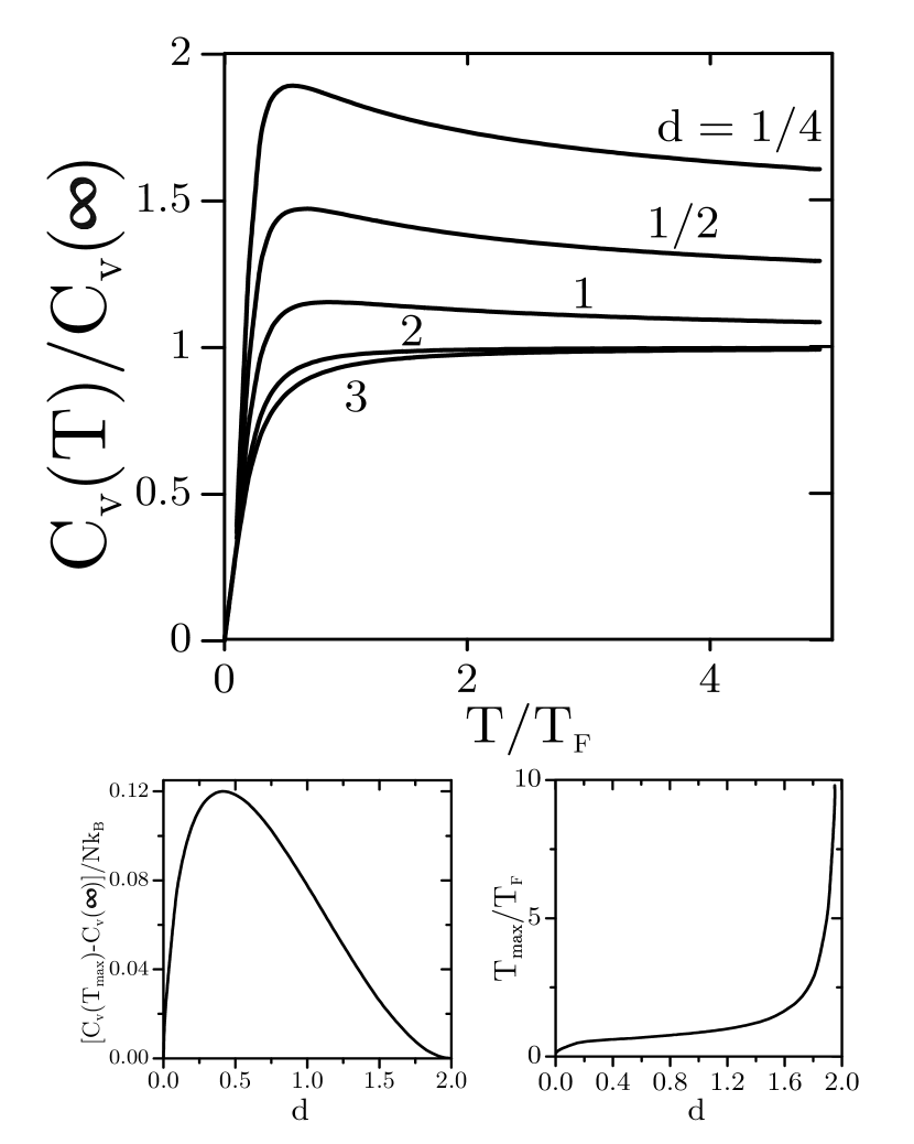
Figure 2: Specific heat for an IFG in $d=1/4,$ $1/2,$ $1,$ $2$ and $3$ dimensions. On the left bottom panel we show the maximum values of the specific heat as function of $d$ and on the right the values of the temperature $T_{\max}$ corresponding to the maxima in top panel.

Figure 3: The quantity $c_{T}^{2}(T)/c_{T}^{2}(0)$ where $c_{T}(T)$ is the isothermal sound velocity for an IFG as function of temperature $T/T_{F}.$ On the left bottom panel we show the minimum values in the isothermal sound velocity compared with $c_{T}(0)$ as function of Log $d$, and on the values of the temperature $T_{\min}$ corresponding to the minimum in top panel.

References

• [1] R. K. Pathria, Statistical Mechanics, 2nd Ed. (Pergamon, Oxford, 1996).
• [2] A.L. Fetter and J.D. Walecka, Quantum Theory of Many-Particle Systems (McGraw-Hill, NY, 1971).
• [3] E. Cetina, F. Magaña and A.A. Valladares, Am. J. Phys. 45, 960 (1977).
• [4] M.C. de Sousa Vieira and C. Tsallis, J. Stat. Phys. 48, 97 (1987).
• [5] B. DeMarco and D.S. Jin, Phys. Rev. A 58, R4267 (1998).
• [6] B. DeMarco and D.S. Jin, Science 285, 1703 (1999).
• [7] B. DeMarco, H. Rohner, and D.S. Jin, Rev. Sci. Instrum. 70, 1967 (1999)
• [8] M. Holland, B. DeMarco, and D.S. Jin, Phys. Rev. A 61, 053610 (2000).
• [9] R.M. Ziff, G.E. Uhlenbeck and M. Kac, Phys. Rep. 32, 169 (1977), p. 216.
• [10] V.C. Aguilera-Navarro, M. de Llano and M.A. Solís, Eur. J. Phys. 20, 177 (1999).
• [11] M. Casas, A. Rigo, M. de Llano, O. Rojo, and M.A. Solís, Phys. Lett. A 245, 55 (1998).
• [12] J.P. McKelvey, Solid State and Semiconductor Physics (Harper and Row, NY, 1966) p. 152.
• [13] N.W. Ashcroft and N.D. Mermin, Solid State Physics (Saunders College Publishing, San Diego, 1976) pp. 45 ff.
• [14] E. Corcoran and G. Zopette, Sci. Am., 25 (Sept. 1997).
• [15] E. Corcoran, Sci. Am., 122 (Nov. 1990).
• [16] C. Kittel and H. Kroemer, Thermal Physics, 2nd Ed. (W.H. Freeman and Company, New York, 1980).
Refer to caption