On the relationship between directed percolation and the synchronization transition in spatially extended systems

Abstract

We study the nature of the synchronization transition in spatially extended systems by discussing a simple stochastic model. An analytic argument is put forward showing that, in the limit of discontinuous processes, the transition belongs to the directed percolation (DP) universality class. The analysis is complemented by a detailed investigation of the dependence of the first passage time for the amplitude of the difference field on the adopted threshold. We find the existence of a critical threshold separating the regime controlled by linear mechanisms from that controlled by collective phenomena. As a result of this analysis, we conclude that the synchronization transition belongs to the DP class also in continuous models. The conclusions are supported by numerical checks on coupled map lattices too.

I Introduction

Synchronization in dynamical systems has recently become the subject of an intensive research activity for various reasons that range from the application to transmission of information, to the spontaenous onset of coherent behaviour and also because because it is one of the mechanisms controlling the degree of order present in a chaotic evolution. Most of the attention has been, so far, focused on the behaviour of low–dimensional systems. As a result of these investigations, several kinds of synchronizations have been identified (the most important being phase and complete synchronization) and the corresponding transition scenarios characterized PRK02 .

More recently, the interest has shifted towards high-dimensional chaos and, specifically, on the behaviour of extended systems, a context in which an overall picture is still lacking. In this paper, we devote our interest to complete synchronization in lattice systems. This kind of synchronization has been introduced and studied into two different setups. In the former one, identical copies of a given system (with different initial internal states) converge to the same trajectory, when forced with the same random signal. This, so-called stochastic, synchronization can occur only if the dynamics resulting from the stochastic forcing becomes linearly stable, i.e. the maximum Lyapunov exponent is negative FH92 ; MB94 ; P94 ; HF95 ; LZ98 . In the latter setup, two identical systems are coupled together: if the coupling strength is strong enough, both eventually follow the same, chaotic, trajectory. This is the so called chaotic synchronization. For it to be observed, it is sufficient that the transverse Lyapunov exponent is negative P92 . Therefore, in low–dimensional systems, synchronization transition can always be reduced to a linear stability problem.

On the other hand, recent numerical investigations BLT01 ; AP02 indicate that the synchronization scenario in spatially extended dynamical systems exhibits more complex and interesting features. In fact, the addition of the spatial structure may turn the linear stability problem of low–dimensional systems into a nonequilibrium phase-transition problem.

In analogy to low–dimensional systems, various coupling schemes have been already considered. For instance, “stochastic synchronization” has been studied in Coupled Map Lattices (CML’s), by adding the same spatio–temporal noise $\xi(x,t)$ to different trajectories, $u_{1}(x,t)$ and $u_{2}(x,t)$, of the same system BLT01 , according to the following scheme

$$u_{i}(x,t+1)=f[u_{i}(x,t)+\nabla_{\varepsilon}^{2}u_{i}(x,t)]+\sigma\xi(x,t)\quad,\quad i=1,2$$ (1)

where

$$\nabla^{2}_{\varepsilon}u(x,t)\equiv\frac{\varepsilon}{2}u(x+1,t)+\frac{\varepsilon}{2}u(x-1,t)-\varepsilon u(x,t)\quad,$$ (2)

is the short–hand notation for the discretized Laplacian operator ($\varepsilon$ plays the role of a diffusion constant) and $f[x]$ is a map of the unit interval able to generate chaotic behaviour. Moreover, $\sigma$ is the amplitude of the forcing term, $x$ is an integer index labeling the lattice sites, $t$ is a discrete time variable and the noise term is assumed to be bounded and $\delta$–correlated in space and time, i.e. $\langle\xi(x,t)\xi(y,s)\rangle\propto\delta_{x,y}\,\delta_{t,s}$. Synchronization is possible when the difference $w(x,t)=|u_{1}(x,t)-u_{2}(x,t)|$ between simultaneous configurations of the two systems converges everywhere to zero. The stability coefficient of the solution $w(x,t)=0$ is usually called the Transverse Lyapunov Exponent (TLE). In the context of stochastic synchronization, the evolution of a small $w(x,t)$ reduces to the tangent dynamics of the single CML, so that the TLE coincides with the maximum Lyapunov exponent of the noise-affected dynamics. Accordingly, synchronization can arise only when the stochastic forcing induces a negative maximum Lyapunov exponent. This is possible if the probability distribution of the state variable mostly concentrates in the region of the interval where the map acts as a contraction.

Alternatively, one can study the behavior of two directly coupled systems AP02

$$u_{1}(x,t+1) = (1-\sigma)f[u_{1}(x,t)+\nabla_{\varepsilon}^{2}u_{1}(x,t)]+\sigma f[u_{2}(x,t)+\nabla_{\varepsilon}^{2}u_{2}(x,t)],$$

$$u_{2}(x,t+1) = (1-\sigma)f[u_{2}(x,t)+\nabla_{\varepsilon}^{2}u_{2}(x,t)]+\sigma f[u_{1}(x,t)+\nabla_{\varepsilon}^{2}u_{1}(x,t)]\quad.$$ (3)

At variance with the previous case, the coupling strength $\sigma$ modifies the evolution law of $w(x,t)$, by adding a stabilizing term, while it leaves unaffected the dynamics of the fully synchronized regime. Accordingly, the TLE may become negative, while the maximum Lyapunov exponent, unchanged, remains positive.

While the negativity of the TLE is always a necessary condition to observe synchronization in spatially extended systems, for smooth enough dynamical systems, it proves to be sufficient too. In fact, the study of stochastic and chaotic synchronization, carried on in Refs. BLT01 and AP02 , respectively, have shown that synchronization occurs as soon as the TLE becomes negative and, correspondingly, the propagation velocity of finite-amplitude perturbation vanishes. In particular, Ahlers and Pikovsky AP02 argue that the dynamics of the coarse-grained absolute value $\tilde{w}$ of the difference field is described by the following stochastic partial differential equation,

$$\partial_{t}\tilde{w}(x,t)=D\nabla^{2}\tilde{w}(x,t)+c_{1}\tilde{w}(x,t)-c_{3}\tilde{w}^{3}(x,t)+\tilde{w}(x,t)\eta(x,t)\quad,$$ (4)

where $D>0$, $c_{3}>0$ and the Gaussian noise term $\eta$ is $\delta$–correlated in space and time, i.e. $\langle\eta(x,t)\eta(y,s)\rangle\propto\delta(x-y)\delta(t-s)\,$. This equation is formally equivalent to the mean–field equation of the class of Multiplicative Noise (MN) nonequilibrium critical phenomena GMT96 . By a Hopf–Cole transformation, $h(x,t)=-\ln\tilde{w}(x,t)$, the above equation can be transformed into foot1

$$\partial_{t}h(x,t)=D\nabla^{2}h(x,t)-D(\nabla h(x,t))^{2}-(c_{1}-\frac{1}{2})+c_{3}e^{-2h(x,t)}+\eta(x,t)$$ (5)

describing the critical behaviour associated with the depinning transition of a Kardar–Parisi–Zhang (KPZ) interface from a hard substrate. Numerical analysis confirms that the critical exponents evaluated for the two different coupling schemes are both compatible with those predicted for the MN model.

On the other hand, it has been observed that in the presence of strong and localized nonlinearities, the non-synchronized regime may coexist with a negative TLE BLT01 ; AP02 . In this case, the transition does occur when the propagation velocity of finite–amplitude perturbations vanishes, while its critical properties turn out to belong to the class of Directed Percolation. Such an equivalence has been found by noticing that the fraction of non-synchronized sites (defined as those points where $|w(x)|$ is larger than some small fixed threshold) is the appropriate order parameter corresponding to the fraction of active sites in DP.

In this case, one cannot follow the same derivation as above, because even close to the critical point, the evolution equation for $w(x,t)$ cannot be linearized, since it is precisely the nonlinear effects which guarantee a propagation of finite–amplitude perturbations in the presence of a negative TLE. It is worth recalling that in the formulation of Reggeon Field Theory, the DP transition is described by the effective equationMD99 ; G95 ; H00

$$\partial_{t}\rho(x,t)=D\nabla^{2}\rho(x,t)+c_{1}\rho(x,t)-c_{2}\rho^{2}(x,t)+\sqrt{\rho(x,t)}\eta(x,t)\quad,$$ (6)

where $\rho(x,t)$ is the density of active sites and $c_{2}>0$. Behind the similarity between this and Eq. (4), one should notice the crucial difference in the noise amplitude: the square-root versus linear dependence on $\rho$ is indeed responsible for turning the MN critical behaviour into a DP-like one. In this paper, we plan to explain why the presence of a discontinuity (or a strong nonlinearity) may lead to the effective equation (6). To this aim, in Section 2 we introduce a simple Random Multiplier (RM) model as an effective equation for the time evolution of the difference variable $w(x,t)$ for discontinuous and strongly nonlinear CML’s. This model was originally introduced in GLP02 to account for the mechanism of propagation of information in stable chaotic systems. We analyze its phase diagram, and we also discuss how the synchronization transition may be modified when a true discontinuity in the dynamics is changed into a strongly nonlinear continuous mapping. The relation between the RM model and the DP mean–field equation (6) is analyzed in Section 3.

There is a further basic question that will be addressed here. All microscopic models that are known to exhibit a DP critical behaviour are defined by referring to discrete and finite state variables, such as the probabilistic cellular automaton model proposed by Domany and Kinzel DK84 . In such cases, the so–called “absorbing state” can be unambiguously identified. For instance, in the cellular automaton of Ref. DK84 , a sequence of “$0$”s can only change from its boundaries (this is the reason they are defined as contact processes). In the context of synchronization, the dynamical variable is continuous and the condition $w(x,t)=0$ is never exactly fulfilled at any finite time, even in a system of finite size. As a consequence, in numerical experiments BLT01 ; AP02 one has to fix a small, but somehow arbitrary, threshold value, below which the trajectories are assumed to be synchronized. The same numerical simulations show that, independently of the dynamical rule, when the space average of $w(x,t)$ decreases below a threshold value ${\mathcal{O}}(10^{-5})$ it does not grow again. However, one cannot a priori exclude that a large fluctuation of some local multiplier drives the system out of this weakly absorbing state. On the contrary, it looks plausible to assume that in an infinite system such a large fluctuation occurs with probability one. In Section 4 we tackle the problem of the existence of an effective absorbing state even in the presence of a continuous state variable. The study of the first passage time required for the space average of the difference variable $w(x,t)$ to go through a series of decreasing thresholds clarifies that, contrary to intuition, it is possible to assign an effective finite “measure” to the synchronized, i.e. absorbing, state. Finally, conclusions are drawn in Section 5.

II The Random Multiplier Model: definition and phase diagram

In this section, we introduce the RM model with the aim of closely reproducing the synchronization transition occurring in coupled piecewise linear maps of the type,

$$f(x)=\left\{\begin{array}[]{lr}x/\alpha_{1}&0\leq x<\alpha_{1}\\ 1-(x-\alpha_{1})/\alpha_{2}&\alpha_{1}\leq x<\alpha_{1}+\alpha_{2}\\ (x-\alpha_{1}-\alpha_{2})/\alpha_{1}&\alpha_{1}+\alpha_{2}\leq x\leq 1\end{array}\right.\quad,$$ (10)

where $0<\alpha_{1}<1$ and $0<\alpha_{2}<1-\alpha_{1}$. For any $\alpha_{2}>0$, the map is continuous with a highly expanding middle branch (when $\alpha_{2}\ll 1$). In the limit $\alpha_{2}=0$, $f(x)$ reduces to the discontinuous Bernoulli map with expansion factor $1/\alpha_{1}$.

In the bidirectional synchronization setup (3), the corresponding TLE is AP02

$$\lambda_{\perp}=\lambda_{M}+\ln(1-2\sigma).$$ (11)

where $\lambda_{M}$ is the maximum Lyapunov exponent of the single, uncoupled, chain. Therefore, linear stability analysis indicates that a small deviation $w(x,t)=|u_{1}(x,t)-u_{2}(x,t)|$ is contracted when $\sigma>(1-1/\lambda_{M})/2$. However, this is not the whole story even in the absence of multiplier fluctuations, because whenever $u_{1}(x,t)$ and $u_{2}(x,t)$ fall on different sides of the map-discontinuity, $w(x,t)$ becomes at once of order 1, being amplified by a factor close to $1/w(x,t)$. The probability of such events depends on the probability density of the variables $u_{i}$: in the case of a sufficiently smooth distribution across the discontinuity, the probability is, to a leading order, proportional to $w$ itself foot2 . The same qualitative behaviour does occur also for $\alpha_{2}>0$, except that now, when $w<\alpha_{2}$, the amplification factor cannot be larger than $(1-2\sigma)\alpha_{2}$. Moreover, the probability of such amplifications does no longer depend on $w$.

In the following, instead of determining the local dynamics of $w$ from the actual evolution of $u_{1}(x,t)$ and $u_{2}(x,t)$, we prefer to write a self-contained equation, where the occasional amplifications follow from a purely stochastic dynamics that simulates the CML. More precisely, we introduce the model

$$v(x,t)=(1+\nabla^{2}_{\varepsilon})w(x,t)\quad,$$ (12)

with

$$\begin{array}[]{llr}w(x,t+1)=\left\{\begin{array}[]{ll}1,&\mbox{w.p.}\quad p=av(x,t)\\ av(x,t),&\mbox{w.p.}\quad 1-p\end{array}\right.,\quad\mbox{if $v(x,t)>\Delta$,}\\ \\ w(x,t+1)=\left\{\begin{array}[]{ll}v(x,t)/\Delta,&\mbox{w.p.}\quad p=a\Delta\\ av(x,t),&\mbox{w.p.}\quad 1-p\end{array}\right.,\quad\mbox{if $v(x,t)\leq\Delta$,}\end{array}$$ (20)

where $a$ and $\Delta$ replace $(1-2\sigma)/\alpha_{1}$ and $\alpha_{2}/(1-2\sigma)$, while w.p. is a shorthand notation for “with probability”. Only positive multipliers are assumed in order to guarantee a positive defined $w(x,t)$ (simulations do confirm that the sign does not play a relevant role). Finally, periodic boundary conditions are assumed on a lattice of size $L$.

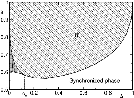
Figure 1: Phase diagram of the RM model. In the two shaded regions ( $I$ and $II$) the synchronized phase is unstable; in fact, above the solid line $v_{F}>0$. Along the dashed line, the TLE changes sign, so that region $I$ corresponds to the linearly stable, but nonlinearly unstable regime, while $II$ corresponds the linearly unstable region. Above $\Delta=\Delta_{c}$, the TLE vanishes together with $v_{F}$.

The advantage of playing with this model is that it explicitly avoids the possibly subtle correlation that may be generated during the deterministic evolution of the CML and thereby spoiling the asymptotic behaviour of the observables we are interested in. Besides the probabilistic, rather than deterministic, choice of the amplification factor, the only other difference between the stochastic model (20) and the original set of two coupled CMLs is the distribution of the amplification factors that is dichotomic in the former case. We see no reason why this difference should affect the transition scenario.

Moreover, in order to maximize propagation effects (that are responsible for the propagation of finite-size perturbations) we shall restrict to the case $\varepsilon=2/3$ (the so called “democratic” coupling). Some rough numerical analyses do not, indeed, reveal qualitative changes when $\varepsilon$ is varied around $2/3$.

The most general way of testing the stability of the synchronized phase is by monitoring the evolution of a droplet of the unsynchronized phase. By denoting with $N(t)$ the droplet size, i.e. the number of unsynchronized sites, at time $t$, the propagation velocity can be defined as

$$v_{F}\equiv\lim_{t\rightarrow\infty}\frac{N(t)-N(0)}{2t}\quad.$$ (21)

A negative TLE (the maximum Lyapunov exponent of model (20)) implies that any infinitesimal perturbation does decay. In spite of this linear stability, in Ref. GLP02 it has been shown that $v_{F}$ can be positive, implying that the unsynchronized phase sustains itself and invades the synchronized one. By performing detailed simulations for different values of the parameters $a$ and $\Delta$, we have been able to construct the phase diagram plotted in Fig. 1. The solid line, along which $v_{F}=0$, separates the synchronized from the unsynchronized phase (shaded region). The dashed line, along which the TLE is equal to 0, splits the unsynchronized phase into a linearly stable ($I$) and unstable ($II$) region. In the former one (ending approximately at $\Delta=\Delta_{c}\approx 0.15$), the nonlinear amplification mechanism prevails over the linear contraction induced by the negative TLE. Above $\Delta_{c}$, the TLE changes sign exactly where $v_{F}$ vanishes too.

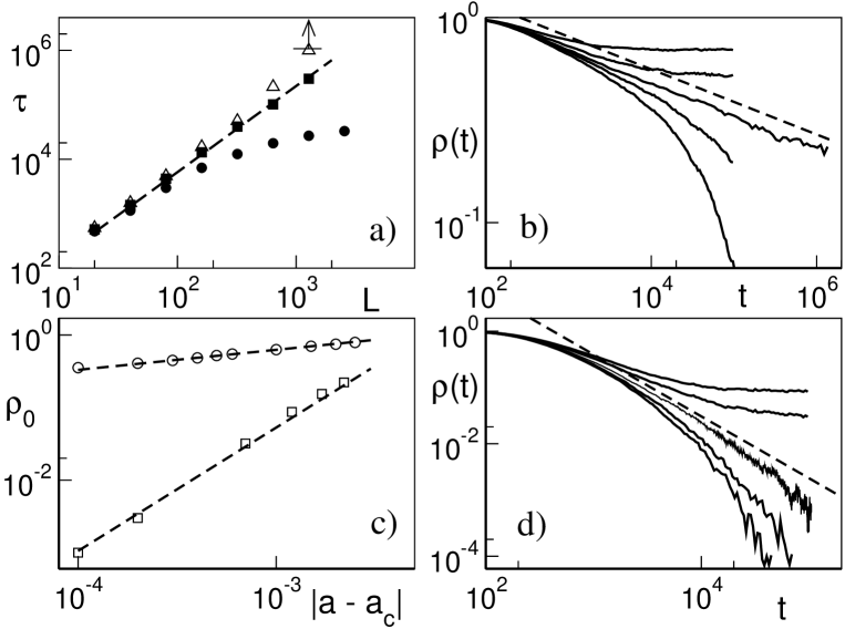
Figure 2: Power law scaling behaviour in the RM model. In all graphs, the dashed lines correspond to the expected scaling behaviour (DP in a), b) and c); MN in d)). a) Absorption time as a function of system size for $\Delta=0$. Triangles corresponds to $a=0.6070$, squares to $a=0.6063$ and circles to $a=0.6051$. b) Density of unsynchronized sites as a function of time for $\Delta=0.1$. The five solid lines correspond to (from top to bottom) $a=0.591$, $a=0.59$, $a=0.58955$, $a=0.5893$ and $a=0.5890$, respectively. c) Asymptotic density of unsynchronized sites as a function of the distance from criticality. Circles corresponds to $\Delta=0.1$ and squares to $\Delta=0.2$. d) Density of unsynchronized sites as a function of time for $\Delta=0.2$. The five solid lines correspond to (from top to bottom) $a=0.568$, $a=0.5675$, $a=0.5668$, $a=0.5664$ and $a=0.5662$. All the graphs are plotted in a doubly logarithmic scales.

Numerical analysis of stochastic synchronization in CML BLT01 suggests that when the TLE vanishes together with $v_{F}$, the critical properties of the synchronization transition are those of the MN class, while the transition is DP-like whenever $v_{F}$ only vanishes (the TLE remaining negative).

Before entering a quantitative discussion about the nature of the transition in the present model, it is worth noticing a difference between the regimes $I$ and $II$. Linear instability in $II$ ensures that any finite perturbation of a synchronized state remains finite forever independently of the chain length. On the other hand, in $I$, a finite perturbation eventually dies in a finite chain. The reason why the synchronized regime can nevertheless be considered unstable is that the average life time of the perturbation diverges exponentially with the chain length. This is a typical property of systems in DP universality class and it can be traced back to the peculiar nature of the “square root” noise amplitude in Eq. (6) M98 .

A preliminary numerical analysis of the critical properties of the RM model for $\Delta=0$ and $\Delta=0.01$ has been already published in GLP02 . Here we both perform more accurate simulations and extend the previous study to larger values ($\Delta=0.1$, 0.2) in order to find a signature of the change of critical behavior. In all cases, $a$ is chosen to be the control parameter, while the averaged (over different noise realizations) density $\rho(t)$ of unsynchronized sites will be the order parameter. The definition of $\rho$ requires to fix a small threshold $W$ to discriminate between synchronized ($w(x,t)<W$) and unsynchronized ($w(x,t)>W$) sites. In principle, $\rho(t)$ depends on $W$, both because the perturbation reaches different thresholds at different times and resurgencies can occur. Numerical analysis, however, indicates that, in practice, if $W$ is chosen on the order or smaller than $10^{-5}$ no appreciable differences are observed. We shall come back to this problem in Sec. 4, to provide a more sound justification for the adopted procedure.

In order to test the relationship between synchronization transition and the DP critical phenomenon, we have investigated the scaling behaviour in the vicinity of the transition. In DP it is known that, at criticality, the dependence of the density $\rho(t)$ on $t$ and $L$ is described by the scaling relation H00

$$\rho(t)=L^{-\delta z}g\left(\frac{t}{L^{z}}\right)\quad,$$ (22)

where $z$ is the so-called dynamical exponent accounting for the dependence of the average time $\tau$ needed for $\rho$ to vanish with the system size $L$ ND88 ,

$$\tau\sim L^{z}\quad\quad\quad a=a_{c}\quad.$$ (23)

Since for small $\theta=t/L^{z}$, the scaling function behaves as $g(\theta)\sim\theta^{-\delta}$, the exponent $\delta$ turns out to describe the power-law decay of $\rho(t)$

$$\rho(t)\sim t^{-\delta}\quad\quad\quad a=a_{c}\quad.$$ (24)

Finally, the exponent $\beta$ characterizes the scaling behaviour of the saturated density of active sites $\rho_{0}(t)$ as a function of the distance from the critical value,

$$\rho_{0}\sim(a-a_{c})^{\beta}\quad\quad\quad a>a_{c}\quad.$$ (25)

In analogy with usual nonequilibrium phase transitions, $z$, $\delta$, and $\beta$ are expected to characterize all critical properties of the synchronization transition as well. In fact, simple dimensional arguments show that the exponents ruling the power law divergence exhibited by space- and time-correlation functions (while approaching the critical point) are linked to the previous ones by the standard relations

$$\nu_{\parallel}=\frac{\beta}{\delta}\quad,\quad\quad\nu_{\perp}=\frac{\nu_{\parallel}}{z}\quad.$$ (26)

Some of the scaling behaviors have been plotted in Fig. 2 to show the quality of the results, while a complete summary of the exponents are reported in Table 1, together with the best known estimates for the DP J96 and the MN TGM97 class.

The dynamical exponent has been estimated by averaging the behaviour of relatively small systems (from $L=2^{5}$ to $L=2^{10}$) over a large number of noise realizations (of order $10^{3}$). In order to minimize finite-size effects, the exponents $\delta$ and $\beta$ have been estimated from the time evolution of a single system of size $L=2^{20}$, relying on the large size to reduce statistical fluctuations. In the MN context we have not been able to estimate $z$ through the measure of the average synchronization time, but we verified, through finite size-scaling (22), that the value of the dynamical exponent is compatible with the theoretical prediction.

Interestingly, similar results are obtained by adopting a different order parameter, i.e. the space averaged difference variable $w(t)=\langle w(x,t)\rangle_{x}$. Also in this case, both $\langle w(t)\rangle$ (where $\langle\cdot\rangle$ denotes ensemble average) and the absorption time $\tau_{1}$, defined as the average time required for $w(t)$ to become smaller than some threshold $W$, are found to follow the same critical scaling laws. The application of coarse-graining suggests that the space average is the “natural” order parameter in the context of both equilibrium and nonequilibrium critical transitions.

	$\Delta=0$	$\Delta=0.01$	$\Delta=0.1$	$\Delta=0.2$	DP	MN
$z$	$1.56\pm 0.06$	$1.58\pm 0.02$	$1.54\pm 0.06$	$1.5$ *	$1.580745\pm 10^{-6}$	$1.53\pm 0.07$
$\delta$	$0.155\pm 0.005$	$0.15\pm 0.01$	$0.159\pm 0.002$	$1.2\pm 0.1$	$0.159464\pm 6\cdot 10^{-6}$	$1.10\pm 0.05$
$\beta$	$0.24\pm 0.02$	$0.27\pm 0.01$	$0.27\pm 0.01$	$1.8\pm 0.1$	$0.276486\pm 6\cdot 10^{-6}$	$1.70\pm 0.05$
$a_{c}$	$0.6063\ldots$	$0.605\ldots$	$0.5895\ldots$	$0.5668\ldots$

Table 1: Numerical results concerning the $z$ the $\delta$ and the $\beta$ exponent of the RM model are compared with the best available estimates. Values for $a_{c}$ indicate our best estimates of the critical point. Errors have been estimated as the maximum deviation from linearity in the log-log plot that it is used to extract the scaling law. * Indicates a value compatible with the theoretically predicted one, $z=1.5$ (see text).

III From the RM model to the DP field equation

In this section we investigate the connection between the RM model and the DP field equation (6). Let us first consider the simple case $\Delta=0$ that corresponds to a discontinuous but otherwise uniformly contracting local map. Eq. (20) can be recasted as

$$w(x,t+1)=2av(x,t)-a^{2}v^{2}(x,t)+g(v)\xi^{\prime}(x,t)\quad,$$ (27)

where $\xi^{\prime}(x,t)$ is a zero-average $\delta$-correlated noise with unit variance. In fact,

$$\xi^{\prime}(x,t)=\frac{1}{g(v)}[\xi_{v}(x,t)-\langle\xi_{v}\rangle]\quad,$$ (28)

where

$$\xi_{v}(x,t)=\left\{\begin{array}[]{ll}1-v(x,t),&\mbox{w.p.}\quad p=av(x,t)\\ (a-1)v(x,t),&\mbox{w.p.}\quad 1-p,\end{array}\right.\quad,$$ (29)

and

$$\langle\xi_{v}\rangle = (2a-1)v-a^{2}v^{2}$$ (30)

$$g^{2}(v) = \langle\xi_{v}^{2}\rangle-\langle\xi_{v}\rangle^{2}=a-3a^{2}v^{2}+3a^{3}v^{3}-5a^{4}v^{4}\quad.$$ (31)

If we now introduce the coarse grained variable $\rho(x,t)=\overline{w(x,t)}$ (where the bar denotes an average over a suitable space-time cell), we have that $\overline{v(x,t)}=\rho(x,t)+\frac{\varepsilon}{2}\nabla^{2}\rho(x,t)$ so that Eq. (27) yields,

$$\begin{array}[]{ll}\partial_{t}\rho(x,t)=&a\varepsilon\nabla^{2}\rho(x,t)+(2a-1)\rho(x,t)-a^{2}\rho^{2}(x,t)+a^{2}\varepsilon\rho(x,t)\nabla^{2}\rho(x,t)+\\ &\frac{(a\varepsilon)^{2}}{4}\left[\nabla^{2}\rho(x,t)\right]^{2}+g\left(\rho(x,t)+\frac{\varepsilon}{2}\nabla^{2}\rho(x,t)\right)\eta(x,t)\quad.\end{array}$$ (32)

where, according to the central limit theorem KTH85 , the coarse grained noise term $\eta(x,t)$ is Gaussian and $\delta$-correlated in time and space. According to standard renormalization-group arguments, H00 ; MD99 ; G95 the terms of order $(\nabla^{2}\rho)^{2}$ and $\rho\nabla^{2}\rho$ can be shown to be irrelevant, as well as the terms of order higher than or equal to $\rho$ and $\sqrt{\nabla^{2}\rho}$ appearing in the noise amplitude $g(\rho+\frac{\varepsilon}{2}\nabla^{2}\rho)$.

From the definition (31) of $g$ and after discarding the irrelevant terms, the above equation reduces to

$$\partial_{t}\rho(x,t)=a\varepsilon\nabla^{2}\rho(x,t)+(2a-1)\rho(x,t)-a^{2}\rho^{2}(x,t)+\sqrt{a\rho(x,t)}\eta(x,t).$$ (33)

which is nothing but Eq. (6), thus proving that the synchronization transition in discontinuous CML’s can be traced back to a DP nonequilibrium phase transition.

Let us now turn our attention to the more general case $\Delta>0$, which corresponds to a continuous local mapping. According to Eq. (20), we have now to deal with two different kinds of noise, depending whether $v(x,t)>\Delta$ or $v(x,t)\leq\Delta$. By repeating the same formal derivation as in the previous case, we find that Eq. (33) still holds when $\rho>\Delta$, while for $\rho(x,t)<\Delta$ it must be replaced by the equation

$$\partial_{t}\rho(x,t)=\frac{a\varepsilon}{2}\left(2-a\Delta\right)\nabla^{2}\rho(x,t)+(2a-1-a^{2}\Delta)\rho(x,t)+h(w)\eta(x,t)\quad,$$ (34)

where

$$h(w)=\rho(x,t)\sqrt{\frac{a}{\Delta}-3a^{2}+(2+5\Delta)a^{3}-(3+2\Delta)\Delta a^{4}+(1-\Delta^{2})\Delta a^{5}}\quad.$$ (35)

Accordingly, in Eq. (34), the noise amplitude is proportional to the field itself, so that one should be led to the naive conclusion that the DP critical behaviour is destroyed as soon as $\Delta$ is finite, or, equivalently, that any CML system characterized by a continuous local mapping cannot exhibit a DP-like synchronization transition. However, the simulations described in the previous section suggest that DP-like transition can still been found for small but finite values of $\Delta$. In the next sections we shall present theoretical arguments supporting such numerical findings.

IV First passage times

In this section we clarify the problem of how and when it is possible to observe a DP-like scenario in models like the RM one, with no clearly identifiable absorbing state. As already noted in GLP02 , in any finite system (of length $L$) there always exists a finite probability for a generic configuration to be contracted forever, i.e. absorbed. A lower bound to such a probability is (in the discontinuous case),

$$P=\left[\prod_{n=1}^{\infty}(1-w_{M}a^{n})\right]^{L}\quad,$$ (36)

where

$$w_{M}=\max_{x}{w(x,0)}\quad.$$ (37)

However, since the null state, $w(x,t)=0$, is reached in an infinite time, this configuration cannot be attained with perfect accuracy in numerical simulations and one is, in fact, obliged to fix a small but finite threshold.

The best way we have found to characterize the dependence of the perturbation evolution on its size is through an indicator closely related to the finite-size Lyapunov exponent (FSLE) introduced in Ref. ABCPV96 . With reference to a perturbation initially set equal to 1 ($w(x,0)=1,\quad x=1\ldots L$), we introduce the first passage time $\tau_{q}(W)$, defined as the (ensemble) average time required by the $q$-th norm of the state vector ${\bf w}(t)$,

$$||{\bf w}(t)||_{q}=\left[\frac{1}{L}\sum_{i=1}^{L}w_{i}^{q}(t)\right]^{\frac{1}{q}}$$ (38)

to become smaller than some threshold $W$ for the first time. At variance with Ref. ABCPV96 ; CT01 , we do not care if the evolution of the perturbation is non monotonous: as we shall see, in this context, the analysis does not only remain meaningful, but even more, it allows identifying the reason for the existence of a DP-like scenario even in the context of the continuous model.

At variance with the standard Lyapunov exponent, the FSLE does depend on the choice of the norm (in particular, on the $q$-value in Eq. (38)). This circumstance is often considered as a difficulty, hindering a proper definition of FSLE: we prefer to see it as an indication of a richer class of phenomena associated with the evolution of finite-amplitude perturbations. Anyway, it has been noticed in Sec. II that the “natural” order parameter of DP transition is the spatial average of the state vector. Accordingly, we have decided, in the present context, to fix $q=1$ (that corresponds to performing an arithmetic average) and to drop, for the sake of simplicity, the dependence on $q$.

The FSLE $\Lambda(W)$ can be introduced by first fixing a sequence of decreasing thresholds $W_{n}$, $n=0,1,2,\ldots$,

$$\frac{W_{n}}{W_{n-1}}=r\quad,\quad\quad r<1\quad,$$ (39)

and by then defining

$$\Lambda(W_{n})=\frac{\ln r}{\tau(W_{n+1})-\tau(W_{n})}\quad,$$ (40)

where the dependence on the “discretization” $\ln r$ is left implicit. In the limit $r\to 1$, the definition becomes

$$\Lambda(W)=\left[\frac{d\,\tau(W)}{d\,(\ln W)}\right]^{-1}\quad.$$ (41)

In the further limit $W\to 0$, $\Lambda(W)$ reduces to the usual Lyapunov exponent $\lambda$, independently of the adopted $q$-value. When $\Delta=0$, $\lambda=\ln a$.

IV.1 Uncoupled limit

In the uncoupled limit, $\varepsilon=0$, each site converges independently to the synchronized state (as long as $a<1$). In spite of the low-dimensionality of the problem, even in this case, an analytic expression for the FSLE can be obtained only at the expense of introducing further approximations. We shall see that the resulting expression can be nevertheless profitably used even in the coupled regime.

By setting $r=a$ and restricting ourselves to the case $\Delta=0$, it easy to show (see appendix A) that

$$\tau(W_{n})=\frac{\tau(W_{n-1})+1}{1-W_{n}}\quad,$$ (42)

where $\tau(W_{0})=0$, $W_{n}=a^{n}$. By inserting Eq. (42) in Eq. (40) one obtains

$$\Lambda(W_{n})=\frac{1-a\,W_{n}}{1+a\,W_{n}\,\tau(W_{n})}\ln a\quad.$$ (43)

Eq. (42) implies that, for $n\to\infty$,

$$\tau(W_{n})\sim n+n_{0}=\frac{\ln W_{n}}{\ln a}+n_{0}\quad.$$ (44)

By inserting Eq. (44) into Eq. (43) and recalling that $\lambda=\ln a$ (for $\Delta=0$), we obtain

$$\Lambda(W_{n})=\frac{1-a\,W_{n}}{1+an_{0}W_{n}+(a/\lambda)W_{n}\ln W_{n}}\lambda\quad.$$ (45)

As we are interested in describing the region where $W_{n}\ll 1$, and owing to relative smallness of $a$ ($a\ll n_{0}$), this equation can be further simplified to

$$\Lambda(W)=\frac{\lambda}{1+b_{0}W-b_{1}W\ln W}\quad,$$ (46)

where we have also dropped the unnecessary dependence on the index $n$. In the $W\to 0$ limit, the leading correction to the standard Lyapunov exponent is provided by the term proportional to $b_{1}$. From the structure of Eq. (46), it is natural to interpret the inverse of $b_{1}$ as the critical threshold $W_{c}$, below which the dynamics of the uncoupled system is dominated by the maximum Lyapunov exponent $\lambda$.

From Eq. (46) and by integrating Eq. (41), it is possible to derive also an analytic expression for the first passage time $\tau(W)$,

$$\tau(W)=\int\Lambda(W)^{-1}d\,(\ln W)\approx\frac{1}{\lambda}\left[\ln W+(b_{0}+b_{1})W-b_{1}W\ln W\right]+b_{2}\quad,$$ (47)

where $b_{2}$ is the integration constant. In principle, one could imagine of determining $b_{2}$ by imposing $\tau(1)\equiv b_{2}-b_{1}/\lambda$ equal to 0, since the evolution starts precisely from $W=1$. However, we cannot expect our perturbative formula to describe correctly the initial part of the contraction process. Therefore, $b_{2}$ must be determined independently.

IV.2 General case and scaling arguments

In the coupled case, we have not been able to derive an analytical expression for the FSLE. Nevertheless, a comparison with the numerical results has revealed that Eqs. (46,47) describe in a reasonable way the dependence of $\Lambda$ and $\tau$ on $W$ even in the continuous model. However, while $\lambda$ still denotes the standard Lyapunov exponent of the process and can thus be computed independently, now $b_{0}$, $b_{1}$, and $b_{2}$ have to be determined by fitting the numerical data. We have preferred to keep also the term proportional to $b_{0}$ (relevant only for relatively large $W$-values), since its presence guarantees a much better reproduction of the numerical data. In Fig. 3a, we see that Eq. (47) provides a good parametrization of the numerically determined $\tau$-values over a wide range of thresholds, both in the discontinuous and the continuous model (see the solid curves). In panel b) we notice that, although the theoretical expression (46) does not provide an equally good description of the FSLE, it is nevertheless able to pinpoint the crossover towards the small-amplitude behaviour of the perturbation. We will see that the possibility of identifing the largest scale (defined by $1/b_{1}$) over which the linearized dynamics (described by the standard Lyapunov exponent) sets in represents a crucial point of our analysis.

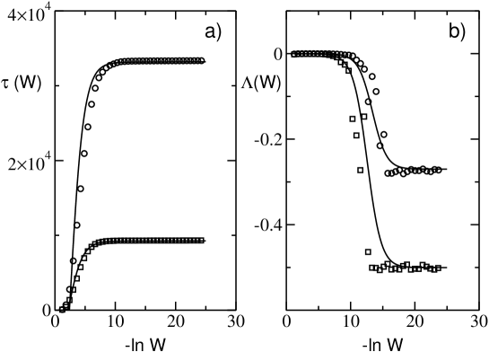
Figure 3: Numerical data for the first passage time (left panel) and the FSLE (right panel) at the critical point are fitted with Eq. (47) and Eq. (41) (full lines). Circles refers to $\Delta=0.01$, $L=256$, $a_{c}=0.6055$ and squares to $\Delta=0$, $L=128$, $a_{c}=0.6063$.

It is now natural to ask to what extent Eq. (47) is able to account for the scaling behaviour in the vicinity of the transition. By replacing $\rho$ with $W$ in Eq. (22) and $t$ with the first passage time $\tau$, one expects that, at criticality,

$$W=L^{-\delta z}g(t/L^{z})\quad.$$ (48)

Inversion of this equation leads to

$$\tau(W)=L^{z}g^{-1}(WL^{\delta z})\quad.$$ (49)

Before mutually comparing the two expressions (47,49), it should be first stressed that they have been introduced to address different questions. On the one hand, Eq. (47) is an approximate expression introduced to account for the crossover towards the $W$-range where the dynamics is controlled by linear mechanisms and no scaling behavioiur should be expected. On the other hand, Eq. (49) is a rigorous but implicit statement about the scaling region only.

Compatibility between Eqs. (47) and (49) requires a proper dependence of $b_{0}$, $b_{1}$ and $b_{2}$ on the systems size $L$, namely

$$b_{0} = -\lambda\left[\tilde{b}_{0}-\tilde{b}_{1}(1+\delta z\ln L)\right]L^{z(1+\delta)}$$ (50)

$$b_{1} = -\lambda\tilde{b}_{1}L^{z(1+\delta)}$$ (51)

$$b_{2} = \tilde{b}_{2}L^{z}\quad,$$ (52)

where $\tilde{b}_{0}$, $\tilde{b}_{1}$, and $\tilde{b}_{2}$ are suitable positive constants. By inserting Eq. (52) into Eq. (47), one finds that

$$\tau(W)=\frac{\ln W}{\lambda}-L^{z}\left[\tilde{b}_{0}WL^{z\delta}-\tilde{b}_{1}WL^{z\delta}\ln(WL^{\delta z})+\tilde{b}_{2}\right]\quad,$$ (53)

from which we see that the first term in the r.h.s. is the only one which does not follow the required scaling law (49). In fact, $(\ln W)/\lambda$, accounts for the linearly stable behaviour in a regime where a finite-state model (such as, e.g., the famous Domany-Kinzel model DK84 ) would be otherwise characterized by a perfect absorption (when a configuration of all 0’s is attained).

In order to test the correctness of the whole picture, we have studied the dependence of $b_{1}$ and $b_{2}$ on $L$. In Fig. 4, their behaviour is plotted at criticality for the discontinuous and the continuous model: both quantities show a good agreement with the power law divergence predicted by Eq. (52) ($z\approx 1.58$ and $z(1+\delta)\approx 1.82$). As for the last parameter $b_{0}$, given its involved dependence on $L$ and the approximate character of Eq. (53), we can only claim that its dependence is qualitatively consistent with the theoretical prediction.

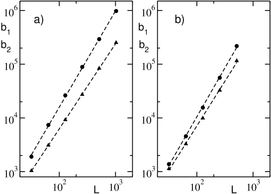
Figure 4: Finite-size scaling behaviour at the critical point of both $b_{1}$ and $b_{2}$ for $\Delta=0$ and $a_{c}=0.6063$ (left panel) and $\Delta=0.01$ and $a_{c}=0.6055$ (right panel). The dashed lines indicate the best power law fit. Left: $b_{1}$ (circles) scales as $L^{1.79}$, while $b_{2}$ (triangles) scales as $L^{1.58}$. Right: $b_{1}$ (squares) scales as $L^{1.82}$, while $b_{2}$ (diamonds) scales as $L^{1.66}$.

One of the most important results of our study is the objective identification of a threshold $W_{c}=1/|b_{1}|$, below which linear stability analysis holds and its scaling dependence on $L$ ($W_{c}\sim L^{-z}$). In a model like the cellular automaton considered by Domany and Kinzel DK84 , absorption in a finite system occurs when all sites collapse onto the absorbing state: this means that the minimal meaningful density that can be considered is $\rho_{m}=1/L$. In the present context, $W_{c}$ plays the role of $\rho_{m}$: below $W_{c}$, the critical behaviour is dominated by the linearly stable dynamics. The difference between the two systems lies in the scaling dependence of the maximal resolution on $L$. Since $W_{c}$ decreases faster than $1/L$ this means that, e.g., the scaling range for $W_{c}$ is wider in the present model than in finite-state systems.

Finally, we comment about the reason why the range of validity of the linear stability analysis can eventually vanish even in models like the continuous RM, where every perturbation locally smaller than $\Delta$ should behave linearly. The reason is that $\tau(W)$ is defined as the average first-passage time: even if the perturbation is homogeneously small, if $L$ is sufficiently large, some occasional amplification may occur and drive, on the average, the system out of the linear region. It is only below $W_{c}$ that such sporadic resurgencies are sufficiently rare not to modify significantly the stable linear behaviour.

V Conclusions and open problems

In this paper we have expounded a partially rigorous argument to show why the synchronization transition in spatially extended systems may belong to the DP universality class. Although our theoretical considerations restrict to the discontinuous RM model, scaling analysis of the first-passage time $\tau(W)$ suggests that the transition belongs to the DP class also in a finite parameter region of the continuous model. Since direct numerical simulations in the more physical class of CMLs have been basically restricted to discontinuous maps, we find it wise to test the validity of our conclusions also in the context of continuous, though highly-nonlinear maps. Accordingly, we have considered two lattices of maps coupled as in Eq. (3); the local map is chosen similar to those defined by Eq. (10), namely

$$f(x)=\left\{\begin{array}[]{lr}x/\alpha_{1}&0\leq x<\alpha_{1}\\ 1-(x-\alpha_{1})(1-\alpha_{3})/\alpha_{2}&\quad\quad\alpha_{1}\leq x<\alpha_{1}+\alpha_{2}\\ \alpha_{3}+\alpha_{4}(x-\alpha_{1}-\alpha_{2})&\alpha_{1}+\alpha_{2}\leq x\leq 1\end{array}\right.\quad.$$ (57)

with $\alpha_{1}=1/2.7$, $\alpha_{3}=0.07$, $\alpha_{4}=0.1$. The reason for this choice is that in Ref. PT94 it has been shown that in such a model (for the same parameter values and $\alpha_{2}<0.013$ foot3 ) nonlinear effects prevail over linear ones. In fact, it was observed that the propagation velocity $v_{F}$ of finite-amplitude perturbations (see Eq. (21)) is larger than the propagation velocity $v_{L}$ of infinitesimal perturbation (for a definition of $v_{L}$, see PT92 ; LPT96 ). For instance, for $\alpha_{2}=4\cdot 10^{-4}$ and $\varepsilon=2/3$, $v_{L}=0.4184$, while $v_{F}=0.5805$. In this regime, upon varying the coupling strength $\sigma$, synchronization arises through a continuous phase transition accompanied by a negative transverse Lyapunov exponent and a vanishing $v_{F}$ at the critical point $\sigma_{c}=0.17756\ldots$. As it can be appreciated in Fig. 5, where we have plotted the space averaged difference variable $w(t)$ versus time for different values of the control parameter, the critical decay rate is $\delta=0.158\pm 0.01$, fully compatible with the expectation for a DP transition. We are thus reinforced in the conjecture that the DP scenario is robust and not just restricted to the highly nongeneric case of discontinuous maps.

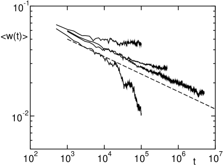
Figure 5: Log-log plot of the space averaged difference variable $w(t)$ as a function of time for two coupled CML’s (see text) and for different coupling values: from lower to upper, the full lines correspond to $\sigma=0.178$, $\sigma=0.17756$, $\sigma=0.1775$, $\sigma=0.177$, while the long dashed line marks the power low expected for the DP critical behaviour. Numerical data have been obtained averaging over $100$ realizations of a CML of size $L=2^{17}$.

The crucial difficulty to determine the universality class for the synchronization transition is that the order parameter (the difference field) can be arbitrarily small. This casts doubts about the very definition of the zero-difference field as a truly absorbing state. In fact, in a previous paper GLP02 , it was speculated that the DP scaling behaviour might be restricted to a finite range. The analysis carried on in this paper clarifies that the synchronization transition genuinely belongs to DP universality class: this has been understood from an objective identification of the threshold $W_{c}$ below which the dynamics is really controlled by linear mechanisms and thus corresponds to an effective contraction. The parametrization of $\tau(W)$ introduced to describe the single-map case has greatly helped to unveil the overall scenario since it has clarified that the basic effect of the diffusive coupling is to renormalize the parameters defining $\tau(W)$ (see Eq. (47)). Here, the parameter values (in particular $W_{c}$) have been inferred by fitting the numerical data; in the future, it will be desirable to find an analytic, though approximate, way of performing the renormalization.

Once we have concluded that synchronization arises through a DP-like transition in a finite parameter region, it is natural to ask how this scenario crosses over to the standard transition characterized by a vanishing of the Lyapunov exponent and by the KPZ critical exponents. With reference to Fig. 1, this question amounts to investigating the region around the multicritical point $\Delta_{c}$. A purely numerical analysis of this region is not feasible in this model, as it would require considering too large systems to be effectively handled. We are currently studying this problem in a different context, where preliminary studies indicate the possibility to draw quantitative conclusions.

Finally, since it is known that finite-size Lyapunov exponents do depend on the norm, it might be worth considering $q$ values different from 1, in order to check to what extent the universality of the transition is preserved when different averaging procedures are adopted to assess the amplitude of the global perturbation. In particular, since $q=\infty$ (corresponding to the maximum norm) takes care only of the extreme fluctuations of a perturbation field, it is not totally obvious that the behaviour of the corresponding first passage time follows exactly the above described scenario.

Appendix A First passage times in the discontinuous uncoupled RM model

In this appendix we report the analytical calculation of the first passage time when $\varepsilon=0$ and $\Delta=0$, to prove Eq. (42). Being $W_{n}=a^{n}$ and $w(0)=1$, we have also $\tau(W_{0})=0$. In order to compute the first passage time through a threshold $W_{n}$, we need to know the average time needed to pass from $W_{n-1}$ to $W_{n}$. With a probability $1-aW_{n-1}$, this can occur in one time step, if the amplification mechanism is not activated and the synchronization error is contracted by a factor $a$. On the other hand, with probability $aW_{n-1}$, the amplification resets the state variable to the value 1. In this case, one has to wait for the synchronization error to shrink back to the $n$-th threshold, which, by definition, occurs in an average time $\tau_{n-1}$. At this point, the error can either shrink to $W_{n}$ or be reset again to 1, to start again the process. Altogether,

$$\tau(W_{n})= \tau(W_{n-1})+1\cdot(1-aW_{n-1})+(2+\tau(W_{n-1})(1-aW_{n-1})aW_{n-1}+$$ (58)

$$(3+2\tau(W_{n-1})(1-aW_{n-1})(aW_{n-1})^{2}+\ldots$$

$$=\tau(W_{n-1})+(1-aW_{n-1})\sum_{i=0}^{\infty}\left[(1+i+i\tau(W_{n-1}))(aW_{n-1})^{i}\right]$$

$$=\tau(W_{n-1})+(1-a^{n})\left[\sum_{i=0}^{\infty}(a^{n})^{i}+(\tau(W_{n-1}+1)\sum_{i=0}^{\infty}i\,(a^{n})^{i}\right]\quad.$$

Summing up the series, one obtains

$$\tau(W_{n})=\frac{\tau(W_{n-1})+1}{1-a^{n}}\quad.$$ (59)

References

- (1) A. Pikovsky, M. Rosenblum and J. Kurths, Synchronization : A Universal Concept in Nonlinear Sciences, Cambridge University, Press, Cambridge (2002).
- (2) S. Fahy and D.R. Hamann, Phys. Rev. Lett. 69, 761 (1992).
- (3) A. Maritan and J. R. Banavar, Phys. Rev. Lett. 72, 1451 (1994) and 73, 2932 (1994).
- (4) A. S. Pikovsky, Phys. Rev. Lett. 73, 2931 (1994).
- (5) H. Herzel and J. Freund, Phys. Rev. E 52, 3238 (1995).
- (6) C.H. Lai and Changsong Zhou, Europhys. Lett. 43, 376 (1998).
- (7) A. S. Pikovsky, Phys. Lett. A 165, 33 (1992).
- (8) L. Baroni, R. Livi, and A. Torcini, Phys. Rev. E 63, 036226 (2001).
- (9) V. Ahlers and A. Pikovsky, Phys. Rev. Lett. 88 254101 (2002).
- (10) G. Grinstein, M. A. Muñoz, and Y. Tu, Phys. Rev. Lett. 76, 4376 (1996).
- (11) Having in mind to work with discrete-time systems, it is natural to adopt the Itô interpretation.
- (12) J. Marro and R. Dickman, Nonequilibrium Phase Transitions in Lattice Models, Cambridge University Press, Cambridge, England (1999);
- (13) P. Grassberger, Directed Percolation: Results and Open Problems, in Nonlinearities in Complex Systems, Prooceedings of 1995 Shimla Conference on Complex Systems, eds. S. Puri et al. (Narosa Publishing, New Dehli, 1997).
- (14) H. Hinrichsen, Advances in Physics 49, 815 (2000).
- (15) F. Ginelli, R. Livi, and A. Politi, J. Phys. A 35, 499 (2002).
- (16) E. Domany and W. Kinzel, Phys. Rev. Lett. 53, 311 (1984).
- (17) This is indeed true for coupled Bernoulli maps , even though the diffusive coupling induces some inhomogeneity in the flat distribution of the single map.
- (18) M.A. Muñoz, Phys. Rev. E 57, 1377 (1998).
- (19) A. U. Neumann and B. Derrida, J. Phys. France 49, 1647 (1988).
- (20) I. Jensen, J. Phys. A 29, 7013 (1996); I. Jensen, J. Phys. A 32, 5233 (1999).
- (21) Y. Tu, G. Grinstein and M. A. Muñoz Phys. Rev. Lett. 78, 274 (1997).
- (22) R. Kubo, M. Toda and N. Hashitsume, Statistical physics II: nonequilibrium statistical mechanics, vol 31 of Springer Series in Solid-State sciences, Springer-Verlag, Berlin (1985).
- (23) E. Aurell, G. Boffetta, A. Crisanti, G. Paladin and A. Vulpiani, Phys. Rev. Lett. 77, 1262 (1996) and J. Phys. A30, 1 (1997).
- (24) M. Cencini and A. Torcini, Phys. Rev. E 63 056201 (2001).
- (25) A. Politi and A. Torcini, Europhys. Lett. 28, 545 (1994).
- (26) Notice that plays here the same role as in the RM.
- (27) A. Politi and A. Torcini, Chaos 2, 293 (1992);
- (28) S. Lepri, A. Politi and A. Torcini, J. Stat. Phys. 82, 1429 (1996).