CONSTRAINT SATISFACTION BY SURVEY PROPAGATION

Abstract

Survey Propagation (SP) is an algorithm designed for solving typical instances of random constraint satisfiability problems. It has been successfully tested on random $3$-satisfiability (3-sat) and random ${\cal G}(n,\frac{c}{n})$ graph $3$-coloring (3-col), in the hard region of the parameter space, relatively close the the SAT/UNSAT phase transition. Here we provide a generic formalism which applies to a wide class of discrete Constraint Satisfaction Problems.

I Introduction

In this paper we suggest a new theoretical framework for the so called “Survey Propagation” (SP) equations that are at the root of both the analysis and the algorithms used in ref. MEPAZE ; MZ_pre ; nosotros ; Coloring to solve the random 3-Sat and q-Coloring problems. In the more general context of constraint satisfaction problems we propose a slightly different way of deriving the equations which we hope can shed some light on the potentialities of the algorithms and which makes clear the differences with other well known iterative probabilistic algorithms. This line of approach, also discussed in GP for the satisfiability problem, is developed here systematically through the addition of an extra state for the variables which allows to take care of the clustered structure of the space of solutions. Within clusters a variable can be either “frozen” to some value – that is, the variable takes always the same value for all solutions (satisfying assignments) within the cluster – or it may be “unfrozen” – that is it fluctuates from solution to solution within the cluster. As we shall discuss, scope of the SP equations is to properly describe the cluster to cluster fluctuations by associating to unfrozen variables an extra state to be added to those belonging to the original definition of the problem. The overall algorithmic strategy is iterative and decomposable in two elementary steps: First, the marginal probabilities of frozen variables are evaluated by the SP message-passing procedure; Second – the so called decimation step – using such information some variables are fixed and the problem is simplified. While the first step is unavoidable if one is interested in marginal probabilities, the second step is just dictated by simplicity and we expect that there could exist other ways of efficiently using the information provided by the marginals.

Throughout the paper, a detailed comparison with a similar message-passing procedure, Belief Propagation, which does not make assumptions about the structure of the solution space will also be given.

The structure of the paper is as follows. In Sec. II, we provide the general formalism, namely the definitions of Constraint Satisfaction Problems, Factor Graphs and Cavities, with concrete reference to the cases of Coloring and Satisfiability. In Sec. III, we introduce the warnings and the local fields whose histograms will provide the so called Belief Propagation equations. Finally in Sec. IV, clusters are introduced and the SP equations are derived. Explicit equations are given for both 3-col and 3-sat and the decimation procedure is discussed.

II Generalities

II.1 Constraint satisfaction problems

We consider a constraint satisfaction problem (CSP) which is defined on a set of discrete variables $\vec{x}=\left(x_{i}\right){}_{i\in I}$ with $I=\left\{1,\dots,n\right\}$. Each variable $x_{i}$ can be in $q$ possible states (the generalization to the case where the number of states is $i-$ dependent is straightforward), so $\vec{x}\in X=\left\{1,\dots,q\right\}{}^{n}$. The vector $\vec{x}$ is called a configuration. These variables are subject to a set of constraints $\{C_{a}\}_{a\in A}$. Each $C_{a}$ depends on $\vec{x}$ only through a subset $(x_{i})_{i\in I(a)}$ of variables. It is defined as a mapping $C_{a}:\left\{1,\dots,q\right\}^{|I(a)|}\to\{0,1\}$, where the value $C_{a}=0$ zero corresponds to a satisfied constraint, and $C_{a}=1$ to an unsatisfied constraint. It is useful to introduce, for every $i\in I$, the subset $A(i)\subset A$ of indices of all constraints involving $x_{i}$. The index sets $I$ and $A$ are chosen disjoint, so that their elements uniquely determine a single variable or constraint.

We define the cost function

$$C[\vec{x}]=\sum_{a\in A}C_{a}[\left(x_{i}\right)_{i\in I(a)}]$$ (1)

which counts the number of unsatisfied constraints. Our goal is to simultaneously satisfy all constraints, i.e. to find a configuration $\vec{s}\in X$ with $C[\vec{s}]=0$. We thus introduce the subset $S_{C}\subset X$ of solutions to our CSP instance as

$$S_{C}=\{\vec{s}\ |\ \vec{s}\in X,\ C[\vec{s}]=0\}\ .$$ (2)

The algorithm aims at finding one solution $\vec{s}\in S_{C}$. We concentrate a priori onto instances $C[\vec{x}]$ which possess a non-empty solution set $S_{C}$.

II.2 Factor graph

We use the factor-graph factor_graph representation for a CSP:

Definition II.1

For any instance of the CSP problem, we define its factor graph as a bipartite undirected graph $G=\left(V,E\right)$, having two types of nodes:

• variable nodes $i\in I$ and

• function nodes $a\in A$.

Edges connect only different node types; the edge $\left(i,a\right)$ belongs to the graph if and only if the constraint $C_{a}$ involves the variable $x_{i}$, i.e. if $a\in A\left(i\right)$ or equivalently $i\in I\left(a\right)$. More formally, we define $V=A\cup I$ and $E=\left\{(i,a)\ |\ i\in I,a\in A(i)\right\}=\left\{(i,a)\ |\ a\in A,i\in I(a)\right\}$.

In figures, we always represent variable nodes by circles, whereas function nodes are drawn as squares. This notation will help to distinguish between the different origins of the two node types.

II.3 Cavities

Given a CSP and its factor graph, we will use the cavity graphs obtained by removing a variable:

Definition II.2

Given a factor graph $G$ and one variable node $i\in I$, we define the cavity graph $G^{(i)}$ by deleting from $G$ all function nodes $a\in A(i)$ which are adjacent to $i$, and the edges incident to these function nodes.

The cavity graph $G^{(i)}$ defines a new CSP, where the cost function is

$$C^{(i)}=C-\sum_{a\in A(i)}C_{a}=\sum_{b\notin A(i)}C_{b}\ .$$ (3)

Note that in this new problem the variable $x_{i}$ is isolated, it can take any value without violating a constraint. The solution set $S^{(i)}$ for the cavity problem $G^{(i)}$ is larger than the original one, since some constraints have been removed.

II.4 Two examples: Satisfiability and Coloring

Although the algorithm can in principle be written for arbitrary CSP, we shall present two specific examples, satisfiability and coloring.

In the satisfiability problem a constraint $C_{a}$ is a clause, which is unsatisfied by only one assignment of the variables $(x_{i})_{i\in I(a)}$. In the random 3-SAT problem each clause involves three variables ($|I(a)|=3$), the indices of which are chosen randomly with uniform distribution in $I$. For a given $a$ and $I(a)$, there are eight different types of constraints $C_{a}$, corresponding to the combinations of possible negations of literals in one clause, see Fig. 1. In random 3-SAT the type of clauses is chosen with uniform distribution among these eight types.

In the $q$-coloring problem one is given an original undirected graph. The problem is to color the vertices, using $q$ colors, so that two vertices connected by an edge have different colors. There is one constraint associated with each edge of the original graph, and the factor-graph appears as a decoration of the original graph (see Fig.2), where function nodes have been added on each original edge. There is only one type of function node. In the random $q$-col problem, the original graph is a random ${\cal G}(n,\frac{c}{n})$ graph.

We will be particularly interested in the behavior of the algorithm for large $n$. Note that both $K$-SAT and $q$-col are problems where $|A(i)|$ have a Poisson limit distribution with finite mean when $n\to\infty$, i.e. $|A(i)|$ is typically much smaller than $n$. Moreover, the structure of the factor graph is locally tree-like. This will guide us in the definition of the algorithm below, and it is presumably an important ingredient for the algorithm to work.

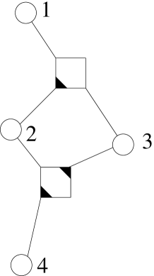
Figure 1: The factor graph of a 3-SAT problem corresponding to the simple formula: $\left(x_{1}\vee\overline{x}_{2}\vee x_{3}\right)\wedge\left(x_{2}\vee\overline{x}_{3}\vee\overline{x}_{4}\right)$. Variables are represented as circles, clauses (i.e. function nodes) as squares. A triangle-shaped mark indicates that the corresponding literal is negated

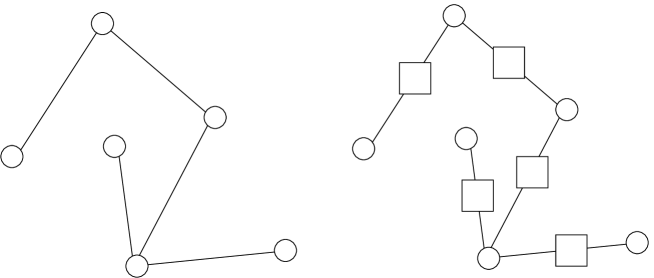
Figure 2: The original graph (left) and its factor graph (right) corresponding to a coloring problem

III Belief propagation

III.1 Warnings and fields

Given a CSP and a configuration $\vec{x}\in X$, we define the following three quantities associated with $\vec{x}$, cf. MZ_pre ; nosotros :

Definition III.1

For a given edge $a-i$ of the factor graph, with $i\in I$ and $a\in A\left(i\right)$, we define a warning as the $q$-component vector $\vec{u}_{a\to i}(\vec{x})\in\left\{0,1\right\}^{q}$ with components:

$$u_{a\to i}^{p}(\vec{x})=C_{a}\left[(x_{j})_{j\in I(a)}\ |\ x_{i}\leftarrow p\right]\ ,\ p=1,...,q,$$

So $u_{a\to i}^{p}(\vec{x})$ is the value of constraint $C_{a}$ in the configuration obtained from $\vec{x}$, by substituting $p$ in the place of $x_{i}$.

Definition III.2

For a given edge $a-i$ of the factor graph, with $i\in I$ and $a\in A\left(i\right)$, we define a cavity field as the $q$-component vector $\vec{h}_{i\to a}(\vec{x})\in\{0,1\}^{q}$ with components:

$$h_{i\to a}^{p}(\vec{x})=\max_{b\in A(i)\setminus a}u_{b\to i}^{p}(\vec{x})$$

Definition III.3

For a given node $i\in I$, we define the local field as the $q$-dimensional vector $\vec{h}_{i}(\vec{x})\in\{0,1\}^{q}$ with components:

$$h_{i}^{p}(\vec{x})=\max_{a\in A(i)}u_{a\to i}^{p}(\vec{x})\ .$$

The warning ${\vec{u}}_{a\to i}(\vec{x})$ is understood as a message sent from constraint $a$ to variable $i$ saying: $x_{i}$ cannot be in any of the states $p$ where $u_{a\to i}^{p}(\vec{x})=1$, without violating constraint $a$. Note that we do not need the value of $x_{i}$ for computing $\vec{u}_{a\to i}$. In fact, the warning depends explicitly only on $(x_{j})_{j\in I(a)\setminus i}$.

The local field on variable $i$ summarizes all warnings sent to $i$ from the constraints, i.e. $h_{i}^{p}(\vec{x})\neq 0$ means that, given the values of all other variables $(x_{j}),j\neq i$, the variable $x_{i}$ should not be assigned the value $p$, because at least one neighboring constraint would be violated.

The cavity field ${\vec{h}}_{i\to a}(\vec{x})$ summarizes all warnings sent to $i$ from the constraints different from $a$.

III.2 Histograms

The elementary messages above are defined for an arbitrary configuration $\vec{x}$. We are eventually interested in knowing, for each variable $i$, the histogram of local fields for the configurations which are solutions of the CSP:

$$H_{i}(\vec{h})=\frac{1}{|S_{C}|}\sum_{\vec{s}\in S_{C}}\delta_{\vec{h},\vec{h}_{i}(\vec{s})}\ ,$$ (4)

where the ($q$-dimensional) Kronecker-Delta is simply denoted by $\delta$. This histogram can also be interpreted as probability distributions $H_{i}(\vec{h})=Prob(\vec{h}_{i}(\vec{s})=\vec{h}\ |\ \vec{s}\in S_{C})$ of local fields for randomly chosen solutions.

Local-field histograms contain useful information about the set $S_{C}$ of solutions, which can be exploited algorithmically in order to recursively construct one solution. If, e.g., one of the field components is non-zero for all solutions $\vec{s}\in S_{C}$, this particular state is forbidden to this variable. If all but one components are non-zero, the variable is “frozen” to one specific value in all solutions, i.e. it belongs to the so-called backbone, and it can be assigned right away.

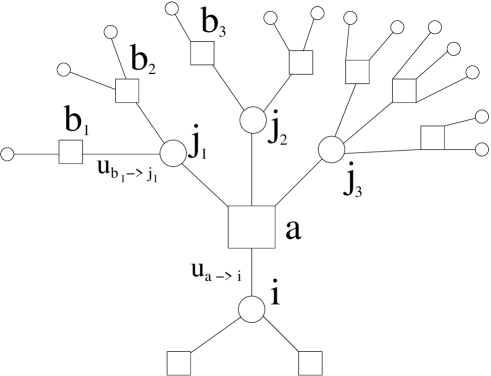
Figure 3: Iteration for $\vec{u}$ warnings.

Computing $H_{i}(\vec{h})$ is a difficult task, but one may compute it approximately using a message passing procedure. We first try to find a recursion relation for the related histograms of the warnings $\vec{u}_{a\to i}(\vec{s})$ over all solutions $\vec{s}\in S_{C}$ nosotros . Considering Fig. 3 as an example, we note that the histogram of $\vec{u}_{a\to i}(\vec{s})$ depends on the joint histogram of all the warnings $\vec{u}_{b\to j}(\vec{s})$ sent to all variables $j\in\{j_{1},j_{2},j_{3}\}$“above” function node $a$ (we call them the incoming warnings). The obvious problem is that this joint distribution is not known. If the $\vec{u}_{b\to j}(\vec{s})$ were independent variables, we would be able to factorize the joint histogram into the product of all individual histograms of warnings $\vec{u}_{b\to j}(\vec{s})$, and then to obtain a recursion. But in general there is no reason for them to be independent. Moreover, they cannot even be approximately independent as there are very short paths joining variables “above” variable nodes $j$ (the small unnamed ones in the figure) between them, variables which in turn define the $\vec{u}_{b\to j}(\vec{s})$ messages. This is where the cavity graph is useful.

For each edge $a-i$ of the factor graph, we define the belief $B_{a\to i}(\vec{u})$ as the histogram of the warning $\vec{u}_{a\to i}$ over the configurations $s\in S^{(i)}$ which are solutions of the cavity graph problem:

$$B_{a\to i}(\vec{u}) = \frac{1}{|S^{(i)}|}\sum_{\vec{s}\in S^{(i)}}\delta_{\vec{u},\vec{u}_{a\to i}(\vec{s})}$$ (5)

$$= Prob\left(\vec{u}_{a\to i}(\vec{s})=\vec{u}\ |\ \vec{s}\in S^{(i)}\right)\ ,$$

where the second line refers again to the probabilistic interpretation: $B_{a\to i}(\vec{u})$ describes the probability of finding a warning $\vec{u}$ if a solution of the cavity graph is randomly selected.

III.3 Belief propagation equations

Look again at Fig.3: If the factor graph $G$ is a tree, vertices above $j_{1},j_{2}$ and $j_{3}$ become disconnected if function nodes $b_{i}$ are removed, and the various messages $\vec{u}_{b\to j}$ are uncorrelated. In this case, we can thus determine the belief $B_{a\to i}$ as a function of all the incoming beliefs (i.e. the histograms of the incoming warnings $\{B_{b\to j}\}$ with $j\in I\left(a\right)\setminus i$ and $b\in A\left(j\right)\setminus a$), and so on recursively for the full factor graph. Standard belief propagation uses this same recursion also in more general factor graphs with loops, as a means to compute approximately the local-field histograms and the beliefs (see e.g. YedFreeWei ).

In order to write the corresponding ’belief propagation’ equations explicitly, we use notations similar to those of Fig.3. Given the edge $a-i$ connecting the function node $a$ to the variable $i$, we denote by $J$ the set of indices of the variable nodes “above” the function node $a$, i.e. $J=I\left(a\right)\setminus i$ (in the figure $J=\{j_{1},j_{2},j_{3}\}$). For each $j\in J$, we denote by $D_{j}=A\left(j\right)\setminus a$ the set of function node “above” the variable $j$ (in the figure, $D_{j_{1}}=\{b_{1},b_{2}\}$, and by $\hat{D}$ the union of these sets: $\hat{D}=\bigcup_{j\in}D_{j}$). The “incoming messages”, which can be warning or beliefs, are all the messages propagated on the edges $b\to j$ with $j\in J$ and, for each such $j$, $b\in D_{j}$.

Let us first consider a set of incoming warnings $\{\vec{u}_{b\to j}\}$. This warning set may or may not be “extensible” to a configuration $(s_{j})_{j\in J}$ satisfying all constraints $(C_{b})_{b\in\hat{D}}$. One can easily go through a bureaucratic procedure to evaluate all configurations $(s_{j})_{j\in J}$ compatible with the warning set. First compute the cavity fields III.3 component-wise: $h_{j\to a}^{p}=\max_{b\in D_{j}}(u_{b\to j}^{p})$. For each $j\in J$, the allowed values of $s_{j}$ are those such that $h_{j\to a}^{s_{j}}=0$. We denote by $T(\{\vec{h}_{j\to a}\})\subset\{1,...,q\}^{|J|}$ the set of allowed configurations of the $s_{j}$ variables:

$$T(\{\vec{h}_{j\to a}\})=\left\{(s_{j})_{j\in I(a)\setminus i}\ |\ h_{j\to a}^{s_{j}}=0,\ \forall j\in I\left(a\right)\setminus i\right\}$$ (6)

For each $(s_{j})$ in $T(\{\vec{h}_{j\to a}\})$, one can determine the output warning $\vec{u}_{a\to i}$ using definition III.1.

This procedure can be embedded into the probabilistic description of solutions on the cavity graph. For doing so, we assume that incoming warnings are independent. Following the steps above, one first calculates from the incoming beliefs the distributions of cavity fields

$$H_{j\to a}(\vec{h})=\sum_{\{\vec{u}_{b\to j}\}_{b\in D_{j}}}\delta_{\vec{h},\vec{h}_{j\to a}}\prod_{b\in D_{j}}B_{b\to j}(\vec{u}_{b\to j})\ .$$ (7)

The new distribution of warnings $\vec{u}_{a\to i}$ is now given by an average over cavity fields,

$$B_{a\to i}(\vec{u})={\cal Z}^{-1}\sum_{\{\vec{h}_{j\to a}\}_{j\in J}}\left[\sum_{\vec{s}\in T(\{\vec{h}_{j\to a}\})}\delta_{\vec{u},\vec{u}_{a\to i}(\vec{s})}\right]\prod_{j\in J}B_{j\to a}(\vec{h}_{j\to a})$$ (8)

The prefactor ${\cal Z}^{-1}$ is a normalization constant. Note that each cavity-field configuration $\{\vec{h}_{j\to a}\}$ is contributing $|T(\{\vec{h}_{j\to a}\})|$ terms. As a byproduct, contradictory messages automatically do not contribute anything to (8).

The BP equations (7,8) are equivalent to the so called sum-product (or belief network, or Bayesian network) equations Gallager ; pearl . One can try to solve them by iteration, starting form some randomly chosen beliefs, and updating $B_{a\to i}$ sequentially on randomly chosen $a-i$ edges. In some cases, the iteration converges, independently of the scheme of updating, to a unique solution. When the belief propagation equations converge, one can use the obtained beliefs in order to estimate the histogram of local fields, using:

$$H_{j}(\vec{h})\simeq\sum_{\{\vec{u}_{b\to j}\}_{b\in A(j)}}\delta_{\vec{h},\vec{h}_{j\to a}}\prod_{b\in A(j)}B_{b\to j}(\vec{u}_{b\to j})\ .$$ (9)

and this histogram can be used for decimation.

III.4 An example of Belief Propagation: 3-COL

For the sake of clarity, let us work out BP on a simple example of the 3-col problem ($q=3$), see Fig. 4. Since function nodes are connected to two variable nodes only (constraints are edges in the original graph), there is only one variable node $j$ above function node $a$. For a given configuration of incoming warnings $\left\{\vec{u}_{b\to j}\right\}$, we can make a table of allowed states $s_{j}$, and for each of them, we can compute the outgoing warning $\vec{u}_{a\to i}(s_{j})$. Note that possible warnings are $(1,0,0)$, $(0,1,0)$, $(0,0,1)$, since a function node can only forbid one color (which is given by the state of the other variable connected to the function node).

• Suppose that $\vec{u}_{b_{1}\to j}=(1,0,0)$, $\vec{u}_{b_{2}\to j}=(0,1,0)$, and $\vec{u}_{b_{3}\to j}=(0,0,1)$. Then $h_{j\to a}=(1,1,1)$, we find a contradictory message. No satisfiable configuration exists for $s_{j}$. According to the procedure given above, this configuration does not contribute.

• Suppose that incoming messages are $\vec{u}_{b_{1}\to j}=\vec{u}_{b_{2}\to j}=(1,0,0)$, and $\vec{u}_{b_{3}\to j}=(0,1,0)$. Then $h_{j\to a}=(1,1,0)$, and the only possible coloring state for $j$ is $s_{j}=3$. For this configuration, we thus have only one possible outgoing warning, $\vec{u}_{a\to i}=(0,0,1)$.

• If $\vec{u}_{b_{1}\to j}=\vec{u}_{b_{2}\to j}=\vec{u}_{b_{3}\to j}=(1,0,0)$, then $h_{j\to a}=(1,0,0)$, and there are two possible colors for $s_{j}$, namely states $2$ and $3$. For the first one we have $u_{a\to i}=(0,1,0)$, and for the second one $u_{a\to i}=(0,0,1)$. Both contribute with equal weight to $B_{a\to i}$.

• All other configurations are simple color permutations of the three cases mentioned above, and are handled analogously.

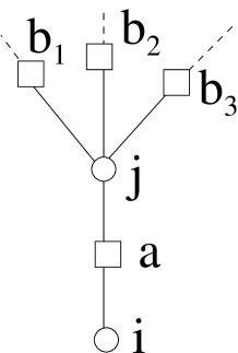
Figure 4: An example of the coloring problem. This part of the factor graph is the one necessary to compute the messages (warning and belief) passed from the function node $a$ to the variable node $i$.

From Eqs. (7,8), we can easily deduce the equation giving the probability distribution $B_{a\to i}$ in terms of all distributions $\{B_{b_{l}\to j};l=1,2,3\}$. Parameterizing $B_{a\to i}$ according to the three possible messages as

$$B_{a\to i}(\vec{u})=\eta_{a\to i}^{1}\delta_{\vec{u},(1,0,0)}+\eta_{a\to i}^{2}\delta_{\vec{u},(0,1,0)}+\eta_{a\to i}^{3}\delta_{\vec{u},(0,0,1)}\ ,$$ (10)

we find

$$\eta_{a\to i}^{p}=\frac{\prod_{l=1}^{3}(1-\eta_{b_{l}\to j}^{p})}{\sum_{r=1}^{q}\prod_{l=1}^{3}(1-\eta_{b_{l}\to j}^{r})}$$ (11)

This expression can be easily understood: $\eta_{a\to i}^{p}$ equals the probability that color $p$ is forbidden for node $i$, which means that node $j$ has already taken this color, $s_{j}=p$. Now, node $j$ can take color $p$ if and only if it is not forbidden by any incoming warning: The numerator in Eq. (11) simply calculates the probability that none of the incoming messages forbids color $p$, the denominator guarantees normalization. Note that configurations in which all variables above $j$ take the same color $r$, are counted twice, namely in the expressions for both $p\neq r$. According to the general discussion given above, this is correct because we have two new configurations for $s_{j}$, and two corresponding messages $\vec{u}_{a\to i}$ can be sent.

Due to the symmetry between colors, a possible solution would be $\eta_{a\to i}^{p}=1/q$ for all edges $(i,a)\in E$ and all colors $p$. Note, however, that the main intention is to use these equations in a recursive coloring algorithm. This means, some variable nodes may already be assigned a color before, which explicitly breaks the symmetry. Still, Eq. (11) is valid.

IV Survey propagation

IV.1 Clustering

Pitifully, the Belief Propagation dynamics is known not to converge for the random version of many combinatorial problems (including again $3$-sat and $q$-col) in the region of the parameters near the SAT/UNSAT threshold. Recently, using tools from statistical physics, it has been possible to reach some understanding of what happens in the solution space of these problems around this threshold MEPAZE ; MZ_pre ; cavity . Well below the threshold, i.e. where the number $|A|/n$ of constraints per variable is relatively small, a generic problem has exponentially many solutions, which tend to form one giant cluster: For any two solutions, it is possible to find a connecting path via other solutions that requires short steps only (each pair of consecutive assignments in the path is close together in Hamming distance).

Close to the critical threshold, however, the solution space breaks up into many smaller clusters. Solutions in separate clusters are generally far apart. In addition, the cost function $C[\vec{x}]$ has exponentially many local minima, separated from each other by large cost “barriers”. These local cost minima are exponentially more numerous than the solution clusters, and they act as traps for local search algorithms.

According to the statistical-physics analysis (which considers the infinite size limit, $n\to\infty$), there exist exponentially many widely separated clusters of solutions. Within one such cluster of solutions, we may identify two types of variables: those which are frozen in one single state, for all configurations belonging to the cluster, and those – unfrozen – which fluctuate from solution to solution inside the cluster. Note that also the variables which are frozen within one solution cluster may change their state when we go to another cluster, there they may even be unfrozen. While in general the above distinction can only provide an approximate description of clusters, it appears from numerical experiments that in many hard random CSP, like $K$-sat or $q$-col, such type of approximation is already rather accurate.

IV.2 The joker states

Survey propagation turns out nosotros to be able to deal with this clustering phenomenon for large (finite) sizes $n$. Although the original derivation uses sophisticated statistical physics ideas, one can also develop it more directly in algorithmic terms. The main idea is that we do not work any more with individual solutions $\vec{s}\in S_{C}$, but with complete clusters of solutions. As already said, some variables may be frozen inside a cluster, so they retain one single value $s_{j}\in\{1,...,q\}$ in our description. Other variables may take several values n the cluster. For handling these variables, one can introduce an additional joker state which we denote by a “$\star$”. An even finer description, useful for general CSP, uses varieties of joker states, describing the set of values which are allowed for the variable, so that $s_{j}\in{\cal P}$, where $\cal P$ is the ensemble built from all subsets of $\{1,...,q\}$. To each cluster one should associate exactly one generalized value of each variable. One can then generalize the constraint to this enlarged space and work out the corresponding belief propagation equations. The resulting equations are the survey propagation equations.

We shall not develop in more details this ’derivation’, since it does not give any rigorous construction, but we will directly write the equations themselves, in terms of the original variables $\vec{x}\in\{1,...,q\}^{n}$, and then analyze them.

IV.3 Generalized messages

We first need to define the generalizations of the warnings, the cavity-fields and the local field used in survey propagation. In order to lighten the notation and presentation, we shall drop the ’generalized’, and use the same notation for generalized warning as we used for warnings in the BP section. The reader should remember that in SP all the messages are ’generalized’ messages.

For a given CSP, we define the generalized warnings:

Definition IV.1

For a given edge $a-i$ of the factor graph, with $i\in I$ and $a\in A\left(i\right)$, let $S$ be a given set of possible values for the variables $(x_{j})_{j\in I(a)\setminus i}$ which are ‘above’ $a$. We define the warning as the $q$-component vector $\vec{\hat{u}}_{a\to i}(\vec{x})\in\left\{0,1\right\}^{q}$ with components:

$$\hat{u}_{a\to i}^{p}(S)=\min_{(x_{j})\in S}C_{a}\left[(x_{j})_{j\in I(a)\setminus i}|\ x_{i}\leftarrow p\right]\ ,\ p=1,...,q,$$

(The generalized warning was called cavity-bias in MZ_pre ). Note that the set of possible warnings is enlarged in SP: For the example of 3-col the null message $(0,0,0)$ is added to $(0,0,1)$, $(0,1,0)$ and $(1,0,0)$. As we have discussed before, the non-null messages are sent if the node “above” a function node is assigned a fixed color in the solution cluster. Correspondingly, the new message is sent if this vertex is not fixed to a single color, i.e. if it is in the joker state.

Based on these warnings, we define local and cavity fields according to Def. III.3, with the argument (a single configuration) replaced by a set $S$ of configurations:

$$h_{i}^{p}(S) = \max_{a\in A(i)}u_{a\to i}^{p}(S)\ ,$$

$$h_{j\to a}^{p}(S) = \max_{b\in A(j)\setminus a}u_{b\to j}^{p}(S)\ .$$ (12)

IV.4 Histograms

Histograms of warnings and fields are now defined as sums over clusters. The histogram of local fields is given by

$$H_{i}(\vec{h})=\frac{1}{n_{cl}}\sum_{\alpha=1}^{n_{cl}}\delta_{\vec{h},\vec{h}_{i}(S_{C}^{\alpha})}\ .$$ (13)

The histogram of the generalized warning on an edge $a-i$ is now called the survey, denoted $Q_{a\to i}(\vec{u})$. It is defined in terms of the clusters of solutions for the cavity graph where $i$ has been taken away. Calling $S_{C}^{\alpha,(i)}$ the corresponding clusters, and $n_{cl}^{(i)}$ their numbers, one defines:

$$Q_{a\to i}(\vec{u})=\frac{1}{n_{cl}^{(i)}}\sum_{\alpha=1}^{n_{cl}^{(i)}}\delta_{\vec{u},\vec{u}_{a\to i}(S_{C}^{\alpha,(i)})}\ .$$ (14)

IV.5 Survey propagation equations

Based on these definitions, one can easily guess the generalized recurrence equations for the (approximate) probabilities $Q_{a\to i}(\vec{u})$ that implement the solutions in this enlarged configuration space. These SP equations lead to a small, yet fundamental, modification of the BP equations. The basic assumption is again, that incoming warnings are independent. But contradictory messages have to be explicitly forbidden. Having Fig. 3 in mind, and using the same notations as in sect.III.3, we use the incoming surveys (i.e. the set of surveys: $\{Q_{b\to j}\}$ with $j\in I\left(a\right)\setminus i$ and $b\in A\left(j\right)\setminus a$) to calculate the cavity-field distributions as in (7):

$$H_{j\to a}(\vec{h})=\sum_{\{\vec{u}_{b\to j}\}_{b\in D_{j}}}\delta_{\vec{h},\vec{h}_{j\to a}}\prod_{b\in A(j)\setminus a}Q_{b\to j}(\vec{u}_{b\to j})\ .$$ (15)

Remember that these fields may lead to contradictions, if and only if $\vec{h}_{j\to a}=(1,1,...,1)$ for at least one $j$. We therefore introduce the set of all non-contradictory cavity field configurations,

$${\cal M}_{a\to i}=\left\{\{\vec{h}_{j\to a}\}_{j\in I(a)\setminus i}\ |\ \forall j:\ \vec{h}_{j\to a}\in\{0,1\}^{q},\ \vec{h}_{j\to a}\neq(1,...,1)\ \right\}\ .$$ (16)

Then, for an element of ${\cal M}_{a\to i}$ we define again

$$T\left(\{\vec{h}_{j\to a}\}\right)=\left\{(s_{j})_{j\in I(a)\setminus i}\ |\ h_{j\to a}^{s_{j}}=0,\ \forall j\in I(a)\setminus i\right\}\ ,$$ (17)

the set of allowed configuration for the variable nodes above function node $a$. Now the difference to BP enters: All elements of $T(\{\vec{h}_{j\to a}\})$ naturally belong to the same cluster, i.e. they give rise to a single outgoing warning! The new warning is thus computed on the set of allowed configurations, it is given by $\vec{u}_{a\to i}(T(\{\vec{h}_{j\to a}\}))$. Its distribution follows immediately,

$$Q_{a\to i}(\vec{u})=\tilde{\cal Z}^{-1}\sum_{\{\vec{h}_{j\to a}\}\in{\cal M}_{a\to i}}\delta_{\vec{u},\vec{u}_{a\to i}\left(T(\{\vec{h}_{j\to a}\})\right)}\prod_{j\in I(a)\setminus i}H_{j\to a}(\vec{h}_{j\to a})\ .$$ (18)

The equations (15,18) are the SP equations. Note that Eq. (18) produces a dramatic change in the iteration of the probabilities with respect to the BP Eq. (8): Every allowed cavity-field configuration contributes only one term to the sum. Note also that contradictory messages have to be excluded explicitly by summing only over ${\cal M}_{a\to i}$. In belief propagation, for each configuration of input messages one takes the full collection of possible outputs, thereby introducing a bifurcation mechanism (which may easily become unstable). On the contrary, in SP the presence of multiple outputs is collapsed into the null message (which may even not be present in the belief propagation formalism as it happens for the coloring problem). A variable which receives a message having at least two zero components will be “unfrozen” in the corresponding cluster.

The SP equations (15-18) provide a closed set of equation for the surveys. Practically, this recurrence defines a map

$$\Lambda:\left\{{}^{old}Q_{a\to i}\right\}_{a\in A(i)}^{i=1,\dots,n}\mapsto\left\{{}^{new}Q_{a\to i}\right\}_{a\in A(i)}^{i=1,\dots,n}$$ (19)

and we are looking for a fixed point of this map, that will be obtained numerically by starting with some (random) initial $\left\{Q_{a\to i}^{0}\right\}$ and applying $\Lambda$ iteratively:

$$\left\{Q^{SP}_{a\to i}\right\}=\lim_{m\to\infty}\begin{array}[b]{c}m\textrm{ times}\\ \overbrace{\Lambda\circ\cdots\circ\Lambda}\end{array}\left\{Q^{0}_{a\to i}\right\}$$ (20)

Such a fixed point will be called a “self-consistent” set of surveys.

IV.6 An example of Survey Propagation: 3-COL

For the 3-col example, because of the additional null message, the warning distribution now reads Coloring_algo

$$Q_{a\to i}^{SP}(\vec{u})=\eta_{a\to i}^{\star}\delta_{\vec{u},(0,0,0)}+\eta_{a\to i}^{1}\delta_{\vec{u},(1,0,0)}+\eta_{a\to i}^{2}\delta_{\vec{u},(0,1,0)}+\eta_{a\to i}^{3}\delta_{\vec{u},(0,0,1)}\ ,$$ (21)

and the SP equations corresponding to fig.4 are given by

$$\eta_{a\to i}^{p}=\frac{\prod_{l=1}^{3}(1-\eta_{b_{l}\to j}^{p})-\sum_{r\neq p}\prod_{l=1}^{3}(\eta_{b_{l}\to j}^{\star}+\eta_{b_{l}\to j}^{r})+\prod_{l=1}^{3}\eta_{b_{l}\to j}^{\star}}{\sum_{r=1}^{q}\prod_{l=1}^{3}(1-\eta_{b_{l}\to j}^{r})-\sum_{r=1}^{q}\prod_{l=1}^{3}(\eta_{b_{l}\to j}^{\star}+\eta_{b_{l}\to j}^{r})+\prod_{l=1}^{3}\eta_{b_{l}\to j}^{\star}}\ ,$$ (22)

for $p\in\{1,2,3\}$. Then $\eta_{a\to 1}^{\star}$can be computed by normalization, i.e:

$$\eta_{a\to i}^{\star}=1-\left(\eta_{a\to i}^{1}+\eta_{a\to i}^{2}+\eta_{a\to i}^{3}\right)$$ (23)

The interpretation of this equation is again straightforward, for simplicity we explain it just for color 1: Now $\eta_{a\to i}^{1}$ is given by the probability that $s_{j}$ is forced to take value $1$, i.e. by the probability that the cavity field equals $\vec{h}_{j\to a}=(0,1,1)$, conditioned to non-contradictory fields. The numerator calculates the unconditioned probability: The first term excludes $h_{j\to a}^{1}$ which would forbid color 1 to $s_{j}$. The second term takes out fields $(0,h^{2},0)$ and $(0,0,h^{3})$ where $s_{j}$ would be allowed to also take at least one other color. The last term adds again the probability of field $(0,0,0)$ which was subtracted twice in the second term. The denominator realizes the conditioning to non-contradictory fields, i.e. it gives the probability that $\vec{h}_{j\to a}\neq(1,1,1)$. The counting of possible cases follows again the inclusion-exclusion principle: In the first term, we count fields that have a zero component in color $r$, summed over $r$. We have to subtract the double countings due to fields having two zero-components, and we have to add once the field $(0,0,0)$ which was added three times in the first term, and subtracted three times in the second one.

Note that the symmetry between colors leads immediately to a solution $\eta^{\star}_{a\to i}=1$ for all edges $(i,a)$ of the factor graph, i.e. only null-messages are sent. This is, however, not the correct solution in the clustered regime, the color symmetry is not valid at the level of solution clusters. In fact, the appearance of a non-trivial solution for the $\eta^{p}_{a\to i}$ marks the onset of clustering.

IV.7 The $K$-SAT case

In the sat case, $q=2$, so possible ${\vec{u}}$ messages are $\left(0,0\right)$, $\left(1,0\right)$, $\left(0,1\right)$ and $\left(1,1\right)$. As any clause can be satisfied by any given variable (by choosing its value according with the negation of its corresponding literal) , the $(1,1)$ message will never show up. Moreover, for a given $a\to i$, which of $(1,0)$ or $(0,1)$ can appear on ${\vec{u}}_{a\to i}$ will be completely determined by the sign of the corresponding literal. So we can parameterize distributions $Q_{a\to i}$ with only one real number $\eta_{a\to i}$ being the probability of the nontrivial ${\vec{u}}_{a\to i}$ message ($\left(1,0\right)$ or $\left(0,1\right)$). The probability of $(0,0)$ will simply be $1-\eta_{a\to i}$. The corresponding equations – which have been written and implemented in nosotros ; web – read in the case of 3-sat:

$$\eta_{a\to i}=\prod_{j\in I(a)\setminus i}\left[\frac{\Pi^{u}_{j\to a}}{\Pi^{u}_{j\to a}+\Pi^{s}_{j\to a}+\Pi^{0}_{j\to a}}\right]\ ,$$ (24)

where:

$$\Pi^{u}_{j\to a} = \left[1-\prod_{b\in A^{u}_{a}(j)}\left(1-\eta_{b\to j}\right)\right]\prod_{b\in A^{s}_{a}(j)}\left(1-\eta_{b\to j}\right)$$

$$\Pi^{s}_{j\to a} = \left[1-\prod_{b\in A^{s}_{a}(j)}\left(1-\eta_{b\to j}\right)\right]\prod_{b\in A^{u}_{a}(j)}\left(1-\eta_{b\to j}\right)$$

$$\Pi^{0}_{j\to a} = \prod_{b\in A(j)\setminus a}\left(1-\eta_{b\to j}\right)$$ (25)

$A^{u}_{a}(j)$,$A^{s}_{a}(j)$ are the two sets in which $A(j)$ is decomposed ($A(j)=A^{u}_{a}(j)\cup A^{s}_{a}(j)$) where the indexes $s$ (resp: $u$) refer to the neighbors $b$ for which the literals $(b,j)$ and $(a,j)$ agree (resp: disagree). This separation corresponds to the the distinction of which neighbors contribute to make variable $j$ satisfy or not-satisfy the clause $a$.

For example, the product $\prod_{b\in A^{s}_{a}(j)}\left(1-\eta_{b\to j}\right)$ gives the probability that no nontrivial message arrives on $j$ from the function nodes $b\in A^{s}_{a}(j)$ (empty products are set to $1$ by definition).

IV.8 The $q$-COL case

We have already discussed in detail the 3-col problem, a general number $q$ of colors can be handled analogously. Messages $\vec{u}_{a\to i}$ are elements of $\left\{0,1\right\}^{q}$ forbidding the colors which have $1$ in their corresponding coordinate. We can immediately see that the possible types of $\vec{u}_{a\to i}$ message are $\left(0,\dots,0,1,0,\dots 0\right)$ (a $1$ on the color taken by the variable in the other end of the link), plus the additional null message $\left(0,\dots,0\right)$ (if the neighboring variable is in the joker state). So we can parameterize $Q_{a\to i}$ by only $q$ real numbers.

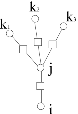
Figure 5: Iteration for $q$-col

Looking to Figure 5, suppose variable $i$ has color $p$ forbidden (i.e. the message $\vec{u}_{a\to i}$ has a $1$ on component $p$). This implies that on this configuration, variable $j$ is forced to take color $p$, that is $\vec{h}_{j\to a}$ is of the form $\left(1,\dots,1,0,1,\dots,1\right)$, with a single $0$ in the $p$-th position (“freezing” type). For all other $h_{j\to a}$ the variable $j$ is in the joker state and the output message will be $\left(0,\dots,0\right)$.

IV.9 Decimation

Once the convergence is reached in Eq. (20) (we stop when $\max_{a\in A,i\in I(a)}\left|{}^{old}Q_{a\to i}-^{new}Q_{a\to i}\right|$ becomes small enough), we can use the information computed so far to find a solution to the original problem MZ_pre ; nosotros . We can easily compute (approximately) the local-field distributions $\left\{H_{i}\right\}_{i\in I}$ introduced in Eq. (13) by considering all neighboring function nodes, and forbidding contradictory messages (remember that in the cavity graph we have deleted the constraints containing variable $i$, whereas in $H_{i}$ we have to restrict the sum to messages being “extensible” to solutions of the complete problem):

$$H_{i}(\vec{h})={\cal Z^{\prime}}^{-1}\sum_{\{\vec{u}_{a\to i}\}_{a\in A(i)}}\left(1-\delta_{\vec{h},(1,...,1)}\right)\ \delta_{\vec{h},\vec{h}_{i}}\prod_{a\in A(i)}Q_{a\to i}(\vec{u}_{a\to i})\ ,$$ (26)

with $\vec{h}_{i}$ determined according to Eq. (IV.3).

The value $H_{i}((1,...,1,0,1,...,1))$, with a single zero entry at component $p$, gives now the probability of a variable $i$ to be frozen to a certain value $p$. A simple decimation procedure can be implemented: Select the most frozen variable and fix it to its most frozen value, then simplify the problem: Certain constraints may already be satisfied independently of the values of other participating variables, and can be deleted from the problem instance. Other constraints may now immediately fix single variables to one state (unit-clause resolution). Reconverge the warning distributions on the smaller subproblem.

The decimation algorithm can have three types of behaviors:

1. The algorithm is able to solve the problem fixing all, or almost all variables (some variables may be still unfixed even if the problem is already solved).

2. The surveys converge at some stage to the trivial solution concentrated on null messages, $Q_{a\to i}(u)=\delta_{h,(0,\dots,0)}$ for all $(i,a)\in E$. In this case SP has nothing more to offer. Luckily, these problems are generally under-constrained and then easy to solve by other means. Note that, for $q$-col, the trivial solution exists always. In numerical experiments, we found that in case of existence of another solution, the latter was the correct one. In this case it is therefore reasonable to restart the iteration of the SP equations starting from a new random initial condition, even if a trivial solution was found once. Only if no non-trivial solution can be found after several restarts, the subproblem is passed to a different solver.

3. The SP algorithm does not converge at some stage, even if the initial problem was satisfiable.

On large random instances of $3$-sat nosotros ; MZ_pre ; MEPAZE ; GP or $q$-col Coloring_algo , in the hard sat region, but not too close to the satisfiability threshold, numerical experiments show that the algorithm behaves as in case 2).

The generated subproblems turn out to be very simple to solve by other conventional heuristics, e.g. walksat walksat or unmodified belief propagation.

Case 3) happens in general very close to the SAT/UNSAT transition. It is not yet clear if this problem appears due to the existence of finite loops in the original problem (which make the SP equations to be only approximate), due to the simple decimation heuristic which fixes always the most frozen variable, or due to some problems which go beyond the validity of the SP equation itself.

V What’s next

We would like to remark two possible directions of research, among all those that may follow from the presented algorithm. One is to formalize rigorously the notions suggested in Section IV, allowing for some well defined definitions of the clusters, and a corresponding derivation of the SP equations.

Another one, of big computational relevance, is to generalize SP, which was presented in its purest form, to deal with correlations between warnings that arise from local problem structures like small loops in the factor graph, cf. YedFreeWei for similar generalizations of BP. A second possible generalization would include diverse structures of the space of solutions, e.g. in a sense of clusters of solution clusters etc. In the language of statistical physics, this would include “more than one step of replica-symmetry breaking”.

After completing this work, we learned from G. Parisi that he has reached a similar conclusion on the interpretation of SP in the colouring problem through the addition of an extra state for the variables GP_white .

Acknowledgment: It is a pleasure to thank R. Mulet, A. Pagnani, and F. Ricci-Tersenghi for numerous discussions. MM and MW acknowledge the hospitality of the ICTP Trieste where a part of this work was done. This work has been supported in part through the EC ’STIPCO’ network, grant No HPRN-CT-2002-00319.

References

- (1) Analytic and algorithmic solutions to random satisfiability problems, M. Mézard, G. Parisi, and R. Zecchina, Science 297, 812 (2002) (Sciencexpress published on-line 27-June-2002; 10.1126/science.1073287).
- (2) Survey propagation: An algorithm for satisfiability, A. Braunstein, M. Mezard, and R. Zecchina, preprint URL: http://lanl.arXiv.org/cs.CC/0212002.
- (3) Random K-satisfiability: from an analytic solution to a new efficient algorithm, M. Mézard and R. Zecchina, Phys.Rev. E 66 056126 (2002).
- (4) Coloring Random Graphs, R. Mulet, A. Pagnani, M. Weigt, and R. Zecchina, Phys. Rev. Lett. 89., 268701 (2002).
- (5) On the survey-propagation equations for the random K-satisfiability problem, G. Parisi, preprint URL: http://lanl.arXiv.org/cs.CC/0212009.
- (6) Factor Graphs and the Sum-Product Algorithm, F.R. Kschischang, B.J. Frey, H.-A. Loeliger, IEEE Trans. Infor. Theory 47, 498 (2002).
- (7) Generalized Belief Propagation J.S. Yedidia, W.T. Freeman and Y. Weiss, in Advances in Neural Information Processing Systems 13 eds. T.K. Leen, T.G. Dietterich, and V. Tresp, pp. 689-695, (Cambridge, MA, MIT Press, 2001).
- (8) Low-Density Parity-Check Codes, R. G. Gallager (Cambridge, MA, MIT Press, 1963).
- (9) Probabilistic Reasoning in Intelligent Systems, J. Pearl, 2nd ed. (San Francisco, Morgan Kaufmann, 1988).
- (10) The cavity method at zero temperature M. Mézard and G. Parisi, J. Stat. Phys. 111, 1 (2003).
- (11) Polynomial iterative algorithms for coloring and analyzing random graphs, A. Braunstein, R. Mulet, A. Pagnani, M. Weigt, and R. Zecchina, Phys. Rev. E 68, 036702 (2003).
- (12) www.ictp.trieste.it/zecchina/SP
- (13) Local search strategies for satisfiability testing , B. Selman, H. Kautz, B. Cohen, in: Proceedings of DIMACS, p. 661 (1993).
- (14) G. Parisi, in preparation.