Stochastic Path Integral Formulation of Full Counting Statistics

Abstract

We derive a stochastic path integral representation of counting statistics in semi-classical systems. The formalism is introduced on the simple case of a single chaotic cavity with two quantum point contacts, and then further generalized to find the propagator for charge distributions with an arbitrary number of counting fields and generalized charges. The counting statistics is given by the saddle point approximation to the path integral, and fluctuations around the saddle point are suppressed in the semi-classical approximation. We use this approach to derive the current cumulants of a chaotic cavity in the hot-electron regime.

Noise properties of electrical conductors are interesting because they reveal additional information beyond linear response BB . In the pioneering work of Levitov and Lesovik Levitov1 , the optics concept of full counting statistics (FCS) for photons was introduced for electrons in the context of mesoscopic physics. FCS gives the probability of counting a certain number of particles at a measurement apparatus in a certain amount of time and finds not only conductance and shot noise, but all higher current cumulants as well. Several methods have been used in finding this quantity. Originally, quantum mechanical methods based on scattering theory Levitov1 ; Muzykantskii1 , the Keldysh approach put forth by Nazarov Nazarov1 or sigma-models Gefen1 have been advanced and have been successfully applied to a number of problems among which we mention only multiterminal structures Bagrets1 , normal-superconducting samples Belzig1 , combined photon/electron statistics Schomerus1 , and conductors which are current (instead of voltage) biased Kindermann1 .

A quantum mechanical treatment of transport shows that the leading contribution to current cumulants is of the order of the channel number $N$. For many conductors or circuits of interest, this leading order is a semi-classical quantity Beenakker1 . Weak localization or universal conductance fluctuations provide only a small correction of order $1$. Clearly, it is desirable to have a purely semi-classical theory to calculate semi-classical results. To provide such a derivation of FCS is the main purpose of this work.

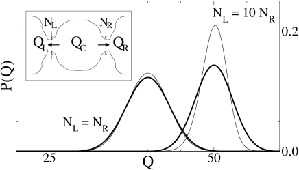
Figure 1: Full counting statistics of a chaotic cavity at zero temperature: Comparison between hot (thick lines) and cold (thin lines) electron regime for both symmetric ($\langle Q\rangle=40e$) and asymmetric ($\langle Q\rangle=50e$) cases. Inset: The chaotic cavity with two point contacts.

That a purely classical theory should be developed was realized by de Jong DeJong1 who put forth a discussion for problems which can be described with the help of master equations. A more general approach, leading to a set of rules for a cascade of higher order cumulants, was recently invented by Nagaev Nagaev1 and applied to chaotic cavities Nagaev2 . The work presented here aims at providing a foundation for the cascade approach by deriving a functional integral from which FCS, but also dynamical quantities such as correlation functions, can be obtained.

The approach provided here applies to an arbitrary mesoscopic network. Its semi-classical nature does not allow the treatment of weak localization corrections nor is it applicable to macroscopic quantum effects like the proximity effect. As in Boltzmann-Langevin theory Kogan1 , our approach is based on a separation of time scales: fast microscopic fluctuations causes variations of conserved quantities (like the charge inside the conductor) on much longer time scales. Whenever such a separation of time scales is present in a stochastic problem, the formalism outlined here is useful. This includes for example normal-diffusive wires Nagaev1 ; Henny , superconducting-normal structures outside the proximity regime Sanquer , as well as stochastic problems beyond mesoscopic physics Langevin .

Path integral derivation. To introduce our path integral formalism, we consider a simple example of electron transport through a chaotic cavity (see Fig. 1) which is a large conductor connected to two metallic leads $L$ and $R$ through ideal point contacts. The leads are at different chemical potentials $\mu_{R}$ and $\mu_{L}=\mu_{R}+eV$, causing a current $I$ to flow through the cavity. The number of modes in each point contact $N_{L,R}$, and the number of states $eVn_{F}$ ($n_{F}$ being a Fermi density of states in the cavity) are large, so that the transport is classical. We assume elastic transport (no energy relaxation), zero temperature, and chaotic electron dynamics in the cavity commentm1 . Then, the state of the cavity is described by only one variable $f_{C}$ which is independent of the electron’s coordinate, momentum and energy in the interval $\mu_{R}<\varepsilon<\mu_{L}$ Langen ; cavity . The average values of outgoing currents $I_{L,R}$ are given by $\langle I_{R}\rangle=(e^{2}V/2\pi\hbar)N_{R}\langle f_{C}\rangle$ and $\langle I_{L}\rangle=-(e^{2}V/2\pi\hbar)N_{L}(1-\langle f_{C}\rangle)$. Since currents are conserved $\langle I_{L}\rangle+\langle I_{R}\rangle=0$, the average current through the cavity is $\langle I\rangle=(e^{2}V/2\pi\hbar)[N_{L}N_{R}/(N_{L}+N_{R})]$, i.e. the resistances of the two point contacts add.

The currents $I_{L,R}$ however fluctuate as a result of the discretness of the electron charge. These fast fluctuations (correlated on the time scale $\tau_{0}\sim\hbar/eV$) cause slow variations of the occupation $f_{C}$ on the scale of the relaxation time $\tau_{C}=2\pi\hbar n_{F}/(N_{L}+N_{R})$ comment0 ; Brouwer . The cause of this is charge conservation: $I_{L}+I_{R}=-\dot{Q}_{C}$, where $Q_{C}=e^{2}n_{F}Vf_{C}$ is the charge accumulated in the cavity. Fluctuations of $f_{C}$ in turn affect the currents $I_{L,R}$ thereby generating correlations between them. Our goal is to integrate out currents $I_{L,R}$ taking into account correlations and to obtain the FCS of the transmitted charge $Q(t)=(1/2)\int^{t}_{0}dt^{\prime}[I_{R}(t^{\prime})-I_{L}(t^{\prime})]$. More precisely, we have to find the generator $S(\chi,t)$ of the charge cumulants defined as

$$P(Q,t) = (2\pi)^{-1}\int d\chi\exp[-i\chi Q+S(\chi,t)],$$ (1)

$$\langle Q^{m}(t)\rangle = \partial^{m}S(\chi,t)/\partial(i\chi)^{m}|_{\chi=0}$$ (2)

where $P(Q,t)$ is the distribution of transmitted charge, and $\langle Q^{m}(t)\rangle$ is its $m$-th cumulant. The average current and its zero-frequency noise power are given respectively by the first cumulant $\langle Q(t)\rangle/t$, and second cumulant $\langle Q^{2}(t)\rangle/t$, after taking the limit $t\to\infty$.

The separation of time scales $\tau_{C}/\tau_{0}\gg 1$ allows us to consider the intermediate time interval $\Delta t$, such that $\tau_{0}\ll\Delta t\ll\tau_{C}$, on which the occupation $f_{C}$ is approximately constant in time. Then the charges transmitted through the point contacts during this time interval, $Q_{L,R}=\int^{\Delta t}_{0}dt^{\prime}I_{L,R}$, are not correlated, i.e. the total distribution is a product $P_{L}(Q_{L})P_{R}(Q_{R})$. On the other hand, since $\Delta t$ is large compared to the correlation time $\tau_{0}$, their distributions $P_{L,R}$ can be written as Fourier integrals (1) with the cumulant generators proportional to time $\Delta t$ comment1 , namely $S_{L,R}=H_{L,R}\Delta t$. They are well known Levitov1 and for ideal point contacts given by

$$H_{L,R} = (N_{L,R}/2\pi\hbar)\int d\varepsilon\left\{\ln[1+f(\varepsilon)(e^{ie\chi_{L,R}}-1)]\right.$$ (3)

$$+ \left.\ln[1+f_{L,R}(\varepsilon)(e^{-ie\chi_{L,R}}-1)]\right\}.$$

For elastic transport, only the energy interval $\mu_{R}<\varepsilon<\mu_{L}$ contributes with $f_{L}=1$, $f_{R}=0$, and $f=f_{C}$.

To proceed with our derivation we first discretize time, $t_{n}=n\Delta t$, $n=1,\ldots,N$, and write the characteristic function of transmitted charge $\exp[S(\chi,t)]$ for the unconditional probability distribution

$$\exp[S(\chi,t)] = \prod_{n}\prod_{l=L,R}\int dQ_{l}(t_{n})P_{l}[Q_{l}(t_{n})]$$ (4)

$$\times \exp\bigg{\{}\frac{i\chi}{2}\sum\limits_{n}[Q_{R}(t_{n})-Q_{L}(t_{n})]\bigg{\}}.$$

Next, we impose a constraint

$$f_{C}(t_{n+1})=f_{C}(t_{n})-(e^{2}n_{F}V)^{-1}[Q_{L}(t_{n})+Q_{R}(t_{n})],$$ (5)

which guarantees the conservation of charge on the cavity, and gives dynamics to the fluctuating charge $Q_{C}$. Integrating out the charges $Q_{L,R}(t_{n})$ in Eq. (4) with the use of Eqs. (1) and (5), and taking a continuum limit, we obtain one of our main results

$$\exp[S(\chi,t)]=(2\pi)^{-1}\int{\cal D}Q_{C}{\cal D}\chi_{C}$$

$$\qquad\times\exp\left\{\int_{0}^{t}dt^{\prime}[i\chi_{C}\dot{Q}_{C}+H(\chi,\chi_{C},Q_{C})]\right\},$$ (6)

where $H(\chi,\chi_{C},Q_{C})$ is

$$H=H_{L}(\chi_{C}-\chi/2,f_{C})+H_{R}(\chi_{C}+\chi/2,f_{C})$$ (7)

with $H_{L,R}$ given by Eq. (3). Eq. (6) resembles the imaginary time path integral for the evolution operator of a quantum particle with coordinate $Q_{C}$, momentum $\chi_{C}$, and Hamiltonian $-H$ with the difference that $H$ given by (7) is not Hermitian. Nevertheless, we can apply the Hamiltonian formalism to our path integral (6). Next, we derive the saddle-point solution and discuss its applicability.

Saddle-point solution. The saddle point of the path integral (6) can be obtained by a variation of the action with respect to $\chi_{C}$ and $Q_{C}$ and gives “classical equations of motion”

$$i\dot{Q}_{C}=-\partial H/\partial\chi_{C},\quad i\dot{\chi}_{C}=\partial H/\partial Q_{C}.$$ (8)

These equations have to be solved with the conditions $Q_{C}=Q_{C}(0)$ for $t^{\prime}=0$, and $\chi_{C}=0$ for $t^{\prime}=t$ comment2 . The solution has to be substituted into Eq. (6) to obtain the saddle-point part $S_{0}$ of the cumulant generator.

Eqs. (8) describe the relaxation of the initial state $Q_{C}(0)$ to the stationary state $\{\bar{\chi}_{C},\bar{Q}_{C}\}$ given by the solution of $\partial H/\partial\chi_{C}=\partial H/\partial Q_{C}=0$. On time scales large compared to the relaxation time $\tau_{C}$, the initial and final integration points contribute little (see discussion below), and we can neglect the first term in the action (6). This gives us a large time asymptotics SP-solution ,

$$S_{0}(\chi,t)=tH(\chi,\bar{\chi}_{C},\bar{Q}_{C}),\quad t\gg\tau_{C},$$ (9)

which will be analyzed below.

To further simplify the analysis, we concentrate on the symmetric cavity with equal number of modes $N_{L}=N_{R}=N_{pc}$ in the contacts. Then the stationary saddle-point solution can be found analytically giving $\bar{\chi}_{C}=0$, $\bar{f}_{C}=1/2$, and

$$S_{0}(\chi,t)=(eVN_{pc}t/\pi\hbar)\ln[(1/2)(1+e^{ie\chi/2})]$$ (10)

which is the known result for a symmetric cavity found from quantum mechanical calculations Blanter .

To investigate the validity of the saddle-point solutions (8) and (9) we calculate the contribution of Gaussian fluctuations by expanding $S$ in the vicinity of the stationary point to second order in $\chi_{C}$ and $Q_{C}$. For the correction to $S_{0}$ we obtain the action of a harmonic oscillator in imaginary time comment3 with inverse frequency $\omega^{-1}=\tau_{C}\cos(e\chi/4)$ and mass $M=(4\pi\hbar/e^{3}VN_{pc})\cos^{2}(e\chi/4)$. In the context of our problem such an action describes the linear dissipative dynamics $\dot{Q}_{C}=-\omega(Q_{C}-\bar{Q}_{C})+\nu(t)$ with the Gaussian Langevin source $\langle\nu(t)\nu(t^{\prime})\rangle=M^{-1}\delta(t-t^{\prime})$ Langevin , which takes the initial state $Q_{C}(0)$ to the stationary state $\bar{Q}_{C}$ after time $t\sim\tau_{C}$. Integrating out $Q_{C}$ we obtain for the total action $S=S_{0}+\delta S_{0}+S_{fl}$, where $\delta S_{0}=-(1/2)M\omega Q_{C}^{2}(0)\tanh(\omega t)$ is the initial condition contribution and $S_{fl}=-(1/2)\ln[\cosh(\omega t)]$ is the fluctuation contribution. Since in general $Q_{C}(0)\lesssim e^{2}n_{F}V$, the part $\delta S_{0}$ is small compared to $S_{0}$ if $t\gg\tau_{C}$. The part $S_{fl}$ is small compared to $S_{0}$ if $en_{F}V\gg 1$, which has been assumed for our classical cavity comment4 . All this justifies the saddle-point solution (9). Having established the framework of our formalism, we now proceed with its generalization and applications.

Generalization. We consider the nonequilibrium dynamics of an arbitrary classical system, which can be described by fast fluctuating currents $I_{\alpha\beta}$ and slow fluctuating charges $Q_{\alpha}$. Metallic reservoirs, such as leads and cavities, can be taken into account by replacing $\alpha\to(\alpha,l)$, where the index $l=1,\ldots,L$ enumerates reservoirs, and $\alpha$ enumerates generalized charges in the reservoirs. These charges $Q_{\alpha}$ are defined as $\dot{Q}_{\alpha}=-\sum_{\beta}I_{\alpha\beta}$. Assuming that the probability distributions of fluctuating currents $I_{\alpha\beta}$ are known, we have to find an evolution of the distribution $\Gamma(Q,t)$ of the set of charges $Q=\{Q_{\alpha}\}$ for a given initial condition $\Gamma(Q,0)$. In other words, one has to find an evolution operator $U(Q,Q^{\prime},t)$ such that $\Gamma(Q,t)=\int dQ^{\prime}U(Q,Q^{\prime},t)\Gamma(Q^{\prime},0)$. We use again the separation of time scales, follow the lines of the derivation of Eq. (6), and obtain the evolution operator $U=\exp[S_{0}(Q,Q^{\prime},t)]$, with $S_{0}$ being a saddle-point solution of the action

$$S=\int_{0}^{t}dt^{\prime}[i\chi\dot{Q}+(1/2)\sum_{\alpha\beta}H_{\alpha\beta}(\chi_{\alpha}-\chi_{\beta})],$$ (11)

where $\chi=\{\chi_{\alpha}\}$ is the set of charge counting fields. The generators $H_{\alpha\beta}$ of the cumulants of currents $I_{\alpha\beta}$ have the obvious symmetry $H_{\alpha\beta}(\chi_{\alpha}-\chi_{\beta})=H_{\beta\alpha}(\chi_{\beta}-\chi_{\alpha})$.

Next we assume that the “Hamiltonian” $H=(1/2)\sum_{\alpha\beta}H_{\alpha\beta}$ depends only on the subset of charges $Q^{c}=\{Q^{c}_{\alpha}\}$, which we call conserved charges since they are related to conserved quantities, such as total energy and charge. We complete the set $Q=\{Q^{c},Q^{a}\}$ by the subset of non-conserved or absorbed charges $Q^{a}=\{Q^{a}_{\alpha}\}$. Since $H$ does not depend on $Q^{a}$, we find that the corresponding “momentums” $\chi^{a}=\{\chi^{a}_{\alpha}\}$ are integrals of motion: $\chi^{a}=const$. This allows us to integrate out the corresponding terms in (11): $i\int_{0}^{t}dt^{\prime}\chi^{a}\dot{Q}^{a}=i\chi^{a}[Q^{a}(t)-Q^{a}(0)]$. Thus the rest of the action (11) becomes a generator of cumulants of the absorbed charge $Q^{a}(t)-Q^{a}(0)$. In particular, the stationary solution for the cumulant generator is $S_{0}=tH(\chi^{a},\bar{\chi}^{c},\bar{Q}^{c})$, where $\bar{\chi}^{c}$ and $\bar{Q}^{c}$ are solutions of the equations $\partial H/\partial\chi^{c}=\partial H/\partial Q^{c}=0$.

In the example of the elastic transport considered above there are 3 reservoirs: Two leads ($\alpha=1,3$) and one cavity ($\alpha=2$). The state of the cavity is described by only one charge $Q_{C}=Q_{2}$, the total charge on the cavity, while $Q=(Q_{3}-Q_{1})/2$ is the absorbed charge which is being counted. The counting fields are $\chi_{C}=\chi_{2}$, and $\chi/2=\chi_{1}=-\chi_{3}$. Next we consider the case of inelastic transport, which requires the introduction of a new generalized conserved charge $E_{C}$, the total energy of the cavity.

Hot-electron regime. We consider the electron transport through a cavity in the so-called hot-electron regime, i.e. when the electron-electron scattering time is much shorter than the relaxation time $\tau_{ee}\ll\tau_{C}$, electrons in the cavity then relax to local thermal equilibrium before escaping from the cavity. Their distribution is given by a Fermi function $f(\varepsilon)=\{1+\exp[(\varepsilon-\mu_{C})/T_{C}]\}^{-1}$ where $\mu_{C}$ and $T_{C}$ denote respectively the electro-chemical potential and electron temperature in the cavity. The noise in the hot-electron regime was first considered theoretically for diffusive wires Rudin1 . This calculation and its experimental verification Henny1 found that electron-electron interaction increases shot noise. Similar results for the chaotic cavity were presented in Ref. Beenakker1 and measured in Ref. Oberholzer1 . We now derive the FCS of transmitted charge $Q$.

Our calculation starts from the observation that the nonequilibrium state of the cavity is fully described by only two parameters, $\mu_{C}$ and $T_{C}$. They can be expressed in terms of conserved values: The total charge $Q_{C}=e^{-1}C_{\mu}\mu_{C}$ and the total energy $E_{C}=(1/2C_{\mu})Q_{C}^{2}+Q_{C}V_{G}+(\pi^{2}/6)n_{F}T_{C}^{2}$ of the cavity, where $C_{\mu}$ is the electrochemical capacitance of the cavity, $1/C_{\mu}=1/C+1/(e^{2}n_{F})$, and $V_{G}$ is the gate voltage. The charge and energy conservation can be written as

$$\int d\varepsilon\,[I_{L}(\varepsilon)+I_{R}(\varepsilon)]=-\dot{Q}_{C},$$ (12)

$$\int d\varepsilon\,\varepsilon\,[I_{L}(\varepsilon)+I_{R}(\varepsilon)]=-e\dot{E}_{C},$$ (13)

where $I_{L,R}(\varepsilon)$ are the outgoing currents through the point contacts per energy interval $d\varepsilon$. We now replace the constraint (5) with these two equations, and apply it to the energy resolved analogue of path integral (4). By doing so, we introduce the counting field $\chi_{E}$ for the total energy $E_{C}$. Instead of (7), the new “Hamiltonian” $H(\chi,\chi_{C},\chi_{E};\mu_{C},T_{C})$ takes the form

$$H=\int d\varepsilon[H_{L}(\chi_{C}+\varepsilon\chi_{E}-\chi/2)+H_{R}(\chi_{C}+\varepsilon\chi_{E}+\chi/2)],$$ (14)

with $H_{L,R}$ given by Eq. (3).

To obtain the FCS in the long time limit $t\gg\tau_{C}$, where $\tau_{C}=2\pi\hbar C_{\mu}/[e^{2}(N_{L}+N_{R})]$ is the RC-time (the time of charge screening in the cavity Brouwer ), we need to evaluate $H$ as a function of $\chi$ at the saddle point. We find the saddle-point solution $S_{0}(\chi,t)$ numerically and calculate $P(Q,t)$ by Fourier transformation (1). The result is shown in Fig. 1. It is clearly visible that noise is enhanced in the hot-electron regime.

In order to make further analytical progress we note that the saddle point solution for $\chi=0$ is given by the chemical potential $\mu_{C}=(N_{L}\mu_{L}+N_{R}\mu_{R})/(N_{L}+N_{R})$ and the effective temperature $T_{C}=\sqrt{T^{2}+T^{2}_{V}}$, where $T$ is the temperature of the reservoirs, and $T_{V}=(\sqrt{3}/\pi)\eta eV$ is proportional to bias with $\eta^{2}=N_{L}N_{R}/(N_{L}+N_{R})^{2}$. The internal fields $\chi_{C},\chi_{E}$ are zero for $\chi=0$. It is now straightforward to expand Eq. (14) and the corresponding saddle point equations around $\chi=0$ and to calculate higher cumulants order by order. This procedure is very similar to the cascade approach considered in Refs. Nagaev1 ; Nagaev2 . For the first few cumulants we obtain

$$\langle Q^{2}\rangle = \frac{e^{2}\eta t}{2\pi\hbar}\sqrt{N_{L}N_{R}}\;\left(T+T_{C}\right),$$ (15a)

$$\langle Q^{3}\rangle = -\frac{e^{3}\eta^{2}t}{2\pi\hbar}\sqrt{N_{L}N_{R}}\;\frac{3\sqrt{3}TT_{V}}{\pi T_{C}}\,,$$ (15b)

$$\langle Q^{4}\rangle = \frac{e^{4}\eta^{3}t}{2\pi\hbar}\sqrt{N_{L}N_{R}}\frac{9}{\pi^{2}}\left[T-T_{C}+\frac{2T^{4}}{T_{C}^{3}}\right],$$ (15c)

where the second cumulant coincides with the one in the Ref. Oberholzer1 . The result for the third cumulant shows that odd cumulants are strongly suppressed. We note that screening does not affect the FCS in the long time limit $t\gg\tau_{C}$.

Conclusions. We have constructed a stochastic path integral formulation of full counting statistics. Our approach is based on the fact that fast microscopic quantum fluctuations give rise to slow variations of conserved quantities. The method has been illustrated with chaotic cavities and novel results have been presented for the hot-electron regime. We emphasize the general nature of this approach and its applicability to stochastic problems even outside mesoscopic physics.

S. P. acknowledges the collaboration with K. E. Nagaev on an earlier related work. We thank P. Samuelsson for useful discussions. This work was supported by the Swiss National Science Foundation.

References

- (1) Ya. M. Blanter and M. Büttiker, Physics Reports 336, 1-166 (2000).
- (2) L. S. Levitov and G. B. Lesovik, Pis’ma Zh. Eksp. Teor. Fiz. 58, 225 (1993).
- (3) B. A. Muzykantskii and D. E. Khmelnitskii, Phys. Rev. B 50, 3982 (1994).
- (4) Yu. V. Nazarov, Ann. Phys. (Leipzig) 8 Spec. Issue, S1-193 (1999).
-
(5)
D.G. Gutman, Yuval Gefen, A.D. Mirlin,
cond-mat/0210076. - (6) Yu. V. Nazarov and D. A. Bagrets, Phys. Rev. Lett. 88, 196801 (2002); F. Taddei and R. Fazio, Phys. Rev. B 65, 075317 (2002).
- (7) W. Belzig and Yu. V. Nazarov, Phys. Rev. Lett. 87, 197006 (2001); P. Samuelsson and M. Büttiker, Phys. Rev. B 66, 201306 (2002).
- (8) C. W. J. Beenakker and H. Schomerus, Phys. Rev Lett. 86, 700 (2001).
- (9) M. Kindermann, Yu. V. Nazarov, and C. W. J. Beenakker, cond-mat/0210617.
- (10) M. J. M. de Jong and C. W. J. Beenakker in Mesoscopic Electron Transport, L. P. Kouwenhoven, G. Schön, L. L. Sohn eds., NATO ASI Series E, Vol. 345 (Kluwer Academic, Dordrecht 1996).
- (11) M. J. M. de Jong, Phys. Rev. B 54, 8144 (1996).
- (12) K. E. Nagaev, Phys. Rev. B 66, 075334 (2002).
- (13) K. E. Nagaev, P. Samuelsson, and S. Pilgram, Phys. Rev. B 66, 195318 (2002).
- (14) Sh. M. Kogan and A. Ya. Shul’man, Zh. Eksp. Teor. Fiz. 56, 862 (1969).
- (15) M. Henny et al., Phys. Rev. B 59, 2871 (1999).
- (16) X. Jehl, and M. Sanquer, Phys. Rev. B 63, 052511 (2001).
- (17) J. Zinn-Justin, Quantum field theory and critical phenomena, Clarendon Press (Oxford, 1993).
- (18) We assume that the flight times through the contacts and cavity are the shortest time scales.
- (19) S. A. van Langen, and M. Büttiker, Phys. Rev. B 56, 1680 (1997).
- (20) Ya. M. Blanter, and E. V. Sukhorukov, Phys. Rev. Lett. 84, 1280 (2000).
- (21) In this example is the dwell time, while for the case of screening considered later it becomes an RC relaxation time, see Ref. Brouwer .
- (22) P. W. Brouwer, and M. Büttiker, Europhys. Lett. 37, 441 (1997).
- (23) The currents are Markovian on the time scale , implying the semigroup property , .
- (24) The integration in (6) goes over the whole set of variables except the initial condition . According to Eq. (5) does not depend on . Thus the integration over in (6) fixes the condition .
- (25) A similar result was found in Ref. Kindermann1 using a fully microscopic theory based on Keldysh technique.
- (26) Ya. M. Blanter, H. Schomerus, C. W. J. Beenakker Physica E 11, 1 (2001).
- (27) This is true up to a boundary term .
- (28) The contribution depends on the approximate time discretization procedure (5), and thus the numerical prefactor in is beyond our formalism (this is related to the usual operator ordering ambiguities in path integrals Langevin ). Fortunately, as we have shown, is small and can be neglected compared .
- (29) K. E. Nagaev, Phys. Rev. B 52, 4740 (1995); V. I. Kozub and A. M. Rudin, Phys. Rev. B 52, 7853 (1995).
- (30) A. H. Steinbach, J. M. Martinis, and M. H. Devoret, Phys. Rev. Lett. 76, 3806 (1996); M. Henny et al., Phys. Rev. B 59, 2871 (1999).
- (31) S. Oberholzer et al., Phys. Rev. Lett. 86, 2114 (2001).