Glass transition as a decoupling-coupling mechanism of rotations

Abstract

We introduce a three-dimensional lattice gas model to study the glass transition. In this model the interactions come from the excluded volume and particles have five arms with an asymmetrical shape, which results in geometric frustration that inhibits full packing. Each particle has two degrees of freedom, the position and the orientation of the particle. We find a second order phase transition at a density $\rho\approx 0.305$, this transition decouples the orientation of the particles which can rotate without interaction in this degree of freedom until $\rho=0.5$ is reached. Both the inverse diffusivity and the relaxation time follow a power law behavior for densities $\rho\leq 0.5$. The crystallization at $\rho=0.5$ is avoided because frustration lets to the system to reach higher densities, then the divergencies are overcome. For $\rho>0.5$ the orientations of the particles are coupled and the dynamics is governed by both degrees of freedom.

I Introduction

In the last years, a great deal of work has been done to obtain a fundamental understanding of the glass transition. Many questions about the equilibrium and the dynamical properties of the glassy state remain ananswered. It is not clear if there is a true phase transition and what is the role that geometric frustration plays on it. The relations between the equilibrium and the dynamical properties are not understood M01 . The mode coupling theory for supercooled liquids G91 predicts the existence of a temperature $T_{\rm c}$ at which there is a crossover from a liquid to a glassy state. In the glassy state the dynamics would be dominated by complex activated processes. For temperatures $T>T_{\rm c}$ but close to $T_{\rm c}$ there is a power law behavior of the relaxation time and also of the inverse diffusivity. It is not understood whether $T_{\rm c}$ is a purely kinetic transition temperature G91 or if it is a true thermodynamic glass transition which is kinetically avoided DS01 . Several lattice gas models have been used to simulate glassy systems and have reproduced some aspects of the glassy phenomenology. For example the Hard Square Model (HSM) GF66 , the Kinetically Constrained Model FA84 ; GP97 , the Frustrated Ising Lattice Gas Model NC98 , the one introduced by Ciamarra et al. C02 , and recently the Lattice Glass Model (LGM) BM01 . The LGM model with density constraint $l=0$ is equivalent to the the three-dimensional HSM model also called Hard Cubic Model (HCM). The LGM model relates the glass transition to a first order phase transition.

In this paper we consider a three-dimensional lattice gas model, which contains as main ingredients only geometric frustration without quenched disorder and without kinetic or density constraints, as quenched disorder is not appropriate to study structural glasses and kinetic or density constraints are some how artificial. Similar models have already been proposed and studied in two-dimensional systems C94 ; BK01 ; DD02 and applied to study granular material CL97 .

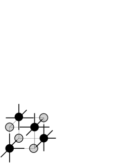
Figure 1: Schematic picture of one particular configuration in a system size of $N=2^{3}$ and density $\rho=0.5$. Shadow spheres represent holes in the system. Black spheres are particles with five arms each one.

II The model

Our model is a generalization to three dimensions of the two-dimensional model studied in Ref. DD02 . It can be considered as an illustration of the concept of frustration arising as a packing problem. We have particles with five arms and they occupy the vertices of a cubic lattice with one of six possible orientations. Assuming that the arms cannot overlap due to excluded volume, we see that only for some relative orientations two particles can occupy nearest-neighbor vertices. Consequently, depending on the local arrangement of particles, there are sites on the lattice that cannot be occupied (see Fig. 1). This type of “packing” frustration thus induces defects or holes in the system. We impose periodic boundary conditions in the cubic lattice of size $N=L^{3}$. The maximum of density is $\rho_{\rm max}=3/5$ at which all possible bonds are occupied by an arm. Here we have two degrees of freedom for each particle, the position and the orientation of the particle. This model is the HCM model when the particles have six instead five arms. Our model would be also similar to the LGM model with the density constraint $l=1$. We will compare the results found in our model with the ones obtained in these two models. We have used two algorithms in order to make the simulations. The first one (CA) is the Monte Carlo simulation at fixed density in the canonical ensemble, we have simulated the diffusion and rotation dynamics of the particles by the following algorithm: i) Pick up a particle at random; ii) Pick up a site at random between the six nearest neighbor ones; iii) Choose randomly an orientation of the particle; iv) If it does not cause the overlapping of two arms, move the particle in the given site with the given orientation; v) If the diffusion movement is not possible, choose a random orientation and try to rotate the particle to this new orientation; vii) Advance the clock by $1/N$, where $N$ is the number of sites, and go to i). The second algorithm (GCA) is the grand canonical ensemble, the diffusion and rotation dynamics is as in the CA simulations but now a reservoir with chemical potential $\mu$ is coupled to each lattice site which can create (if it does not cause the overlapping of two arms) or destroy particles. As we expect the GCA simulation reaches the equilibrium faster. We will use the GCA simulation in order to find the behavior of the density $\rho$ with $\mu$ BM01 .

III Results

We first study a possible first order phase transition in our model. In the inset of Fig. 2 the inverse of the density is plotted as a function of the chemical potential. As in Ref. BM01 we make GCA simulations to obtain this figure. A maximum of density very close to $\rho_{\rm max}$ is reached without any discontinuity, although we observe finite-size effects which prevent to reach $\rho_{\rm max}$ for the lattice sizes studied here. So, first order phase transition is not present in our system. In the HCM model we also observe similar behavior of the density with $\mu$ reaching the maximum of density continously, $\rho_{\rm max}=0.5$ in the HCM model. Instead, in the LGM model with $l\geq 1$ there is always a first order phase transition BM01 .

We now calculate the diffusion coefficient $D$ from the mean-square displacement of the particles at very long times with the CA simulations. The values obtained for $D$ are well fitted by a power law close to $\rho_{\rm c}=0.52\pm 0.005$ and for densities lower than $\rho=0.5$, $D\propto(\rho_{\rm c}-\rho)^{\gamma}$ with $\gamma=2.45\pm 0.01$ (see Fig. 2). This anomalous behavior of $D$ near of $\rho_{\rm c}$ would indicate a crossover density, from liquid to glass phase, where activated processes dominate in the glass phase. As it happens in the HSM model F89 the finite size effects for the diffusivity in the HCM model are very large when we do CA simulations, it is because the particles can be enclosed in cages and the diffusion is blocked. It prevents to reach densities close to the maximum density. Nevertheless, in our model the finite size effects are only important for $\rho>0.58$ when $N=14^{3}$. This is because our model has two degrees of freedom and rotations prevent to find blocked configurations for $\rho<0.58$.

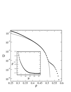
Figure 2: Diffusion constant $D$ as a function of density $\rho$ for a system size of $N=14^{3}$. The fitting function is a power law $D=2.11(0.523-\rho)^{2.45}$. Inset: The inverse of the density as function of $\mu$ on a lattice of size $N=14^{3}$. The data are obtained from the GCA with 2$\times 10^{7}$ Monte Carlo Steps per Particle at a fixed increasing rate of the chemical potential between $\mu=0$ and $\mu=27$.

In order to understand what happens at $\rho\approx 0.5$ we study the following microscopic order parameter. As in anti-ferromagnetic systems, the cubic lattice is divided into two interpenetrating sublattices ($A$ and $B$), a site in a sublattice has six nearest neighbor sites which belong to the other sublattice. The order parameter is defined as

$$\phi=\frac{\rho_{A}-\rho_{B}}{\rho_{A}+\rho_{B}}\,,$$ (1)

where $\rho_{A}$ and $\rho_{B}$ are the equilibrium concentrations of the particles in the sublattices $A$ and $B$ and we have $\rho=\rho_{A}+\rho_{B}$. This parameter can be used to study concentration sublattice ordering. When the particles prefer to stay in one of these sublattices then $\phi\neq 0$. In the left inset of Fig. 3 we show $\phi$ as a function of the density. We can see that it is different to zero for $\rho>\rho_{\rm f}\approx 0.3$ and it increases until $\rho\approx 0.5$, then there is a maximum. For higher densities it decreases linearly with the density. In Fig. 3 we show the concentration in both sublattices. We see that at $\rho_{\rm f}$ the concentrations $\rho_{A}$ and $\rho_{B}$ begin to be different each other, the particles prefer to stay in a sublattice. The concentration in the sublattice $A$ has the maximum value when $\rho=0.5$ is reached. A sublattice is full of particles at this concentration while the other one is in practice empty. The particles begin to occupy the empty sublattice for densities higher than $\rho=0.5$ remaining the other sublattice full, then the parameter $\phi$ decreases. Here we observe that there are not frozen particles at these densities, $\rho_{A}$ and $\rho_{B}$ are equilibrium concentrations. The order parameter $\phi$ can take positive and negative values, it depends on which sublattice has higher density for $\rho>\rho_{\rm f}$, in Fig. 3 we have $\phi>0$ for $\rho>\rho_{\rm f}$ because $\rho_{A}>\rho_{B}$. Similar behavior for the parameter $\phi$ is found in the HCM model but $\rho_{\rm f}\approx 0.22$ is lower than the one obtained in our model and the system crystallizes at $\rho=0.5$, its maximum of density, then the particles are frozen in a sublattice and it is not possible to reach higher densities. So, the last part of Fig. 3 (for $\rho>0.5$) is not found in the HCM model. As we will see below at $\rho_{\rm f}$ there is a continuous phase transition in our model and also in the HCM model. In the LGM model with $l=1$, we have found a first order phase transition with a discontinuity of the density, when is plotted as a function of $\mu$, from a density $\rho\approx 0.32$ to a density $\rho=0.5$, then the system crystallizes and the particles are frozen in a sublattice.

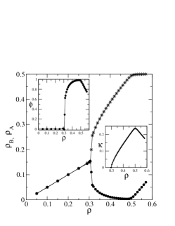
Figure 3: Concentration of particles in sublattices $A$, $\rho_{A}$ (asterisks), and $B$, $\rho_{B}$ (solid circles), as a function of the density $\rho$ for a system size of $L=14$. Left inset: Order parameter $\phi$ as a function of the density $\rho$. Right inset: Compressibility $\kappa$ as a function of the density $\rho$.

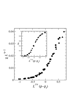
Figure 4: Finite size scaling of $\chi$ and $g$ (inset) for lattice sizes $L=8$ ($\bullet$), 10 ($\blacksquare$), 12 ($\blacklozenge$), 14 ($\blacktriangle$), and 16 ($\blacktriangleleft$). $\rho_{\rm f}=0.305\pm 0.005$, $\eta=0.04\pm 0.01$, and $\nu=0.63\pm 0.05$.

We now study the equilibrium second order phase transition in our system. For that, we define the compressibility by the following expression

$$\kappa=\frac{1}{N}\sum_{i}\left(\langle n_{i}^{2}\rangle-\langle n_{i}\rangle^{2}\right)\,,$$ (2)

where $n_{i}=0,1$ is the occupation number of site $i$ and $\langle\cdots\rangle$ indicates equilibrium average. In the right inset of Fig. 3 we see the behavior of $\kappa$ with the density. We find that the compressibility is different to zero for densities higher than $\rho_{\rm f}\approx 0.305$ and it has a maximum at $\rho=0.5$, decreasing for higher densities. This behavior is similar to the one found for the parameter $\phi$. The associated susceptibility $\chi$ is given by $\chi=N\left(\langle\kappa^{2}\rangle-\langle\kappa\rangle^{2}\right)$ and the Binder’s cumulant is $g=(3-\langle\kappa^{4}\rangle/\langle\kappa^{2}\rangle^{2})/2$. Around a continuous phase transition $\chi$ and $g$ should obey the finite-size scaling $\chi(\rho)=L^{2-\eta}\widetilde{\chi}\left[L^{1/\nu}(\rho-\rho_{\rm f})\right]$ and $g(\rho)=\widetilde{g}\left[L^{1/\nu}(\rho-\rho_{\rm f})\right]$ where $\widetilde{\chi}\left[x\right]$ and $\widetilde{g}\left[x\right]$ are universal functions and $\rho_{\rm f}$ is the critical density. From the finite size scaling (see Fig. 4) we find a continuous phase transition at $\rho_{\rm f}=0.305\pm 0.005$ which belongs to the three-dimensional Ising universality class, $\eta=0.04\pm 0.01$ and $\nu=0.63\pm 0.05$. In the HCM model we have found a second order phase transition which also belong to the same universality class but with $\rho_{\rm f}\approx 0.22$. In Fig. 2 we can see that the diffusion constant is not affected by the second order phase transition.

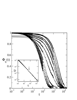
Figure 5: Correlation functions of the density fluctuations $\Phi_{\bf q}(t)$ for ${\bf q}=(\pi/3,\pi/3,\pi/3)$, system size $L=14$, and densities (from bottom to top) $\rho=0.45$, 0.46, 0.47, 0.48, 0.49, 0.5, 0.505, 0.51, 0.515, 0.52, 0.53, and 0.54. The solid lines are fitting functions corresponding to stretched exponential functions. For $\rho\geq 0.515$ we have $\beta=0.94\pm 0.01$. Inset: $D$ as a function of the relaxation time $\tau$. The arrow shows the density $\rho=0.5$. The solid line is the fitting function $D=0.135/\tau$.

We now study the relaxation of the autocorrelation functions of the density fluctuations

$$\Phi_{\bf q}(t)=\frac{\langle\rho_{\bf q}^{*}(t^{\prime}+t)\rho_{{\bf q}}(t^{\prime})\rangle}{\langle|\rho_{\bf q}|^{2}\rangle}\,,$$ (3)

where $\langle\cdots\rangle$ denotes average over the reference time $t^{\prime}$ and $\rho_{\bf q}$ is the Fourier transform on the lattice of the density

$$\rho_{\bf q}(t)=\frac{1}{N}\sum_{i=1}^{n}e^{-i{\bf q}.{\bf r}_{i}(t)}\,,$$ (4)

where ${\bf r}_{i}(t)$ is the position of the $i$th particle at time $t$, $n$ is the number of particles and ${\bf q}$ is the wave number. Because of the periodic conditions on the cubic lattice ${\bf q}=(2\pi/L)(n_{x},n_{y},n_{z})$, with $n_{x},n_{y},n_{z}=1,\ \cdots,\ L/2$. Fig. 5 shows $\Phi_{\bf q}(t)$ for ${\bf q}=(\pi/3,\pi/3,\pi/3)$ and different densities. We can see a two-step relaxation decay for $\rho>0.5$, the second relaxation step can be fitted by a stretched exponential form, $f(t)=f_{0}\exp\left[(t/\tau)^{\beta}\right]$ where the exponent $\beta=0.94\pm 0.01$ remains constant with $\rho$ for $\rho\geq 0.515$. For $\rho<0.49$ we only have a one-step relaxation decay. The relaxation time $\tau$ can be obtained from $\Phi_{\bf q}(t)$. We find that it is proportional to the inverse of the diffusivity, $\tau\propto D^{-1}$, for the whole range of densities studied here (see inset of Fig 5). Thus, the relaxation time follows a power law at $\rho<\rho_{\rm c}$ with the same exponent than the one obtained in the power law of $D^{-1}$ (see Fig. 2).

We now present the results for the self-part of the autocorrelation function of the density fluctuations, defined as

$$\Phi_{\bf q}^{s}(t)=\frac{1}{N\rho}\sum_{i}\langle e^{i{\bf q}({\bf r}_{i}(t^{\prime}+t)-{\bf r}_{i}(t^{\prime}))}\rangle,$$ (5)

where $\langle\cdots\rangle$ denotes average over the reference time $t^{\prime}$. Fig. 6 shows $\Phi_{\bf q}^{s}(t)$ corresponding to ${\bf q}=(\pi,0,0)$ for densities $\rho=0.35$, 0.45, 0.5, and 0.53. For the whole range of densities studied here we find that the whole time interval of $\Phi_{\bf q}^{s}(t)$ can be fitted by a stretched exponential function where the exponent $\beta$ depends on the density. In the inset of Fig. 6 we show $\beta$ as a function of the density. The exponent $\beta$ decreases with the density until a density near $\rho_{\rm f}$ is reached. Starting from this density, which corresponds to the second order phase transition, the exponent increases until $\rho=0.5$ is reached. For $\rho>\rho_{\rm c}$ it becomes constant (within the error bars) $\beta\approx 0.93$. The relaxation time obtained from the fit of $\Phi_{\bf q}^{s}(t)$ is proportional to the inverse of the diffusivity.

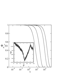
Figure 6: Self-part $\Phi_{\bf q}^{s}(t)$ of the density-density autocorrelations for ${\bf q}=(\pi,0,0)$ and densities $\rho=0.35$, 0.45, 0.5, and 0.53. Dotted lines are fitting functions corresponding to stretched exponential functions. Inset: Parameter $\beta$ of the stretched exponential function for $\Phi_{\bf q}^{s}(t)$ as a function of the density (for each density we plot the error bar of $\beta$).

In order to study the role of the orientation of the particles we define a self-overlap parameter similar to that defined in DF99 for liquids but which also takes into account the orientation of the particles, besides their position. The orientation of a particle is defined by the discrete values of the two orthogonal angles $\theta_{i}=0,\ \pi/2,\ \pi$, or $3\pi/2$ and $\varphi_{i}=0,\ \pi/2,\ \pi$, or $3\pi/2$. We define the self-overlap as

$$q(t)=\frac{1}{N\rho}\sum_{i}^{n}\langle n_{i}(t^{\prime})n_{i}(t^{\prime}+t)$$

$$\cos\left[\theta_{i}(t^{\prime}+t)-\theta_{i}(t^{\prime})\right]\cos\left[\varphi_{i}(t^{\prime}+t)-\varphi_{i}(t^{\prime})\right]\rangle\,,$$ (6)

here $\langle\cdots\rangle$ denotes average over the reference time $t^{\prime}$. If all the particles have the position and the orientation frozen then $q(t)=1$. Fig. 7 shows the parameter $q(t)$ for different values of the density. The plateau becomes visible for densities higher than $\rho\approx 0.5$. From this density there are an important number of particles which have frozen the position and the orientation for a long time. The number of frozen particles and the time during they are frozen increase with the density. We can fit the second relaxation step with the stretched exponential function, but now the exponent $\beta$ decreases with the density from $\beta=0.94$ for $\rho=0.52$ until $\beta=0.77$ for $\rho=0.58$.

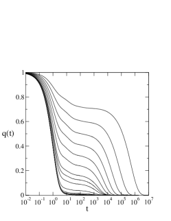
Figure 7: Relaxation functions of the self-overlap $q(t)$ for system size $L=14$ and densities (from bottom to top) $\rho=0.45$, 0.46, 0.47, 0.48, 0.49, 0.5, 0.51, 0.515, 0.52, 0.53, 0.54, 0.55, 0.56, 0.57, and 0.58.

IV Conclusion

We have proposed a three-dimensional lattice gas model, based on the concept of geometric frustration which is generated by the particle shape. In this model a second order phase transition decouples the orientation of the particles which can rotate without interaction in the orientation degree of freedom until $\rho=0.5$ is reached. This is because in practice the particles remain all the time in a sublattice and then the particles can rotate freely. For densities higher than $\rho=0.5$ geometric frustration begins to work and rotations are governed by complex collective processes. Then, the two degrees of freedom are important in the diffusivity movement of the particles. For $\rho\leq 0.5$ the system is going to a crystalline state with all the particles frozen in a sublattice, this brings to a power law divergency of the relaxation time and the inverse of diffusivity for $\rho<0.5$. But frustration lets to the system reach higher densities and crystallization is avoided and the divergencies are overcome. Then, vibrational effects are observed which bring to the two-step relaxation decay in the density correlations and in the self-overlap parameter. Thus, the glass transition is purely a kinetic transition in our model. Geometric frustration plays a fundamental role, without frustration the arrest would be close to $\rho_{\rm c}$, but also the second order phase transition is very important, which decouples the orientation of the particles. In the two-dimensional model DD02 , which has not second order phase transition, we do not observe these anomalies in the diffusivity and relaxation time. The order parameters $\phi$ and $\kappa$ exhibit a maximum at the glass transition $\rho\approx 0.5$.

We have found that the diffusion constant is not affected by the second order phase transition. The self-part of the autocorrelation function of the density fluctuation can be fitted by a stretched exponential function with an exponent $\beta$ that has a minimum value at the second order phase transition and a local maximum at the glass transition.

- (1) M. Mézard, Physica A 306 25 (2002), preprint cond-mat/0110363.
- (2) W. Götze, in Liquids, Freezing and Glass Transition, edited by J.P. Hansen, D. Levesque, and P. Zinn-Justin (Elsevier, Amsterdam, 1991).
- (3) P.G. De Benedetti and F.H. Stillinger, Nature (London) 410, 267 (2001); J.P. Sethna, J.D. Shore, and M. Huang, Phys. Rev. B 44, 4943 (1991).
- (4) D.S. Gaunt and M.E. Fisher, J. Chem. Phys. 45, 2482 (1966); W. Ertel, K. Froböse, and J. Jäckle, J. Chem. Phys. 88, 5027 (1988).
- (5) G.H. Fredrickson and H.C. Andersen, Phys. Rev. Lett. 53, 1244 (1984); J. Chem. Phys. 83, 5822 (1985); W. Kob and H.C. Andersen, Phys. Rev. E 48, 4364 (1993).
- (6) I.S. Graham, L. Piché, and M. Grant, Phys. Rev. E 55, 2132 (1997).
- (7) M. Nicodemi and A. Coniglio, Phys. Rev. E 57, R39 (1998).
- (8) M. Pica Ciamarra, M. Tarzia, A. de Candia, and A. Coniglio, preprint cond-mat/0210144.
- (9) G. Biroli and M. Mézard, Phys. Rev. Lett. 88, 025501-1 (2002).
- (10) A. Coniglio, Nuovo Cimento D 16, 1027 (1994); A. Coniglio Proceedings of the international School of Physics “Enrico Fermi” (Course CXXXIV) (IOS Press, Amsterdam, 1997).
- (11) A. Barrat, J. Kurchan, V. Loreto, and M. Sellitto, Phys. Rev. E 63, 51301 (2001).
- (12) A. Díaz-Sánchez, A. de Candia, and A. Coniglio, J. Phys. A: Math. Gen. 35, 3359 (2002).
- (13) E. Caglioti, V. Loreto, H.J. Herrmann, and M. Nicodemi, Phys. Rev. Lett. 79, 1575 (1997).
- (14) K. Froböse, J. Stat. Phys. 55, 1285 (1989); J. Jäckle, K. Froböse, and D. Knödler, J. Stat. Phys. 63, 249 (1991).
- (15) C. Donati, S. Franz, G. Parisi, and S.C. Glotzer, preprint cond-mat/9905433.