An interacting spin flip model for one-dimensional proton conduction
Abstract
A discrete asymmetric exclusion process (ASEP) is developed to model proton conduction along one-dimensional water wires. Each lattice site represents a water molecule that can be in only one of three states; protonated, left-pointing, and right-pointing. Only a right(left)-pointing water can accept a proton from its left(right). Results of asymptotic mean field analysis and Monte-Carlo simulations for the three-species, open boundary exclusion model are presented and compared. The mean field results for the steady-state proton current suggest a number of regimes analogous to the low and maximal current phases found in the single species ASEP [B. Derrida, Physics Reports, 301, 65-83, (1998)]. We find that the mean field results are accurate (compared with lattice Monte-Carlo simulations) only in the certain regimes. Refinements and extensions including more elaborate forces and pore defects are also discussed.
pacs:
02.50.Ey, 05.70.Ln, 05.50.+q1 Introduction
One-dimensional nonequilibrium processes have been used as models for many systems including interface growth [1, 2], traffic flow [3, 4], pore transport [5, 6, 7], and quantum spin chains [8]. The simple asymmetric exclusion process (ASEP) has also been used to model mRNA translation [9, 10] and recent modifications have been applied in order to describe molecular motors and parallel pathways [11, 12, 13].
Building upon the exact and asymptotic results of Derrida, Evans, Rittenberg, Sandow, and others [8, 14, 15, 16, 17, 18], the quantitative behavior of other more complex one-dimensional systems can be investigated. Asymmetric exclusion processes of multiple species have also been modelled, particularly for periodic boundary conditions [19, 20], or in the context of spontaneous symmetry breaking for open systems [21]. In the proton conduction problem, only one species (protons) are transported while the other classes of particles correspond to different orientation states of the relatively fixed water molecules.
In this paper, we present a restricted three-species exclusion process that models proton conduction through a “water wire.” Our model is motivated by experiments on proton conduction through stable or transient water filaments suggesting conduction occurs via proton exchange between properly aligned water molecules [22, 23]. This “Grotthuss [24]” mechanism of proton conduction along a relatively static water chain has been proposed to give rise to the fast proton transfer rates relative to the permeation of distinguishable ions across structurally similar ion channels.
2 Lattice Model
Figure 1a is a schematic of model in which each “site” along the pore is occupied by an oxygen atom. This oxygen is either part of neutral water, H2O, or hydronium H3O+. We assume hydronium ions are spherically symmetric, in the sense that their three protons are either in a planar, left-right symmetric hybridization, or are rapidly smeared over the molecule. These singly protonated species are denoted “” type particles. In contrast, the neutral waters have “permanent” dipole moments or electron lone-pair orientations that can nonetheless fluctuate. For simplicity, all water dipoles (hydrogens) that point to right are classified as “” particles, while those pointing left are “” particles. Thus, each site can exist in only one of three states: , or , corresponding to protonated, right, or left states, respectively. This simple choice of for labeling the occupancy configurations, , allows for fast integer computation in simulations.
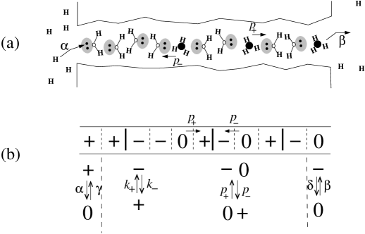
The transition rules are constrained by the orientation of the waters at each site and are defined in Fig. 1b. A proton will enter the first site () from the left reservoir and protonate the first water molecule with rate only if the hydrogens of the first water is pointing to the right (such that its lone-pair electrons are left-pointing, ready to accept proton from the left reservoir). Similarly, if a proton exits from the first site into the left reservoir (with rate ), it leaves the remaining hydrogens right-pointing. The analogous rules hold for the last site with exit and entrance rates and respectively. The entrance rates and are functions to the proton concentration in the respective reservoirs as well as local electric potential gradients near the pore mouths. In the pore interiors, a proton at site can hop to the right(left) with rate only if the adjacent particle is a right(left)-pointing, unprotonated water molecule. If such a transition is made, the remaining water molecule at site will be left(right) pointing. Physically, as a proton moves to the right, it leaves a decaying trail of particles to its left. A left moving proton leaves a trail of particles to its right. These trails of or particles are unable to accept another proton from the same direction. Clearly, protons can successively follow each other only if the waters can reorient without being protonated. The water reorientation rates are denoted (cf. Fig. 1b). The rate-limiting steps in steady-state proton transfer across biological water channels is thought to be associated with water flipping.
This water wire conduction model resembles the two species ASEPs treated by Evans et al. [21] if one identifies protons with vacancies, and allows the and clkass particles to interconvert with rates . Moreover, particles here can only move left, and once they do, get converted to type particles. Similarly, a particle that moves to the right becomes a particle. The allowed moves are . Although the master equation can be formally defined in terms of the probability for a given configuration , I have failed to discover an analytical result for the steady state current proton () current using matrix product methods [8, 15, 17, 18]. Since it is not always possible to find a finite dimensional matrix product representation, particularly for open boundaries, many practical applications, such as multipecies pore transport [7], must be treated using mean field approximations or numerical simulations. For the single species ASEP, the mean field result for the steady-state current is exact in the limit, although the site occupancies do not agree with those from the exact solution. Therefore, a mean field theory in the present problem may shed light on the steady-states. We will obtain mean field analytic expressions that can be compared with numerical simulations.
3 Mean field approximation
For one-dimensional nearest lattice site hopping models, the mean-field assumption states that the probability that the system is in a configuration with occupancy and factors into a product of single particle probabilities:
| (1) |
where . The master equations thus become
| (2) | |||
| (3) | |||
| (4) |
where are the individual probabilities that site is occupied by a particle in state . Conservation at each site requires . In the present treatment, we will assume that are independent of neighboring configurations , i.e. that the transition rates are local and do not depend interaction with the states of neighboring sites. Within the mean field approximation, the instantaneous current of protons between sites and is
| (5) |
while the currents at the left and right boundaries are
| (6) |
Upon defining steady-state particle occupancies over their probabilities, , , and . The steady-state currents are thus
| (7) |
and
| (8) |
In steady-state, all currents have to be identical, . Thus, the constant, internal steady-state current (7) reads
| (9) |
while the equation for reads
| (10) |
From (10), we see that is constant along the chain. Upon imposing particle conservation, ,
| (11) |
| (12) |
| (13) |
| (14) |
where
| (15) |
We can now write (14) as a recursion relation of the form
| (16) |
Upon redefining
| (17) |
we find the recursion relation for :
| (18) |
Except for the more complicated dependence of on , the recursion relation (18) is identical to that used in analyzing the mean-field properties of the totally and partially asymmetric exclusion process for a single species [14, 18]. The solution to the difference equation (18) is [14]
| (19) |
where
| (20) |
Similarly, the boundary occupations can be readily found by substituting (12) and (13) into (17) and solving for .
3.1 Symmetric limit
First consider the totally symmetric case where and the “unbiased” current vanishes as . One important realisation of this condition is and , corresponding to waters without left-right preference along the wire, and to the absence of pondermotive forces on the wire protons. We name this limit the symmetric limit because the net bias on internal protons vanish 111In the proton conduction literature, the term “symmetric” is often used to denote symmetric solutions, or equal proton concentrations in the two reservoirs. The current in this case is driven by an externally imposed transmembrane potential. The proton current is driven entirely by a proton number density difference between the two reservoirs, i.e. an asymmetry in injection and extraction rates at the boundaries. Upon iterating Eqn (16) with ,
| (21) |
From the boundary conditions at , we obtain an implicit equation for :
| (22) |
where the are functions of given by Eqns. (15). A closed analytic expression can be found as an asymptotic expansion about large using the ansatz
| (23) |
where the are -independent coefficients that are functions of the kinetic rates. To lowest order,
| (24) |
At , (22) determines and the steady-state current
| (25) |
When , the current (25) in the limit of small proton concentration differences can be expanded in powers of ,
| (26) |
reflecting a current driven by the effective difference in boundary injection rates. Finally, in the large and limit,
| (27) |
3.2 Asymmetric limits
For driven systems, where , a finite current persists in the limit. Mean field currents are found from the fixed points of the recursion relation (18). The average particle occupations at each site can be then be reconstructed from the solution to . In analogy to the single-species partially asymmetric process, the condition leads to a single fixed point that determines , via a quadratic equation which is solved by
| (28) |
For the sake of simplicity, we assume and furthermore are such that . Clearly (since must be less than the smallest rate in the entire process) and . In the limit , only provides a physical solution,
| (29) |
For a purely asymmetric process and the maximal current in this model approaches the analogous maximal current expression of the single species ASEP,
| (30) |
except for modification by the factor representing the fraction of time the site to the immediate right of a proton is in the state.
Another possibility is which leads to two fixed points, one stable at and one unstable at . Following [14] and [18], we set in one case the left occupation to the stable value which self-consistently determines the current via , while equation (12) determines . Thus is solved by
| (31) |
where
| (32) |
The injection rate-limited current (31) depends only upon . Upon iterating, we find the regime of validity for is determined by . Thus, the currents can arise only when and and correspond to a low proton density () phase.
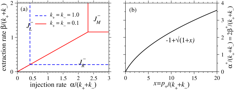
Another limit of steady-state currents corresponds to the high density phase where , which is found from with
| (33) |
Equation (33) is also easily deduced from the solutions and the symmetry properties of , and under the transformation . The solutions hold only if and correspond to a high proton density phase. Although the currents represented by equations (28), (31), (33), and their associated regimes of validity define a potentially rich mean field current phase diagram, significant simplification, where simpler expressions can be obtained, is achieved by restricting ourselves to the totally asymmetric regime where . In this case, , and . Upon using and given by (12) and (13), the currents (28), (31), and (33), and their regimes of validity become
| (34) |
where
| (35) |
4 Monte-Carlo simulations
We now compare mean field results from both the symmetric and asymmetric limits with their corresponding steady-state currents obtained from lattice Monte Carlo (MC) simulations. The simulation was implemented by defining sites corresponding to the interior pore sites, plus the two reservoirs. At each time step, one of the sites was randomly chosen and a transition attempted. Transitions were accepted according to the Metropolis algorithm. At the next time step, another site was randomly chosen. The occupation at each reservoir end site was set to so that protons were always ready to be injected with probability corresponding to the rates . To obtain low noise steady-state values for the occupations and currents, instantaneous currents across all boundaries were averaged over time steps.
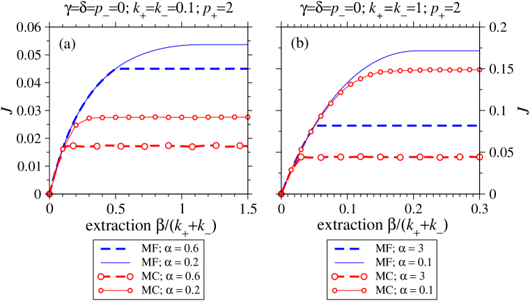
Figures 3a,b show slices (for , , and fixed ) through the phase diagram of the totally asymmetric case (Fig. 2). The mean field currents are represented by the thin solid and thick dashed curves for different values of in each plot. Mean field theory seems to predict a first order transdition between the and phases and a higher order transition to the phase. The curves labelled with symbols represent steady-state currents computed from the MC simulations for the same fixed values of . The mean field solutions always overestimate the currents with the error especially bad for small (compare Fig. 3a with Fig. 3b). This suggests correlations are suppressed when water flipping is fast, rendering the mean field approximation more accurate. A similar qualitative trend arises in the symmetric case.
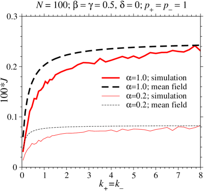
Figure 4 shows the steady-state currents for in the special symmetric case () as a function of the equal flip rates . The asymptotic mean-field currents for () and () are plotted with thin and thick dashed curves, respectively. The mean-field results again overestimate the steady-state current , and become increasingly accurate for large flip rates. The limit in which mean field theory is asymptotically exact gives
| (36) |
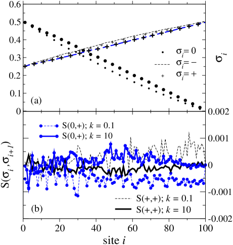
Site occupations depicted in Fig. 5a clearly indicate the absence of boundary layers in the symmetric limit. The proton concentration is nearly linear along the chain and is fairly insensitive to the flipping rate . Only for small (thin lines, small symbols) does the profile deviate slightly from being linear. Not surprisingly, the mean field result for the steady-state current is substantially more accurate when is large. Figure 5b shows the correlations
| (37) |
as functions of the lattice site . We plot and (circles) for both (thin dashed lines) and (thick solid lines). Correlations containing do not vary appreciably when is changed. Note that for is larger than for . The larger flipping rates wash out the correlations and suppresses . Conversely, for small is negative since is a relatively fast step that destroys the configuration. When is large, this negative correlation is also supressed.
Figures 6 contrasts concentration difference driven currents and potential difference driven currents. In figure 6a, is plotted as a function of for and . The current is always sublinear with respect to and increases for small, increasing . For larger , the current saturates as the rate limiting step becomes the forward hopping rate .
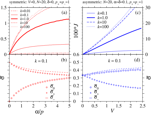
The site occupancies, averaged over the entire chain, are plotted in Fig. 6b. The curves plot , , and , representing the chain-averaged proton, type, and type particle densities, respectively. As the proton entrance rate is increased, the proton concentration in the pore increases at the expense of both and particles. However, since the current to the right increases, the average population of particles decreases faster than that of the particles. For larger , the difference between and occupations vanishes as the high flip rate equalizes their probabilities; the only small remaining difference arises from the occasional passing of a proton converting to .
For potential driven flow, the forward and backward hopping rates were modified according to
| (38) |
As a function of , the current can appear to be sublinear or superlinear depending on the voltage regime (Fig. 6c). For small and sufficiently large , the rate limiting steps are the flips and the current is sublinear. The voltage-driven average particle densities for (Fig. 6d) also show increasing proton concentrations and decreasing particle densities.
5 Conclusions
We have formulated an interacting, three-species transport model (epitomized in Fig. 1) which is motivated by the Grotthuss mechanism [24] of proton transfer along water wires. The dynamics resemble those of two-species ASEPs but with important differences that give rise to very different behavior. Our main results are summarized by analytic expressions for the steady-state currents derived within a mean-field approximation. Currents in both symmetric (equations 25 and 26) and asymmetric regimes (equations 28, 31, and 33) were found, with phases in the totally asymmetric limit (equation 34) analogous to those of the standard ASEP. Monte-Carlo simulation agree with mean field analyses only in the limit of large flipping rates . Although qualitatively correct, the totally asymmetric mean field currents described by the phase diagram in Fig. 2, always overestimates the actual currents, as shown in Fig. 3. As apparent from Figs. 3,4, steady-state currents in both symmetric and asymmetric limits are very sensitive to subtle variations in average occupation and minute differences in nearest neighbor correlations plotted in Fig. 5.
Our model does not include many important interactions that may be important in real physical systems. Examples include dipole-dipole interactions between adjacent waters, hydronium-hydronium repulsion between two adjacent protons, and potential induced ordering fields that preferentially orient the water dipoles. These effects can be readily incorporated by considering next-nearest neighbor interactions. The more complicated interaction energy can be used in weighting Monte-Carlo acceptance steps.
A salient experimental finding in membrane potential-driven water wire proton conduction is the crossover from sublinear curves to superlinear curves as the pH in the two equal reservoirs is decreased [22]. Multiple protons on the water wire have been implicated in the crossover to superlinear behavior. Unlike previous theories [25], our model allows for multiple proton entry into the water wire. In addition to finding a wider regime of superlinearity for large , we also found (not shown) stronger superlinearity when the injection rates () were large relative to extraction rates (). These results of the simple lattice model display a number of different regimes, provide relative estimates for fundamental tranition rates, and will serve as a starting point for more complicated models of measured characteristics [26].
Acknowledgments The author thanks G. Lakatos and J. Rudnick for helpful comments and suggestions.
References
References
- [1] Krug J and Spohn H 1991 Kinetic Roughening of growing surfaces Solids Far From EQuilibrium ed C Godreche (Cambridge University Press: Cambridge)
- [2] Kandel D and Mukamel D 1992 Defects, interface profile and phase transitions in growth models Europhys. Lett. 20, 325
- [3] Schreckenberg M, Schadschneider A, Nagel, K and Ito N 1995 Phys. Rev. E51 2339
- [4] Karimipour, V 1999 Multispecies asymmetric simple exclusion process and its relation to traffic flow Phys. Rev. E59 205
- [5] Kukla V, Kornatowski J, Demuth D, Girnus I, Pfeifer H, Rees L, Schunk S, Unger K, and Kärger J 1996 Science 272 702
- [6] Chou T 1999 Kinetics and thermodynamics across single-file pores: solute permeability and rectified osmosis, J. Chem. Phys., 110, 606-615
- [7] Chou T and Lohse D 1999 Entropy-driven pumping in zeolites and ion channels Phys. Rev. Lett. 82(17), 3552-3555
- [8] Sandow S 1994 Partially asymmetric exclusion process with open boundaries Phys. Rev. E50 2660-2667
- [9] MacDonald J T, Gibbs J H, and Pipkin A C 1968 Biopolymers 6 1
- [10] MacDonald J T and Gibbs J H 1969 Biopolymers 7 707
- [11] Jülicher F, Ajdari A and Prost J 1997 Rev. Mod. Phys. 69 1269
- [12] Vilfan A, Frey E and Schwabl F 2001 Relaxation kinetics of biological dimer adsorption models Europhys. Lett. 56 420-426
- [13] Kolomeisky A B 2001 Exact Results for Parallel Chains Kinetic Models of Biological Transport J. Chem. Phys. 115 7253-7259
- [14] Derrida B, Domany E and Mukamel D 1993 Exact solution of a 1D asymmetric exclusion model using a matrix formulation J. Phys. A 26, 1493-1517
- [15] Derrida B, Evans M R, Hakim V and Pasquier V 1992 An Exact Solution of a One-Dimensional Asymmetric Exclusion Model with Open Boundaries J. Stat. Phys. 69 667-687
- [16] Derrida B and Evans M R 1997 The asymmetric exclusion model: Exact results through a matrix approach Nonequilibrium Statistical Mechanics in One Dimension, (Cambridge University Press, Cambridge).
- [17] Derrida B 1998 An exactly soluble non-equilibrium system: The asymmetric simple exclusion process Physics Reports 301 65-83
- [18] Essler F H and Rittenberg V 1996 Representations of the quadratic algebra and partially asymmetric diffusion with open boundaries J. Phys. A: Math. Gen. 29 3375-3407
- [19] Mallick K, Mallick S, and Rajewsky, N 1999 Exact solution of an exclusion process with three classes of particles and vacancies J. Phys. A: Math. Gen. 32 8399
- [20] Karimipour V 1999 A multi-species asymmetric exclusion process, steady state and correlation functions on a periodic lattice Europhysics Letters bf 47 304-310
- [21] Evans M R, Foster D P, Godreche C, and Mukamel D 1995 Spontaneous symmetry breaking in a one-dimensional driven diffusive system Phys. Rev. Lett. 74 208-211
- [22] Eisenman G, Enos B, Sandblom J and Hägglund J 1980 Gramicidin as an example of a single-filing ionic channel Ann. N.Y. Acad. Sci. 339 8-20
- [23] Deamer D W 1987 Proton permeation of lipid bilayers J. Bioenerg. Biomembr. 19 457-479
- [24] Grotthuss C J T 1806 Sur la décomposition de l’eau et des corps qu’elle tient en dissolution l’aide de l’électricité galvanique Ann. Chim. LVIII 54-74
- [25] Schumaker M F, Poms R and Roux B 2001 Framework Model For Single Proton Conduction through Gramicidin, Biophys. J. 80 12-30
- [26] Phillips L R, Cole C D, Hendershot R J, Cotten M, Cross T A and Busath D D 1999 Noncontact Dipole Effects on Channel Permeation. III. Anomalous Proton Conductance Effects in Gramicidin Biophys. J. 77 2492-2501