On the Red-Green-Blue Model

Abstract

We experimentally study the red-green-blue model, which is a sytem of loops obtained by superimposing three dimer coverings on offset hexagonal lattices. We find that when the boundary conditions are “flat”, the red-green-blue loops are closely related to SLE₄ and double-dimer loops, which are the loops formed by superimposing two dimer coverings of the cartesian lattice. But we also find that the red-green-blue loops are more tightly nested than the double-dimer loops. We also investigate the 2D minimum spanning tree, and find that it is not conformally invariant.

I Introduction

We investigate the red-green-blue (RGB) model, which was introduced by Benjamini and Schramm. An RGB configuration is a system of the loops on a region of the triangular lattice, which is obtained by superimposing three perfect matchings (or dimer coverings) on offset hexagonal lattices as shown in Figure 1. The sites of the triangular lattice may be three-colored so that no two adjacent sites have the same color. If we delete the sites of a given color (say blue), then the sites of the other two colors (red and green) form a hexagonal lattice on which we can construct a random perfect matching (the blue perfect matching). When we superimpose the red, green, and blue perfect matchings, each vertex is matched with one neighboring vertex of each of the other two colors. Since each vertex has degree two, an RGB configuration consists of closed loops, and each loop has an orientation if we follow the edges in the order red to green to blue.

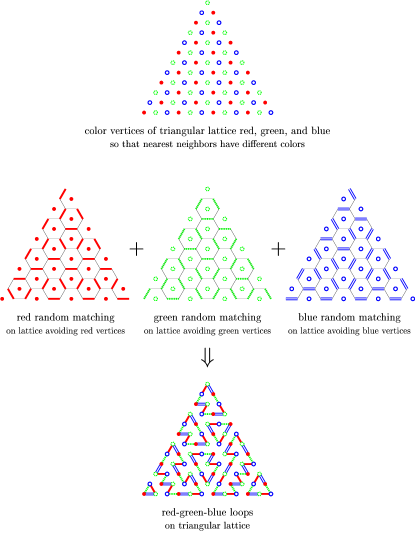
Figure 1: The red-green-blue (RGB) model on a triangular region of side length $12$ ($L=4$). The three color classes of vertices are balanced along the boundary, so the boundary conditions are “flat”.

It is worth remarking that the boundary conditions of dimer systems can have a profound impact on the behavior of dimers even far within the interior of a region Cohn et al. (1996, 1998, 2001). There are height functions associated with dimer configurations on the cartesian lattice Levitov (1990); Zheng and Sachdev (1989) and hexagonal lattice Blöte and Hilhorst (1982) (see also Thurston (1990); Propp (2002)). If there is an imbalance between the different colors of vertices along the boundary, then the height along the boundary will be “tilted”, and this affects the dimers throughout the region. Consequently, the behavior of the RGB model on regions with tilted boundary conditions could be different from the behavior of the RGB model on the regions that we consider here, where the three color classes along the boundary are balanced (“flat” boundary conditions).

In earlier work, Kenyon and the author Kenyon and Wilson (1999) found experimentally that the fractal dimension of these loops is $3/2$. Here we report on additional experiments, where we find that the winding angle variance at a typical point on a loop is $1\times\log D$ where $D$ is the diameter of the loop, and that the system of loops appears to be conformally invariant. These properties suggest that the RGB loops are closely related to stochastic Loewner evolution Schramm (2000) with parameter $\kappa=4$ (SLE₄), and that the RGB loops belong to the same universality class as the contours of 2D Fortuin-Kasteleyn Fortuin and Kasteleyn (1972) clusters at criticality when $q=4$, and the loops formed in the double-dimer (or “double-domino”) model Kondev and Henley (1995), which in turn are thought to correspond to the “contours” of a Gaussian free field Kondev and Henley (1995). However, the system of RGB loops does not have the same limiting behavior as the system of double-dimer loops, because we also find that the RGB loops are more tightly nested than the double-dimer loops.

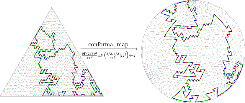
Figure 2: The RGB model on the triangular domain ($L=20$) is conformally mapped to a disk. The inverse conformal map, from the disk to the triangle, is the hypergeometric function shown in the diagram. If the RGB model is conformally invariant, then the loops in disk will be rotationally invariant.

II Generating RGB configurations

To generate an RGB configuration of a region, we need to generate dimer coverings of three regions of the hexagonal lattice. There are many ways to generate dimer coverings of the the hexagonal lattice, but the fastest of these is based on a generalization of Temperley’s bijection Temperley (1974) between spanning trees and dimers. To generate the perfect matchings on the hexagonal lattice, the corresponding spanning trees are on a directed triangular lattice (see Kenyon et al. (2000) for details), and these spanning trees may be quickly generated using an algorithm based on loop-erased random walk Propp and Wilson (1998). This generalized-Temperley bijection only works for regions of the hexagonal lattice that have certain special (very flat) boundary conditions, so we can only expect to use it to generate RGB configurations of certain nice regions. One region where we can use spanning trees to rapidly generate RGB configurations is the equilateral triangle with side length $3L$ (Figures 1 & 2).

III Windiness of RGB loops

We recall the definition of the windiness of a loop used in Wieland and Wilson (2002). Consider an ant which travels along the loop; after the ant has just traversed a given edge in the loop, before traversing the next edge it will either turn left $120^{\circ}$, turn right $120^{\circ}$, or not turn at all. If we keep track of the total turning (measured in radians) when the ant travels from point $A$ to point $B$ on the loop, then this is (approximately) the winding angle between points $A$ and $B$. When the ant travels all the way around the loop, it has turned $\pm 360^{\circ}$, so to make the winding angle between points $A$ and $B$ independent of the number of times that the ant travels around the loop and the direction of travel, we adjust the total turning (measured in radians) by $2\pi\times[\text{\# steps between $A$ and $B$}]\div[\text{length of loop}]$. To define the winding angle at a given point $X$ relative to the global average direction, we pick an arbitrary point $A$, compute the winding angle from $A$ to $X$, and subtract a global constant so that the average winding angle at points on the curve is $0$.

When we measure the variance in the winding angle at random points along the longest loop in the RGB configuration in a region of order $L$, we find that the variance grows like $1\times\log L$ — so in the notation of Wieland and Wilson (2002), $\kappa_{2}=1$. This winding angle variance coefficient of 1 also shows up in in the contours of FK clusters at criticality when $q=4$, and other related models such as the double-dimer model, and SLE₄ (see Duplantier and Saleur (1988); Wieland and Wilson (2002); Duplantier and Binder (2002)).

IV Conformal invariance of RGB loops

Since there is only one region, the equilateral triangle, for which we can rapidly generate RGB configurations, this makes the testing of conformal invariance somewhat interesting. The test that we use is similar in spirit to the tests used by Schramm to test the conformal invariance of the uniform spanning tree. We conformally mapped the RGB model on the triangular domain to a circular domain, as shown in Figure 2. If the RGB model with flat boundary conditions were conformally invariant, then it must be that after we map a region to the disk, the resulting system of loops would be rotationally invariant. But if conformal invariance failed to hold, then there would be no particular reason to believe that the loops mapped to the disk would be rotationally invariant. After all, referring to Figure 2, the points in the disk to which the corners of the triangle are mapped certainly look different than other points in the disk, so a priori we would expect the image in the disk to be anisotropic if the RGB model were not conformally invariant. As we shall see, the minimum spanning tree model fails this test, so this test is a nontrivial test of conformal invariance.

To test the rotational invariance of the image of the RGB model in the disk, we singled out the outermost loop surrounding the center of the circular domain, and collected statistics on its furthest extents in the $\pm x$- and $\pm y$-directions. If the loops in the RGB model are conformally invariant, then these four random variables would be equidistributed. But otherwise, there would be no particular reason to believe that any of these random variables (other than the first two) would have the same distributions. As shown in Figure 3, the cumulative distribution functions for these four random variables appear to coincide, so we conclude that the RGB model appears to be conformally invariant.

Figure 3: In the RGB model ($L=1024$), the outermost loop surrounding the center point is selected, and conformally mapped to the disk. The image of this loop appears to be rotationally invariant, in particular, the empirical cumulative distribution functions for furthest extents of the loop in the $x$-direction, $y$-direction, $-x$-direction, and $-y$-direction appear to coincide.

V Conformal non-invariance of minimum spanning trees

To evaluate the efficacy of our conformal invariance test, we applied it to two additional models: the minimum spanning tree and uniform spanning tree models. The minimum spanning tree (MST) is formed by assigning uniformly random edge weights to the edges of the cartesian lattice, and picking the spanning tree (connected acyclic subset of

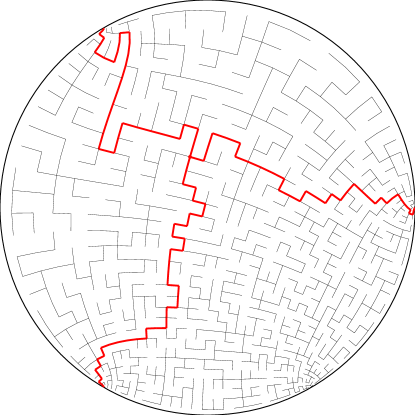
Figure 4: The minimum spanning tree (MST) on the $32\times 32$ square grid, mapped conformally to the disk so that three of the corners of the square are mapped to the cube roots of unity. The paths connecting these corners is highlighted; the triple point $T$ is the point contained in all three paths.

edges) which minimizes the total weight. The uniform spanning tree (UST) is simply a spanning tree chosen uniformly at random from all spanning trees.

Figure 4 shows the MST of a square grid after it is conformally mapped to the unit disk, with three of the corners mapped to the three cube roots of unity. To test the rotational invariance of the MST after it is mapped to the disk, we looked at the paths connecting the three points at the cube roots of unity (highlighted in Figure 4), and focused on the “triple-point” $T$ contained in all three paths. If the image of MST in the disk were isotropic, then $T$, $e^{2\pi i/3}T$, and $e^{4\pi i/3}T$ would be equidistributed. However, as Figure 5 illustrates, these variables are not equidistributed, so we conclude that the MST is not conformally invariant. The conformal non-invariance of the MST is surprising, given the close relationship between the MST and invasion percolation Chayes et al. (1985), the close relationship between invasion percolation and percolation, and the conformal invariance of percolation Langlands et al. (1994); Cardy (1992); Smirnov (2001).

Figure 5: The distribution of the triple point $T$ for the MST (on the $1024\times 1024$ grid) is not symmetric under $120^{\circ}$ rotations, as it would be if the MST were conformally invariant. ($\omega=\exp(2\pi i/3)$.)

In contrast to the MST, the UST passes this test, as shown in Figure 6. The triple point $T$ connecting three boundary points of the UST is already known to be conformally invariant Kenyon (2000), and indeed the entire UST process is now known to be conformally invariant Lawler et al. (2001).

Figure 6: In contrast, the distribution of the triple point $T$ for the UST (on the $1024\times 1024$ grid) passes this conformal invariance test. Kenyon Kenyon (2000) has proven that the triple point for UST is in fact conformally invariant (see also Lawler et al. (2001)).

Thus we learn not only that the minimum spanning tree is not conformally invariant, but that this test is a nontrivial test of conformal invariance.

VI Nesting of RGB loops

For a scale-invariant loop model on a region of side length $L$, we would expect the number of loops surrounding a point to scale as $\text{const.}\times\log L$. The value of this constant is a measure of how deeply nested the loops are. For the double-dimer model, Kenyon Kenyon (1997) proved that this nesting constant is $1/\pi^{2}$. We measured the nesting constant of the RGB loops, and found that it is $20\%$–$25\%$ larger than the double-dimer nesting constant, but we do not have a guess for its exact value. Figure 7 shows that the outermost red-green-blue loops are in a sense larger than the outermost double-dimer loops, which is consistent with the red-green-blue loops being more tightly nested within one another.

Figure 7: Comparison of the outermost loop surrounding in the origin within the red-green-blue and double-dimer models. The cdf for the size of the RGB loop is smaller than the corresponding CDF for the DD loop, so in this sense the outermost RGB loop is larger than the outermost double-dimer loop. There is a good chance that the outermost RGB loop approaches the boundary quite closely, as in Figure 2.

VII Conclusions

Our experiments indicate that the loops of the RGB model (with flat boundary conditions) are conformally invariant and have windiness constant $1$. Earlier experiments Kenyon and Wilson (1999) have indicated that the fractal dimension is $3/2$. These properties suggest that RGB loops belong to the same universality class as double-dimer loops, the fully-packed-loop model with $n=2$, and the contours of critical FK clusters with $q=4$, and are closely related to SLE₄. However, the system of RGB loops (not just individual loops) differs from the system of double-dimer loops, because the loops are nested within one another more tightly.

References

- Cohn et al. (1996) H. Cohn, N. Elkies, and J. Propp, Duke Math. Journal 85, 117 (1996).
- Cohn et al. (1998) H. Cohn, M. Larsen, and J. Propp, New York J. Math. 4, 137 (1998).
- Cohn et al. (2001) H. Cohn, R. W. Kenyon, and J. G. Propp, J. AMS 14, 297 (2001).
- Levitov (1990) L. S. Levitov, Phys. Rev. Lett. 64, 92 (1990).
- Zheng and Sachdev (1989) W. Zheng and S. Sachdev, Phys. Rev. B 40, 2704 (1989).
- Blöte and Hilhorst (1982) H. W. J. Blöte and H. J. Hilhorst, J. Phys. A 15, L631 (1982).
- Thurston (1990) W. Thurston, American Math. Monthly 97, 757 (1990).
- Propp (2002) J. Propp (2002), eprint math.CO/0209005.
- Kenyon and Wilson (1999) R. W. Kenyon and D. B. Wilson (1999), unpublished.
- Schramm (2000) O. Schramm, Israel J. Math. 118, 221 (2000).
- Fortuin and Kasteleyn (1972) C. Fortuin and P. Kasteleyn, Physica 57, 536 (1972).
- Kondev and Henley (1995) J. Kondev and C. L. Henley, Phys. Rev. Lett. 74, 4580 (1995).
- Temperley (1974) H. N. V. Temperley, in London Math. Soc. Lecture Notes Series #13 (1974), pp. 202–204.
- Kenyon et al. (2000) R. W. Kenyon, J. G. Propp, and D. B. Wilson, Electronic J. Combinatorics 7, 591 (2000), paper #R25.
- Propp and Wilson (1998) J. G. Propp and D. B. Wilson, J. Alg. 27, 170 (1998).
- Wieland and Wilson (2002) B. Wieland and D. B. Wilson (2002), manuscript.
- Duplantier and Saleur (1988) B. Duplantier and H. Saleur, Phys. Rev. Lett. 60, 2343 (1988).
- Duplantier and Binder (2002) B. Duplantier and I. Binder (2002), eprint cond-mat/0208045.
- Chayes et al. (1985) J. Chayes, L. Chayes, and C. M. Newman, Commun. Math. Phys. 101, 383 (1985).
- Smirnov (2001) S. Smirnov (2001), URL http://www.math.kth.se/~stas/papers/percol.ps.
- Langlands et al. (1994) R. Langlands, P. Pouliot, and Y. Saint-Aubin, Bull. AMS 30, 1 (1994).
- Cardy (1992) J. Cardy, J. Phys. A 25, L201 (1992).
- Kenyon (2000) R. Kenyon, J. Math. Phys. 41, 1338 (2000).
- Lawler et al. (2001) G. F. Lawler, O. Schramm, and W. Werner (2001), eprint math.PR/0112234.
- Kenyon (1997) R. Kenyon, Annales de l’Institut Henri Poincaré – Probabilités et Statistiques 33, 591 (1997).