Effective mass analysis of Bose-Einstein condensates in optical lattices —
stabilization and levitation

Abstract

We investigate the time evolution of a Bose-Einstein condensate in a periodic optical potential. Using an effective mass formalism, we study the equation of motion for the envelope function modulating the Bloch states of the lattice potential. In particular, we show how the negative effective mass affects the dynamics of the condensate.

I Introduction

The dynamics of classical and quantum systems in periodic potentials is a central paradigm of physics, finding applications from condensed matter physics to optics, and from nonlinear dynamics to atomic and to plasma physics. In recent years, the experimental and theoretical study of quantum-degenerate atomic systems in periodic potentials has opened up new avenues of investigation. In particular, Bose-Einstein condensates are a macroscopic quantum system that is amenable to exquisite experimental control. As a result, many phenomena studied in solid state systems can be re-examined in a more direct and dramatic fashion. Even more importantly perhaps, it is now possible to realize experimentally model systems that had previously been the object of considerable theoretical studies, but were all but impossible to test experimentally. One particularly beautiful example is the experimental realization of the Hubbard model leading to the demonstration of the superfluid to Mott insulator transition in a Bose condensate of ⁸⁷Rb atoms mott .

The first experiments involving the dynamics of Bose-Einstein condensates (BEC) in periodic potentials were carried out by Anderson and Kasevich, who used this approach to demonstrate a mode-locked atom laser modelock and observe atomic Josephson oscillations modelock ; josephson . The list of phenomena that were subsequently experimentally demonstrated and/or theoretically investigated includes the generation of atomic number squeezing squeez , the observation of the superfluid-Mott insulator phase transition, the generation of discrete dis or gap solitons gap , the prediction of modulational instabilities stability and superfluid flow flow , the observation of Bloch oscillations blochosc , the analysis and observation of coherent acceleration acceleration , studies of magnetism mag , etc.

It is well known that a particle confined to an infinite periodic potential and acted upon by an external force behaves as if possessing an effective mass that can be substantially different from its true mass, and may even take negative values. In particular, it is this property that is at the core of proposals to generate bright matter-wave solitons in BECs with repulsive interactions gap . The purpose of the present paper is to extend these studies by analyzing the temporal evolution of a condensate in the periodic potential provided by an optical lattice. The initial state of the condensate is chosen to be a (approximate) Bloch state modulated by a slow-varying Gaussian envelope, and we compare two situations where the Bloch state is either associated with a positive or a negative effective mass. We show that in situations where the dynamics of the condensate is well approximated by a negative effective mass, the periodic potential can lead to the stabilization of an otherwise unstable condensate. We also demonstrate theoretically the levitation of condensates of negative effective masses. These studies further allow us to determine the impact of self-interactions and of finite condensate widths on the general usefulness of the effective mass concept.

The paper is organized as follows. Section II gives a brief review of the linear problem of a particle inside a periodic sinusoidal potential and introduces the concept of effective mass. Section III applies and extends these ideas to the dynamics of a BEC in an optical lattice. We discuss the equation of motion for the slowly varying condensate envelope function, from which we can gain useful physical insights into the dynamics of the system. A full numerical solution is presented in Sec. IV, which demonstrates in particular the stabilization and the levitation of a condensate of negative effective mass, in agreement with the prediction of Sec. III. Finally, Section V presents concluding remarks on the usefulness of the effective mass concept and an outlook.

II Linear properties of infinite periodic potential

In this section, we briefly review important aspects of the linear problem of a particle of mass $m$ inside a one-dimensional infinite periodic potential of the form

$$V(x)=V_{0}\cos^{2}(k_{0}x),$$ (1)

with corresponding time-independent Schrödinger equation

$$\left[-\frac{\hbar^{2}}{2m}\frac{d^{2}}{dx^{2}}+V_{0}\cos^{2}(k_{0}x)\right]\phi(x)=E\phi(x).$$ (2)

We proceed by introducing the dimensionless quantities

$$\theta=k_{0}x;\;\;\;b=\frac{2mE}{\hbar^{2}k_{0}^{2}};\;\;\;h^{2}=\frac{2mV_{0}}{\hbar^{2}k_{0}^{2}},$$ (3)

in terms of which Eq. (2) becomes

$$\frac{d^{2}\phi}{d\theta^{2}}+\left(b-h^{2}\cos^{2}\theta\right)\phi=0.$$ (4)

Eq. (4) has the form of Mathieu’s equation, whose solutions are well known mathieu . As a warm-up we sketch out the main features of its solutions which, according to Bloch’s theorem, must be of the form

$$\phi_{n,s}(\theta)=e^{is\theta}F_{n}(\theta),$$

where $s$ is real and arbitrary (in standard textbook language, $s=k/k_{0}$ where $\hbar k$ is the quasi-momentum). In our scaled units, the periodic functions $F_{n}(\theta)$ have a period of $\pi$. The energy spectrum associated with the periodic potential $V(\theta)$ exhibits a band structure familiar from solid state physics. Each value of $s$ gives a discrete spectrum whose structure is periodic with respect to $s$. This property allows one to restrict the discussion to the first Brillouin zone, $-1<s\leq 1$. As $s$ is increased within that zone, the energy levels trace out curves that are restricted to a small energy band. We restrict our discussion to the first two bands, as depicted in Fig. 1(a). Note that although the probability distribution $|\phi|^{2}$ is a periodic function of $\theta$, $\phi$ itself is not periodic unless $s$ takes integer values — e.g., at the center or the edges of the Brillouin zone. For a detailed discussion of the solutions to Eq. (4), see e.g. Ref. mathieu .

For $s=0$ or 1, the eigenstates of the Mathieu’s equation are periodic and take the form of standing waves. In particular, at the edge $s=1$ of the first Brillouin zone, the wave functions $\phi_{n,s}$ for the first two energy bands, $n=1,2$, can be expressed as the Fourier series

$$\phi_{1,s=1}(\theta)=\sum_{n=0}^{\infty}A_{2n+1}\sin(2n+1)\theta,$$ (5)

and

$$\phi_{2,s=1}(\theta)=\sum_{n=0}^{\infty}B_{2n+1}\cos(2n+1)\theta,$$ (6)

where

$$G_{2n+1}=k_{2n-1}-\frac{1}{G_{2n-1}},\;\;\;n>1,$$

$$k_{n}=(4b-2h^{2}-4n^{2})/h^{2},$$

$$G_{2n+1}=A_{2n+1}/A_{2n-1},\;\;\;{\rm or}\;\;\;B_{2n+1}/B_{2n-1},$$

and $A_{3}=k_{1}+1$, $B_{3}=k_{1}-1$.

The effective mass, $m^{*}$, which characterizes the response of the particle to external perturbations, is defined as

$$m^{*}=\frac{\hbar^{2}}{\partial^{2}E/\partial k^{2}}=\frac{2m}{\partial^{2}b/\partial s^{2}}.$$ (7)

Fig. 1(b) shows the variation of the effective mass of the first two bands with the quasi-momentum. One observes that it is near infinite (i.e., $1/m^{*}=0$) for certain values of the quasi-momentum $s$, and even becomes negative in certain regions of the zone. In more than one dimension, $m^{*}$ acquires a tensorial character, with elements given by

$$m^{*}_{\mu\nu}=\frac{\hbar^{2}}{\partial^{2}E/(\partial k_{\mu}\partial k_{\nu})}\,.$$

In the next section, we apply the effective mass formalism to the case of a self-interacting Schrödinger field described by the Gross-Pitaevskii equation. Specifically, we show that a BEC prepared in a Bloch state with negative effective mass behaves as if the signs of its self-interaction and of the external confining potential had been reversed.

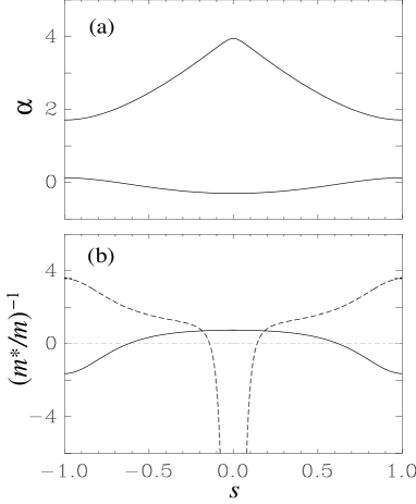
Figure 1: (a) Dimensionless energy $\alpha=b-h^{2}/2$ and (b) scaled reciprocal effective mass $m/m^{*}$ for the first two bands as a function of the normalized quasi-momentum $s$. In (b), the solid and dashed lines refer to the first and second band, respectively. For this calculation, $h^{2}=3.2$.

III Effective mass equation

We consider a BEC in a sinusoidal optical lattice potential. Near zero temperature, the system is described to an excellent degree of approximation by a time-dependent Gross-Pitaevskii equation for the normalized condensate wave function $\psi({\bf r},t)$, generalized to include the effects of three-body collisions,

$$i\hbar\frac{\partial\psi({\bf r},t)}{\partial t}=\left[-\frac{\hbar^{2}}{2m}\nabla^{2}+V({\bf r})+U({\bf r})+Ng|\psi|^{2}-iN^{2}K_{3}|\psi|^{4}\right]\psi({\bf r},t).$$ (8)

Here, $V({\bf r})$ is the periodic lattice potential, $U({\bf r})$ is an additional external potential that is taken to be slowly varying on the scale of the lattice period (e.g., a confining potential), $N$ is the total number of atoms, $g$ is the strength of the nonlinear inter-atomic interaction, and $K_{3}$ gives the rate of three-body recombination loss loss .

We proceed by expanding the condensate wave function $\psi({\bf r},t)$ on the complete set of Bloch functions $\phi_{n{\bf k}}({\bf r})$ that are the stationary solutions of the associated linear Schrödinger equation

$$\left[-\frac{\hbar^{2}}{2m}\nabla^{2}+V({\bf r})\right]\phi_{n{\bf k}}({\bf r})=E_{n{\bf k}}\,\phi_{n{\bf k}}({\bf r}).$$ (9)

The subscripts $n$ and ${\bf k}$ represent the band index and quasi-momentum, respectively. The Bloch functions satisfy the orthonormality condition:

$$\int_{\rm cell}\,d{\bf r}\,\phi_{m{\bf k}}^{*}({\bf r})\,\phi_{n{\bf k}^{\prime}}({\bf r})=\frac{\Omega}{(2\pi)^{3}}\,\delta_{mn}\delta_{{\bf k}{\bf k}^{\prime}}\,,$$

where the integral is taken over a single period of the lattice of volume $\Omega$. Our use of the resulting expansion,

$$\psi({\bf r},t)=\sum_{n,{\bf k}}\,A_{n{\bf k}}({\bf r},t)\phi_{n{\bf k}}({\bf r})e^{-iE_{n{\bf k}}t/\hbar}\,,$$ (10)

is motivated by the the fact that the Bloch functions can capture the rapid oscillations of the condensate wave function, while the slowly varying envelope functions $A_{n{\bf k}}$ will describe the slow center-of-mass motion of the condensate.

The equations of motion for the amplitudes $A_{n{\bf k}}$ are found by inserting the expansion (10) into the generalized Gross-Pitaevskii equation (8). The resulting equations are however of little use if a very large number of $A_{n{\bf k}}$ is required to accurately describe the dynamics of the condensate. Here, we consider a more specialized situation where the matter-wave field is characterized by a central wave vector ${\bf k}_{0}$ corresponding to the mean velocity of the condensate (this would correspond to the carrier wave in conventional optics). Hence, we expand $\psi({\bf r},t)$ in a way reminiscent of the slowly varying envelope approximation of quantum optics as

$$\psi({\bf r},t)=\sum_{n}\,f_{n}({\bf r},t)\phi_{n{\bf k}_{0}}({\bf r})e^{-iE_{n{\bf k}_{0}}t/\hbar}\,.$$ (11)

Inserting Eq. (11) into Eq. (8) and applying the effective mass book or multiple scales sipe methods yields a set of equations governing the time evolution of the condensate envelope functions $f_{n}({\bf r},t)$ steel ,

$$i\hbar\left(\frac{\partial f_{n}}{\partial t}+{\bf v}_{g}\cdot\nabla f_{n}\right)=\left[-\frac{\hbar^{2}}{2m^{*}_{\mu\nu}}\frac{\partial^{2}}{\partial x_{\mu}\partial x_{\nu}}+U({\bf r})+Ng^{\prime}|f_{n}|^{2}-iN^{2}K^{\prime}_{3}|f_{n}|^{4}\right]f_{n}.$$ (12)

The derivation of Eq. (12), the so-called effective mass equation, is given in Appendix A. Here $x_{\mu}$ and $x_{\nu}$ are cartesian components of ${\bf r}$ and we use an implicit summation over repeated indices. The velocity

$${\bf v}_{g}=\frac{1}{m}\langle\phi_{n{\bf k}_{0}}|\hat{\bf p}|\phi_{n{\bf k}_{0}}\rangle,$$ (13)

is the drift velocity of the $n$-th band contribution to the condensate envelope. As shown in Appendix A, it is equal to the gradient of the energy $E_{n{\bf k}}$ with respect to the quasi-momentum ${\bf k}$, evaluated at ${\bf k}_{0}$. We note that ${\bf v}_{g}$ vanishes at the extreme points of the band, in particular at the band edges. The coefficients $g^{\prime}$ and $K^{\prime}$ give the renormalized nonlinear interaction strength and three-body loss rate, respectively. They are given by

$$g^{\prime}=\frac{(2\pi)^{3}}{\Omega}g\,\int_{\rm cell}\,d{\bf r}\,|\phi_{n{\bf k}_{0}}({\bf r})|^{4},$$ (14)

and

$$K^{\prime}_{3}=\frac{(2\pi)^{3}}{\Omega}K_{3}\,\int_{\rm cell}\,d{\bf r}\,|\phi_{n{\bf k}_{0}}({\bf r})|^{6}$$ (15)

The lattice potential $V({\bf r})$ does not appear in these expressions, its effects being already incorporated into the effective mass $m^{*}$ which appears in the first term on the right-hand side of Eq. (12) as well as in the drift term on the left-hand side of that equation.

The effects of a negative mass, $m^{*}<0$, can be immediately inferred from the complex conjugate of Eq. (12),

$$i\hbar\left(\frac{\partial f^{\star}_{n}}{\partial t}+{\bf v}_{g}\cdot\nabla f^{\star}_{n}\right)=\left[-\frac{\hbar^{2}}{2|m^{*}_{\mu\nu}|}\frac{\partial^{2}}{\partial x_{\mu}\partial x_{\nu}}-U({\bf r})-Ng^{\prime}|f^{\star}_{n}|^{2}-iN^{2}K^{\prime}_{3}|f^{\star}_{n}|^{4}\right]f^{\star}_{n}.$$ (16)

This equation shows that as compared to the case of a positive effective mass, the condensate density envelope profile $|f_{n}(t)|^{2}$ evolves now under the influence of an inverted external potential $-U({\bf r})$ and an inverted nonlinearity $-g^{\prime}$. As expected, though, the three-body recombination rate does not change sign and still represents a loss term. The change in sign of $g^{\prime}$ and $U$ leads to a number of consequences. In particular, past work has shown how this property can be exploited to launch bright matter-wave solitons in condensates with positive scattering length gap and induce modulational instability stability . The following section explores further consequences of this property.

IV Effects of Negative effective mass

IV.1 Inverted nonlinearity

We first investigate the effect of an inverted nonlinearity. As is well known, this will change the two-body interaction from being repulsive to attractive, and vice versa. Since condensates with attractive interactions are normally unstable against collapse, the sign change of $m^{*}$ is clearly expected to have a significant effect.

To reduce the scale of the computation, we restrict ourselves to a two-dimensional system consisting of a pancake-shaped condensate whose axial motion is frozen to the trap ground state. (We note that condensates with reduced dimensions have already been realized in the laboratory reduce .) Furthermore, to focus on the effects of the nonlinearity, we assume that except for the lattice potential

$$V(x,y)=V_{0}\,[\cos^{2}(k_{0}x)+\cos^{2}(k_{0}y)],$$ (17)

there is no additional external potential in the transverse dimensions.

The evolution of the transverse component $\psi_{\bot}$ of the condensate wave function is then given by the generalized Gross-Pitaevskii equation

$$i\hbar\frac{\partial\psi_{\bot}}{\partial t}$$

$$= \left[-\frac{\hbar^{2}}{2m}\nabla_{\bot}^{2}+V(x,y)+Ng|\psi_{\bot}|^{2}-iN^{2}K_{3}|\psi_{\bot}|^{4}\right]\psi_{\bot},$$

where

$$\nabla_{\bot}^{2}=\partial^{2}/\partial x^{2}+\partial^{2}/\partial y^{2}.$$

For the initial state of the condensate, we assume a gaussian transverse wave function of the form

$$\psi_{\bot}(x,y,t=0)={\cal N}\,f(x,y)\,\phi_{n{\bf k}}(x,y),$$ (18)

where $f(x,y)=\exp[-(x^{2}+y^{2})/w^{2}]$ is a slowly varying Gaussian envelope function of width $w$, $\phi_{n{\bf k}}$ is a Bloch wave function of the linear Hamiltonian, and the constant ${\cal N}$ normalizes $\psi_{\bot}$ to unity. Figs. 2 and 3 illustrate the dynamics of the condensate for two cases, one corresponding to a negative effective mass and the other to a positive one. We choose the Bloch wave function $\phi_{n{\bf k}}$ associated with a negative effective mass $m^{*}$ as

$$\phi_{n{\bf k}}\sim\sin(k_{0}x)\,\sin(k_{0}y).$$ (19)

This corresponds approximately to the Bloch state at the top of the first energy band, whose full expression is given by $\phi_{1,s=1}$ of Eq. (5). The approximate form (19) retains only the dominant term in the Fourier series (5). Its overlap with $\phi_{1,s=1}$ is larger than 99% for the parameters of our simulations. Similarly, for the state of positive effective mass $m^{*}$ we use

$$\phi_{n{\bf k}}\sim\cos(k_{0}x)\,\cos(k_{0}y),$$ (20)

which corresponds roughly to the Bloch state $\phi_{2,s=1}$ at the bottom of the second band, see Eq. (6). Both states (19) and (20) are located at the edge of the first Brillouin zone, with corresponding drift velocities ${\bf v}_{g}=0$. Hence the center of the condensate stays at $x=y=0$ during the course of its time evolution.

Figure 2: Temporal evolution of the density distribution of a BEC in optical lattice. Lighter shades of grey correspond to higher density. The left (right) panel shows the evolution of a positive (negative) $m^{*}$ state. The dimensionless time is $t$=0, 1, 2, and 3 from the top to bottom. In the plots, the ranges for $x$ and $y$ are from $-30$ to 30. The condensate parameters are $N=50000$, $g=-0.004$, $V_{0}=10$, $k_{0}=3$, $K_{3}=3.9\times 10^{-8}$ and the width of the initial envelope function $w=8$. The units for time, length and energy are $1/\omega$, $\sqrt{\hbar/(m\omega)}$, and $\hbar\omega$, respectively, where $\omega$ is the trap frequency in the axial direction.

The two columns in Fig. 2 show snapshots of the density distribution of the condensate for positive (left column) and negative (right column) effective masses $m^{*}$. In both cases the nonlinear interaction strength $g$ is negative, hence in the absence of the lattice the condensate would be unstable and subject to collapse. This however can be changed if the effective mass of the BEC becomes negative, as demonstrated in the right column. In that case, the condensate behaves as if experiencing a repulsive two-body interaction, its width increasing in time. This is in sharp contrast to the situation for a positive effective mass, in which case the condensate width quickly implodes note . This implosion is characterized by a complex dynamical behavior, such as the formation of atomic “bursts,” observed at later times. (We remark that while an attractive condensate can expand if it possesses a sufficiently large kinetic energy, this is not the case of Fig. 2, where the two initial states have nearly identical kinetic energies.) The collapse dynamics depicted here is rather similar to that of an attractive condensate in a harmonic potential, a system which has gained much interest recently as a result of the capability of tuning the scattering length from positive to negative via Feshbach resonance jila ; saito ; santos . We note however that the use of the generalized Gross-Pitaevskii equation becomes questionable in the regime of extreme collapse. This point though it is important, is not central to our results.

Figure 3: Temporal evolution of the number of atoms in the condensate. The solid (dashed) line is for the positive (negative) $m^{*}$ state. Same parameters as in Fig. 2.

We conclude this section by observing that the number of condensate atoms decreases in time, due to the presence of three-body loss. This is particularly evident for the state with positive effective mass, as shown in Fig. 3. This is as expected, since the atomic density is higher in that case. Finally, we note that as a result of the tensorial character of the effective mass, it can readily be positive along some dimensions and negative along others. For example, in two dimensions a condensate wave function of the form

$$\phi_{n{\bf k}}\sim\sin(k_{0}x)\,\cos(k_{0}y),$$

has an effective mass that is negative along $x$ and positive along $y$-direction. This leads to a situation where the condensate will expand along $x$ and contract along $y$, as has been numerically confirmed.

IV.2 Inverted external potential

We mentioned that if a condensate of negative effective mass is subject to an external potential $U({\bf r})$ that varies slowly over the lattice period, then this potential will appear inverted to the condensate. For example, under the effect of gravity, the center of mass of the condensate will climb up, rather than fall down. To demonstrate this effect, we solve the one-dimensional Gross-Pitaevskii equation

$$i\hbar\frac{\partial\psi}{\partial t}=\left[-\frac{\hbar^{2}}{2m}\frac{\partial^{2}}{\partial z^{2}}+V(z)+U(z)+Ng|\psi|^{2}\right]\psi,$$ (21)

where $V(z)=V_{0}\cos^{2}(k_{0}z)$ is the lattice potential and

$$U(z)=Gz,$$

represents the gravitational potential, $G$ being a constant. We neglect the three-body loss term, which is not essential in the present discussion.

Again, we assume that the initial condensate wave function is a broad Gaussian envelope function centered at $z=0$, modulated by a sinusoidal function. Taking that modulation of the form $\sin(k_{0}z)$ yields a state of negative effective mass $m^{*}$, while $\cos(k_{0}z)$ gives a state of positive effective mass. Figure 4(a) illustrates the evolution of the center of mass of the condensate for these two cases. As expected from the previous discussion, we see that it initially climbs up for negative $m^{*}$ and falls down for positive $m^{*}$.

Figure 4: (a) Temporal evolution of the condensate center of mass. (b) Solid line: density distribution of the state with negative effective mass at the dimensional time $t=7.53$ when the center of mass of the condensate reaches maximum height. The dashed line shows the initial Gaussian envelope function for reference. The parameters used are $V_{0}=15$, $w=8$, $k_{0}=5$, $G=0.65$, and $Ng=10$, in the same dimensionless units as in Fig. 2 is used.

As the center of mass of the condensate of negative effective mass climbs up against the gravitational field, its gravitational potential energy increases. This increase must be offset by a decrease in kinetic energy (assuming for the sake of argument that the nonlinear interaction energy is negligible). Since the initial condensate possesses a finite kinetic energy, roughly given by $\hbar^{2}k_{0}^{2}/(2m)$, conservation of energy therefore sets an upper limit on how high its center of mass can climb. This is illustrated in Fig. 4(a). A good estimate for the maximum height can be obtained from

$$\frac{\hbar^{2}k_{0}^{2}}{4m}\approx mGz_{\rm max},$$

where the left hand side is about half of the initial kinetic energy and the right hand side is the maximum gain in gravitational energy. For lithium atoms in an optical lattice formed by laser light of wavelength of 0.5 $\mu$m, one finds that $z_{\rm max}$ is about 0.4 mm, a rather significant distance in the context of integrated atom optics iao . Figure 4(b) compares the condensate density distribution at the maximum height to its initial envelope profile.

That a maximum height should exist demonstrates the limit of the effective mass formalism, since a literal interpretation of the effective mass equation (12) would incorrectly lead one to conclude that in the case of negative effective mass, the condensate should move against the gravitational field without bound. The incorrectness of this reasoning lies in the fact that Eq. (12) neglects all terms coupling different Bloch modes (see derivation in Appendix A). What happens in reality is that as the condensate moves under the combined influence of the external potential and of its intrinsic nonlinear potential, other Bloch modes with different quasi-momenta than those initially excited inevitably become populated. This in turn changes the effective mass of the system, or even makes this band-specific concept meaningless. In the present example, the effective mass changes its sign to positive at the maximum height as successive energy bands become excited. In the mean time, the oscillations in the density profile have a contrast less than one [see Fig. 4(b)] which shows that the phase of the wave function at maximum height becomes spatially continuous (otherwise, the density would vanish at each phase singularities) while the initial wave function possesses a series of $\pi$-phase jumps.

IV.3 Discussion

We conclude this section with some general comments on the generation and robustness of condensate states of negative effective mass. As one can see from Eq. (19), the condensate wave function suffers a $\pi$-phase jump every lattice period. This immediately suggests that these states can be prepared by the phase-imprinting method that has been previously successfully implemented to generate dark solitons as in Ref. phase . However, due to edge effects and inaccuracy in controlling the intensity of the phase imprinting pulse, this method may not be fully adequate to generate a series of accurate $\pi$-jumps as required by Eq. (19).

A better choice may therefore consist in first preparing a condensate with uniform phase in a specific electronic state. Taking advantage of the internal degrees of freedom of the atoms, one can then drive the condensate into another internal state with an optical field of appropriate topological spatial geometry. The resulting center-of-mass wave function of the condensate having then the correct phase structure. This method has been successfully used in the past to create a series of accurate $\pi$-phase jumps in condensates pi1 ; pi2 ; pi3 .

We conclude this section with a brief discussion of the robustness of condensate states of negative effective mass. As we have mentioned, the state (19) is only an approximation to the true Bloch state (5). The overlap between these two states decreases as $h^{2}$ increases. Furthermore, $|1/m^{*}|$ decreases with increasing $h^{2}$, as the system approaches the tight-binding regime. On the other hand, $h^{2}$ cannot be made too small, since the size of the gap between the first and second energy band is itself proportional to $h^{2}$, and a small gap will result in inter-band transitions to a state of positive effective mass. The optimal value od $h^{2}$ also depends on other system parameters, and as a result we found that $h^{2}\sim 2$ turned out to be optimal for our purpose.

V Conclusion

In summary, we have studied the dynamics of an atomic condensate in a periodic optical lattice using an effective mass method. We have obtained an effective equation of motion governing the time evolution of the envelope of the condensate wave function in which the periodic external potential appears in the form of an effective mass, which can be either positive or negative, and a global drift. Numerical calculation confirmed that this envelope function approach provides us with useful qualitative insight into the condensate dynamics. Our study focused on negative effective masses, in which case the condensate behaves as if it subject to an inverted nonlinearity and an inverted external potential.

We emphasize that caution must be used when applying the effective mass concept, which neglects the potentially important coupling between different Bloch modes. This is particularly so for a system with negative effective mass moving in an external potential, as illustrated in Sec. IV.2. An ordinary particle inside an external potential will move towards the potential minimum, in the mean time gaining kinetic energy. A particle with negative effective mass, however, will move towards the potential maximum and in doing so, it looses kinetic energy. This process cannot go on forever since there is only a finite amount of kinetic energy for the system to loose. In the process, the effective mass will eventually change from negative to positive.

Our study also demonstrates that, as an alternative to the established Feshbach resonance method, changing the effective mass of a Bose-Einstein condensate provides us with an additional way to control the nonlinear atom-atom interaction in a condensate. This approach should be particularly useful for systems with no Feshbach resonances at convenient magnetic field strengths, or when the presence of external magnetic fields is undesirable. Controlling atom-atom interactions via their effective mass also provides the possibility to induce anisotropic nonlinear interactions, due to the tensorial character of the effective mass in higher dimensions.

Our study here focused on the dynamics of the system. In the future, it will also be interesting to study its static properties. For doing so, one needs to provide an additional confining potential. We must keep in mind that a confining potential for a negative effective mass state is an anti-trap, instead of a trap. This suggests the possibility of trapping strong-field-seeking states using the magnetic traps implemented in current BEC experiments.

Appendix A Derivation of the effective mass equation

In this Appendix, we give a derivation of the effective mass equation (12). For the sake of simplicity, we restrict ourselves to a one-dimensional system and neglect the nonlinear terms, which can be added straightforwardly.

We are concerned with the solution of the Schrödinger equation

$$i\hbar\frac{\partial\psi(z,t)}{\partial t}=\left[H_{0}+U(z)\right]\psi(z,t),$$ (22)

where $H_{0}={\hat{p}^{2}}/{2m}+V(z)$ is the Hamiltonian for periodic potential $V$ and $U$ is some additional potential that varies on a spatial scale much larger than the lattice period.

A.1 The ${\bf k}\cdot{\bf p}$ perturbation method

Associated with each quasi-momentum $\hbar k$ is a set of Bloch functions $\phi_{nk}$ with energy $E_{nk}$ as defined in Eq. (9). In this section, the power expansion around the central wave vector $k_{0}$ of the energy band function $E_{nk}$ is investigated. In particular, we seek expressions for first and second derivatives of $E_{nk}$ with respect to $k$. These expressions will become useful in the derivation of Eq. (12).

The “${\bf k}\cdot{\bf p}$” perturbation approach is a straightforward method to relate the energies and wave functions at nearby points in the quasi-momentum space. We proceed by writing the Bloch function $\phi_{n{\bf k}}$ as

$$\phi_{nk}(z)=e^{ikz}\,u_{nk}(z),$$

where $u_{nk}$ is the cell periodic function. From Eq. (9), we immediately have

$$\left[\frac{\hat{p}^{2}}{2m}+V(z)+\frac{\hbar^{2}k^{2}}{2m}+\frac{\hbar k}{m}\hat{p}\right]u_{nk}=E_{nk}\,u_{nk}.$$ (23)

We then perform a power expansion around $k_{0}$ up to second order, such that

$$k = k_{0}+\delta k,$$

$$E_{nk} = E_{nk_{0}}+(\delta k)\,\left(\frac{\partial E_{nk}}{\partial k}\right)_{0}+\frac{1}{2}(\delta k)^{2}\,\left(\frac{\partial^{2}E_{nk}}{\partial k^{2}}\right)_{0},$$

$$u_{nk} = u_{nk_{0}}+(\delta k)\sum_{m\neq n}a_{m}^{(1)}u_{mk_{0}}+(\delta k)^{2}\sum_{m\neq n}a_{m}^{(2)}u_{mk_{0}},$$

where $(\cdots)_{0}$ means that the corresponding derivative is evaluated at $k=k_{0}$. Next we insert these expansions into Eq. (23), and equate the coefficients of different powers of $\delta k$. For the zeroth order, we find

$$\left[\frac{\hat{p}^{2}}{2m}+V(z)+\frac{\hbar^{2}k_{0}^{2}}{2m}+\frac{\hbar k_{0}}{m}\hat{p}\,\right]u_{nk_{0}}=E_{nk_{0}}\,u_{nk_{0}},$$

which is simply the definition of $u_{nk_{0}}$. The first-order term yields

$$\left[\left(\frac{\partial E_{nk}}{\partial k}\right)_{0}\right.-\left.\frac{\hbar^{2}k_{0}}{m}+\frac{\hbar}{m}\hat{p}\,\right]\,u_{nk_{0}}=$$

$$\sum_{m\neq n}a_{m}^{(1)}(E_{mk_{0}}-E_{nk_{0}})u_{mk_{0}}.$$ (24)

Taking the dot product of Eq. (24) with $u_{nk_{0}}$ and integrating over $z$ in the first Brillouin zone, we find

$$\frac{1}{\hbar}\left(\frac{\partial E_{nk}}{\partial k}\right)_{0}=\frac{\hbar k_{0}}{m}+\frac{1}{m}\,p_{nn}(k_{0})$$

$$=\frac{1}{m}\langle\phi_{nk_{0}}|\hat{p}\,|\phi_{nk_{0}}\rangle=v_{g},$$

where we have used the orthonormality condition of the Bloch functions and

$$p_{nl}(k)\equiv\frac{2\pi}{\Omega}\langle u_{nk}|\hat{p}\,|u_{lk}\rangle.$$

One can see that the drift velocity as defined in Eq. (13) is just the gradient of the band energy at $k_{0}$.

Carrying out a similar procedure with $u_{mk_{0}}$ ($m\neq n$), we get from (24) the expression for $a_{m}^{(1)}$ as

$$a_{m}^{(1)}=\frac{\hbar}{m}\frac{p_{mn}}{E_{mk_{0}}-E_{nk_{0}}}.$$

Analogously, by using the second-order equation, we can find the second derivative of $E_{nk}$ as

$$\left(\frac{\partial^{2}E_{nk}}{\partial k^{2}}\right)_{0}=\frac{\hbar^{2}}{m}+\frac{\hbar^{2}}{m^{2}}\sum_{m\neq n}\frac{2p_{mn}p_{nm}}{E_{mk_{0}}-E_{nk_{0}}}.$$

Since $1/m^{*}=(\partial^{2}E_{nk}/\partial k^{2})_{0}/\hbar^{2}$, we have

$$\frac{1}{m^{*}}=\frac{1}{m}+\frac{1}{m^{2}}\sum_{m\neq n}\frac{2p_{mn}p_{nm}}{E_{mk_{0}}-E_{nk_{0}}}.$$ (25)

A.2 Derivation of Eq. (12)

We now proceed to derive Eq. (12, adaptingwith slight modifications from the approach of Ref.book . First, we introduce the Fourier expansion of the envelope function as

$$f_{n}(z,t)=\int A_{nk}(t)e^{i(k-k_{0})z}\,dk.$$

From Eq. (11), we have

$$\psi(z,t)=\sum_{n}\int A_{nk}(t)\,\chi_{nk}(z)\,e^{-iE_{nk_{0}}t/\hbar}\,dk,$$ (26)

where

$$\chi_{nk}(z)=e^{i(k-k_{0})z}\phi_{nk_{0}}(z)=e^{ikz}u_{nk_{0}}(z).$$

After some algebra, one finds the matrix elements of $H_{0}$ and $U$ as

$$\langle\chi_{nk}|H_{0}|\chi_{lq}\rangle=$$

$$\delta(q-k)\left\{\left[E_{lk_{0}}+\frac{\hbar^{2}(q^{2}-k_{0}^{2})}{2m}\right]\,\delta_{nl}+\;\frac{\hbar(q-k_{0})}{m}p_{nl}(k_{0})\right\},$$

$$\langle\chi_{nk}|U|\chi_{lq}\rangle=\delta_{nl}\tilde{U}(k-q),$$

where

$$\tilde{U}(k-q)=\frac{1}{2\pi}\int U(z)e^{i(q-k)z}\,dz.$$

Inserting (26) into (22), we have

$$i\hbar\frac{\partial A_{nk}(t)}{\partial t}=\frac{\hbar^{2}(k^{2}-k_{0}^{2})}{2m}A_{nk}+\frac{\hbar(k-k_{0})}{m}\sum_{l}p_{nl}(k_{0})\,A_{lk}+\int dq\,\tilde{U}(k-q)\,A_{nq}.$$ (27)

The only terms that couple different bands ($l\neq n$) are those involving the momentum matrix elements $p_{nl}$. As long as these inter-band couplings are weak enough, we can treat them as weak perturbations. To lowest order, we have

$$A_{lk}=\frac{\hbar(k-k_{0})}{m}\frac{p_{ln}(k_{0})}{E_{lk_{0}}-E_{nk_{0}}}\,A_{nk}.$$

Inserting this expression into Eq. (27), we have

$$i\hbar\frac{\partial A_{nk}}{\partial t}=\left[\frac{\hbar^{2}(\delta k)^{2}}{2m^{*}}+\hbar v_{g}(\delta k)\right]A_{nk}+\int dq\,\tilde{U}(k-q)\,A_{nq},$$

where $\delta k=k-k_{0}$. Performing an inverse Fourier transform from $A_{nk}(t)$ back to $f_{n}(z,t)$ and replacing $\delta k$ by its configuration space representation $-i\partial/\partial z$, we finally obtain the one-dimensional version of Eq. (12). The nonlinear terms can be added to this equation in a straightforward way.

References

- (1) M. Greiner et al., Nature (London) 415, 39 (2002).
- (2) B. P. Anderson and M. A. Kasevich, Science 282, 1686 (1998).
- (3) F. S. Cataliotti et al., Science 293, 843 (2001).
- (4) C. Orzel et al., Science 291 2386 (2001).
- (5) A. Trombettoni and A. Smerzi, Phys. Rev. Lett. 86, 2353 (2001).
- (6) O. Zobay et al., Phys. Rev. A 59, 643 (1999); S. Pötting et al., J. Mod. Opt. 47, 2653 (2000); J. C. Bronski et al., Phys. Rev. A 65, 053611 (2002).
- (7) F. Kh. Abdullaev et al., Phys. Rev. A 64, 043606 (2001); B. Wu and Q. Niu, Phys. Rev. A 64, 061603(R) (2001); V. V. Konotop and M. Salerno, Phys. Rev. A 65, 021602 (2002)
- (8) S. Burger et al., Phys. Rev. Lett. 86, 4447 (2001); A. Trombettoni, A. Smerzi and A. R. Bishop, Phys. Rev. Lett. 88, 173902 (2002).
- (9) D. Choi and Q. Niu, Phys. Rev. Lett. 82, 2022 (1999); O. Morsch et al., Phys .Rev. Lett. 87, 140402 (2001).
- (10) S. Pötting et al., Phys. Rev. A 64, 023604 (2001).
- (11) H. Pu, W. Zhang and P. Meystre, Phys. Rev. Lett. 87, 140405 (2001); W. Zhang et al., Phys. Rev. Lett. 88, 060401 (2002); K. Gross et al., Phys. Rev. A 66, 033603 (2002).
- (12) See, for example, P. M. Morse and H. Feshbach, Methods of Theoretical Physics (McGraw-Hill, New York, 1953).
- (13) The two-body loss term has been omitted since it is normally negligible compared to the three-body loss term.
- (14) J. Callaway, Quantum theory of the solid state (Academic Press, New York, 1991).
- (15) C. M. de Sterke, D. G. Salinas and J. E. Sipe, Phys. Rev. E 54, 1969 (1996).
- (16) M. J. Steel and W. Zhang, e-print cond-mat/9810284.
- (17) A. Görlitz et al., Phys. Rev. Lett. 87, 130402 (2001).
- (18) Note that once the collapse of the condensate occurs, the envelope function cannot be regarded as slowly varying any more compared to the lattice period. The effective mass equation becomes invalid in this case.
- (19) E. Donley et al., Nature (London), 412, 295 (2001).
- (20) H. Saito and M. Ueda, Phys. Rev. Lett. 86, 1406 (2001); Phys. Rev. A 65, 033624 (2002).
- (21) L. Santos and G. V. Shlyapnikov, Phys. Rev. A 66, 011602(R) (2002).
- (22) D. Cassettari et al., Phys. Rev. Lett. 85, 5483 (2000); A. Houde et al., Phys. Rev. Lett. 85, 5543 (2000); W. Hänsel et al., Phys. Rev. Lett. 86, 608 (2001);
- (23) S. Burger et al., Phys. Rev. Lett. 83, 5198 (1999); J. Denschlag et al., Science 287, 97 (2000).
- (24) J. E. Williams and M. Holland, Nature (London) 401, 568 (1999); M. R. Matthews et al., Phys. Rev. Lett. 83, 2498 (1999); B. P. Anderson et al., ibid. 85, 2857 (2000).
- (25) J. Ruostekoski, Phys. Rev. A 61, 041603(R) (2000).
- (26) H. Pu, S. Raghavan and N. P. Bigelow, Phys. Rev. A 63, 063603 (2001).