Theoretical analysis of magnetic Raman scattering in La₂CuO₄: two-magnon intensity with the inclusion of ring exchange

The magnetic properties of La₂CuO₄ have been the subject of many detailed investigations over the last decade. Understanding this undoped parent compound of high temperature superconducting cuprates is a precondition for the many theories which describe metallic cuprates by doping carriers into a layered antiferromagnet. The conventional starting point for undoped cuprates is the two-dimensional (2D) spin-1/2 Heisenberg model with nearest-neighbor (nn) exchange interaction $J$ [1]. Despite the substantial progress on the theory of the 2D Heisenberg antiferromagnet [2], some of the experimental facts for La₂CuO₄ have clearly demonstrated that a complete description of the magnetic excitations requires additional physics not contained in the 2D Heisenberg model with $J$ only. Examples include the asymmetric lineshape of the two-magnon Raman intensity [3] or the infrared optical absorption [4].

The importance of an additional ring (plaquette) exchange coupling for La₂CuO₄ recently found direct experimental support from the observed dispersion of the spin-waves along the magnetic Brillouin zone boundary [5]. A fit of the experimental results [5] using the theoretical spin-wave dispersion, which consistently includes quantum renormalization effects [6], has provided accurate values for the nn exchange integral $J=1720K$ and the ring-exchange coupling $\,J_{\Box}=0.24J$. The new estimate for $J$ corrects previous values which have been used in past years and which were consistently 10 to 15% lower. Also the value for $J_{\Box}$ must be considered surprisingly large, but the spin stiffness and the Néel temperature calculated with the new parameter set obtained in Ref. [6] were in excellent agreement with the experimental data and thereby confirmed the deduced exchange coupling parameters. The value of the ring exchange $J_{\Box}$ also agreed with the strong-coupling expansion studies of the three-band Hubbard model in the parameter range relevant for CuO₂ planes [7].

The Heisenberg model with $J$ only was previously found insufficient to describe the experimentally observed asymmetry and width of the Raman spectra of undoped cuprate compounds [3]. The Raman spectrum of the Heisenberg model was investigated within the ladder approximation for the magnon-magnon scattering vertex many years ago [8, 9] and gave an almost symmetric narrow peak located at $E_{\max}=3.3J$. It was shown [9] that magnon self-energy and vertex corrections to the ladder approximation as well as 4-magnon scattering contributions are small and negligible. Numerically, the problem was investigated by series expansions around the Ising limit [10], exact diagonalizations on small clusters [11], and QMC calculations [12]. The results of these studies led to a peak position and a two-magnon lineshape which were very close to the spin-wave results. Furthermore, the value of the exchange integral $J=1440$K for La₂CuO₄ as extracted from the position of the two-magnon Raman peak appears too small in comparison to early neutron scattering results for the spin-wave spectrum ($J=1650$K), see Ref. [13] and references therein.

The asymmetric lineshape of the two-magnon Raman intensity [3] has led to proposals that spin-phonon interactions [14, 15, 16], resonant phenomena [17, 18], purely fermionic contributions [19], or cyclic ring exchange [20, 21, 22] need to be included beyond the nn Heisenberg model. A possible importance of ring exchange for Raman scattering was conjectured also from numerical calculations [23] which showed that a finite $J_{\Box}$ gives rise to additional high energy contributions in the Raman intensity – yet with little spectral weight.

The new, accurate estimates for the exchange couplings therefore demand a theoretical reanalysis of two-magnon scattering in La₂CuO₄, which we investigate in the present paper with an emphasis on the effects of ring exchange. The question that we address is to what extent the new values for the exchange parameters – including the finite $J_{\Box}$ – consistently describe the two-magnon intensity in La₂CuO₄ and whether the Heisenberg model with ring exchange alone is sufficient to explain the experimentally observed lineshape of the Raman intensity. To answer this question we calculate the magnon-magnon interaction vertex in the presence of the ring exchange term and then solve the ladder equation for the Raman scattering vertex.

We start from the Heisenberg model on a square lattice with ring-exchange coupling [23, 24, 25]

$$H = J\sum_{i,\delta}{\bf S}_{i}\cdot{\bf S}_{i+\delta}+J^{\prime}\sum_{i,\delta^{\prime}}{\bf S}_{i}\cdot{\bf S}_{i+\delta^{\prime}}+J^{\prime\prime}\sum_{i,\delta^{\prime\prime}}{\bf S}_{i}\cdot{\bf S}_{i+\delta^{\prime\prime}}$$ (3)

$$\ \ \ \ \ \ \ +J_{\Box}\sum_{\langle ijkl\rangle}\big{[}({\bf S}_{i}\cdot{\bf S}_{j})({\bf S}_{k}\cdot{\bf S}_{l})$$

$$\ \ \ \ \ \ \ +({\bf S}_{i}\cdot{\bf S}_{l})({\bf S}_{k}\cdot{\bf S}_{j})-({\bf S}_{i}\cdot{\bf S}_{k})({\bf S}_{j}\cdot{\bf S}_{l})\big{]}$$

where $J,\,J^{\prime}$, and $J^{\prime\prime}$ are the first ($\delta$), second ($\delta^{\prime}$) and third ($\delta^{\prime\prime}$) nearest neighbor in-plane exchanges. We use the Dyson-Maleev representation for the spin operators

$$\left.\begin{array}[]{l}S_{i}^{+}=\sqrt{2S}a_{i}\,,\;S_{i}^{z}=S-a_{i}^{\dagger}a_{i}\\ S_{i}^{-}=\sqrt{2S}(a_{i}^{\dagger}-\frac{1}{2S}a_{i}^{\dagger}a_{i}^{\dagger}a_{i})\end{array}\right\}\,i\in A\,\,,$$ (4)

$$\left.\begin{array}[]{l}S_{j}^{+}=\sqrt{2S}b_{j}^{\dagger}\,,\;S_{j}^{z}=-S+b_{j}^{\dagger}b_{j}\\ S_{i}^{-}=\sqrt{2S}(b_{i}-\frac{1}{2S}b_{i}^{\dagger}b_{i}b_{i})\end{array}\right\}\,j\in B\,\,$$ (5)

where $A$ and $B$ denote the two sublattices of the antiferromagnet; $a_{i}^{\dagger},a_{i},$ and $b_{j}^{\dagger},b_{j}$ are Bose operators and $S=1/2$. With the Bogoliubov transformation

$$a_{{\bf k}} = u_{{\bf k}}\alpha_{{\bf k}}+v_{{\bf k}}\beta_{{\bf k}}^{\dagger}$$

$$b_{{\bf k}} = u_{{\bf k}}\beta_{{\bf k}}+v_{{\bf k}}\alpha_{{\bf k}}^{\dagger}$$

and by introducing the “coherence factors”

$$u_{{\bf k}} = [(A_{{\bf k}}+E_{{\bf k}})/(2E_{{\bf k}})]^{1/2}$$

$$v_{{\bf k}} = -[(A_{{\bf k}}-E_{{\bf k}})/(2E_{{\bf k}})]^{1/2}$$

we diagonalize the quadratic part of the Hamiltonian and obtain the spin-wave spectrum (for details see [6])

$$E_{{\bf k}} = \sqrt{A_{{\bf k}}^{2}-B_{{\bf k}}^{2}},$$ (6)

$$A_{{\bf k}} = 4S[J\gamma-J^{\prime}\gamma^{\prime}(1-\nu_{{\bf k}}^{\delta^{\prime}})-J_{\Box}S^{2}(\gamma_{0}^{\Box}+\gamma_{\delta^{\prime}}^{\Box}\nu_{{\bf k}}^{\delta^{\prime}})]$$ (8)

$$\ \ \ \ \ \ \ \ \ \ \ \ -4J^{\prime\prime}S\gamma^{\prime\prime}(1-\nu_{{\bf k}}^{\delta^{\prime\prime}})\,,$$

$$B_{{\bf k}} = 4S(J\gamma-J_{\Box}S^{2}\gamma_{\delta}^{\Box})\nu_{{\bf k}}^{\delta}\,,$$ (9)

with the momentum dependent coefficients

$$\nu_{{\bf k}}^{\delta} = (\cos k_{x}+\cos k_{y})/2;\;\nu_{{\bf k}}^{\delta^{\prime}}=\cos k_{x}\cos k_{y};\;$$ (10)

$$\nu_{{\bf k}}^{\delta^{\prime\prime}} = (\cos 2k_{x}+\cos 2k_{y})/2\,.$$ (11)

Note that the quantum renormalization factors $\{\gamma_{\delta}\}$ in (6) take into account the renormalization of the magnon spectrum due to quartic terms[6]. The resulting Hamiltonian reads

$$H=\sum_{{\bf k}}E_{{\bf k}}(\alpha_{{\bf k}}^{\dagger}\alpha_{{\bf k}}+\beta_{{\bf k}}^{\dagger}\beta_{{\bf k}})$$ (12)

$$+ \sum V_{{\bf k}_{1}{\bf k}_{2};{\bf k}_{3}{\bf k}_{4}}^{ijmn}:R_{{\bf k}_{1},i}^{\dagger}R_{{\bf k}_{2},j}^{\dagger}R_{{\bf k}_{3},m}R_{{\bf k}_{4},n}:\delta_{{\bf k}_{1}+{\bf k}_{2},{\bf k}_{3}+{\bf k}_{4}}$$ (13)

where we used the vector notation

$$R_{{\bf k}}=(\alpha_{{\bf k}},\beta_{-{\bf k}}^{\dagger})$$ (14)

and $i,j,m,n=1,2.$ The quartic part in Eq. (12) is normal ordered, since all “Hartree-Fock” renormalizations are already absorbed in the quadratic part of the Hamiltonian, cf. Ref. [26].

We use the effective Loudon-Fleury [27] Hamiltonian in $B_{1g}$ geometry for the coupling of the incoming and outgoing photons to the localized nn spins which are involved in the two-spin flip Raman process

$$H_{R}=\Lambda\sum_{j}{\bf S}_{j}\cdot({\bf S}_{j+\delta_{y}}-{\bf S}_{j+\delta_{x}})\,;$$ (15)

$\delta_{x(y)}$ are unit vectors in the directions $x,y$ respectively, and $\Lambda$ is a coupling constant which includes the electric field vectors of the two photons. For the calculation of the Raman light scattering intensity in the ladder approximation for repeated magnon-magnon scattering processes only the vertex $V_{{\bf kk}^{\prime};{\bf k}^{\prime}{\bf k}}^{(4)}=V_{{\bf kk}^{\prime};{\bf k}^{\prime}{\bf k}}^{1,2,1,2}$ is needed [8, 9]. The complicated vertex function $V_{{\bf k}_{1}{\bf k}2;{\bf k}_{3}{\bf k}_{4}}^{1,2,1,2}$ was calculated with the help of computer algebra. After Bogoliubov transformation the ring-exchange term in Eq. (1) gives 1057 (!) contributions with different combinations of $\alpha$ and $\beta$ operators. The general result for the vertex $V_{{\bf k}_{1}{\bf k}_{2};{\bf k}_{2}{\bf k}_{4}}^{(4)}$ is rather involved, however, for equal momenta it simplifies to

$$V_{{\bf kk}^{\prime};{\bf k}^{\prime}{\bf k}}^{(4)}={\frac{B_{{\bf k-k}^{\prime}}(A_{{\bf k}}A_{{\bf k}^{\prime}}+E_{{\bf k}}E_{{\bf k}^{\prime}})-A_{{\bf k-k}^{\prime}}B_{{\bf k}}B_{{\bf k}^{\prime}}-R_{\Box}}{2E_{{\bf k}}E_{{\bf k}^{\prime}}}}$$ (16)

where the effects of the ring-exchange coupling are included in the magnon spectrum (6) and in the additional vertex contribution

$$R_{\Box} = 8J_{\Box}\left[B_{{\bf k}}B_{{\bf k}^{\prime}}(4+\nu_{{\bf k}}^{\delta^{\prime}}+\nu_{{\bf k}^{\prime}}^{\delta^{\prime}}+\nu_{{\bf k-k}^{\prime}}^{\delta^{\prime}})+\right.$$ (17)

$$- 2A_{{\bf k}^{\prime}}B_{{\bf k}}(\nu_{{\bf k}^{\prime}}^{\delta}+\nu_{{\bf k,k-k}^{\prime}}^{\Box})-2A_{{\bf k}}B_{{\bf k}^{\prime}}(\nu_{{\bf k}}^{\delta}+\nu_{{\bf k-k}^{\prime}{\bf,k}^{\prime}}^{\Box})$$ (18)

$$+ 2A_{{\bf k}}A_{{\bf k}^{\prime}}(\nu_{{\bf k-k}^{\prime}}^{\delta}+\nu_{{\bf k,k}^{\prime}}^{\Box})+2E_{{\bf k}}E_{{\bf k}^{\prime}}(-\nu_{{\bf k-k}^{\prime}}^{\delta}+\nu_{{\bf k,k}^{\prime}}^{\Box})\big{]}$$ (19)

and $\nu_{{\bf k,k}^{\prime}}^{\Box}=(\cos k_{x}\cos k_{y}^{\prime}+\cos k_{y}\cos k_{x}^{\prime})/2$.

The first two terms in the numerator of Eq. (16) coincide with the corresponding result for the 2D nn Heisenberg antiferromagnet [8, 9] but with renormalized coefficients $A_{{\bf k}},$ $B_{{\bf k}}$ , and the renormalized magnon dispersion $E_{{\bf k}}$ in (6). The time-ordered response function of two-magnon Raman scattering is given by

$\displaystyle G(\omega)=\int\limits_{-\infty}^{\infty}dte^{i\omega t}\langle T[H_{R}(t)H_{R}(0)]\rangle$where $H_{R}(t)$ is the Heisenberg representation of $H_{R},$ Eq. (15). The Raman light scattering intensity is then determined by $I(\omega)=-(1/\pi)\,{\rm Im}\,G(\omega)$. In the ladder approximation we obtain the equations [8, 9]:

$$G(\omega)=i\Lambda^{2}\int\frac{d\omega^{\prime}}{2\pi}\sum_{{\bf k}}\frac{A_{{\bf k}}f_{{\bf k}}}{E_{{\bf k}}} G_{\alpha}^{(0)}({\bf k},\omega+\omega^{\prime})\cdot$$ (21)

$$\ \ \cdot G_{\beta}^{(0)}({\bf k},\omega^{\prime})\Gamma_{{\bf k}}(\omega)\,,$$

$$\Gamma_{{\bf k}}(\omega)=\frac{f_{{\bf k}}A_{{\bf k}}}{E_{{\bf k}}}-i\int\frac{d\omega_{1}}{2\pi}\sum_{{\bf k}_{1}} V_{{\bf kk}_{1};{\bf k}_{1}{\bf k}}^{(4)}G_{\alpha}^{(0)}({\bf k}_{1},\omega+\omega_{1})\cdot$$ (23)

$$\ \ \cdot G_{\beta}^{(0)}({\bf k}_{1},\omega_{1})\Gamma_{{\bf k}_{1}}(\omega)$$

where $G_{\alpha,\beta}^{(0)}({\bf k},\omega)=-1/(E_{{\bf k}}\mp\omega-i0^{+})$ and $f_{{\bf k}}=\cos k_{x}-\cos k_{y}.$ The result reads

$$G(\omega)={\displaystyle{\frac{\Lambda^{2}L_{2}(\omega)}{D(\omega)}}}\left\{1+{\frac{J}{2}}\left[L_{0}(\omega)-\displaystyle{\frac{L_{1}^{2}(\omega)}{L_{2}(\omega)}}\right]\right\}\,,$$ (24)

$$D(\omega) = 1+(J-2J_{\Box}S^{2}){\frac{L_{2}(\omega)}{2}}+(J+6J_{\Box}S^{2}){\frac{L_{0}(\omega)}{2}}$$ (26)

$$\ +(J-2J_{\Box}S^{2})(J+6J_{\Box}S^{2}){\frac{L_{0}(\omega)L_{2}(\omega)-L_{1}^{2}(\omega)}{4}}$$

where

$$L_{m}(\omega) = i\int\frac{d\omega^{\prime}}{2\pi}\sum_{{\bf k}}\frac{f_{{\bf k}}^{2}A_{{\bf k}}^{m}}{E_{{\bf k}}^{m}}G_{\alpha}^{(0)}({\bf k},\omega+\omega^{\prime})G_{\beta}^{(0)}({\bf k},\omega^{\prime})$$ (27)

$$= \sum_{{\bf k}}\frac{f_{{\bf k}}^{2}A_{{\bf k}}^{m}}{E_{{\bf k}}^{m}}\frac{1}{\omega-2E_{k}}\,.$$ (28)

For $J_{\Box}=0$ the above formulas reduce to the known results of Refs.[8, 9].

For the numerical calculations we use the parameter set determined in Ref. [6] from the fit to the spin wave dispersion

$$J=151.9\,\text{meV},\,\,J^{\prime}=J^{\prime\prime}=0.025J,\,\,J_{\Box}=0.24J.$$ (29)

For these exchange couplings the renormalization parameters follow as [6]

$$\gamma = 1.158;\;\gamma^{\prime}=0.909;\;\gamma^{\prime\prime}=0.852$$ (30)

$$\gamma_{0}^{\Box} = 2.220;\;\gamma_{\delta}^{\Box}=1.971;\;\gamma_{\delta^{\prime}}^{\Box}=1.721$$ (31)

Nevertheless we first explore the $J_{\Box}$ dependence of the two-magnon Raman intensity as shown in Fig. 1. On varying $J_{\Box}$ the renormalization parameters (30) necessarily have to be recalculated each time. For $J^{\prime}=J^{\prime\prime}=\,J_{\Box}=0$ the result in Fig. 1 coincides with that obtained in Refs. [8, 9]. In a first step we turn on $J^{\prime}$ and $J^{\prime\prime}$ and observe a shift of the two-magnon peak position to lower frequencies and a further downward shift when also the the ring-exchange coupling is added. The magnitude of the peak shift due to the ring exchange is quite strong. In addition, due to the finite $J_{\Box}$ the spectrum near the upper edge of the two-magnon continuum develops a “foot” structure. For comparison, we plot also the Raman scattering intensity for a twice larger ring exchange $J_{\Box}=0.48J$ where the above effects are even more pronounced. The position of the peak estimated with $J_{\Box}=0.24J$ is $E_{\max}=2.71J$ and with the absolute values in (29) is therefore excellent agreement with the experimental result [3] $E_{\max}=2.65J=3150{\rm cm}^{-1}.$ If we turn off the vertex contribution $R_{\Box}$ in Eq. (16) and therefore keep only the influence of the ring exchange in the spin-wave dispersion, we obtain $E_{\max}=2.86J$ which is still much smaller than the peak position without ring exchange ($E_{\max}=3.15J$). Therefore, the modification of the spectrum due to a finite $J_{\Box}$ is the major origin for the peak shift to lower energies.

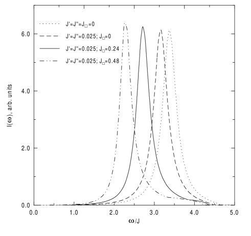
FIG. 1.: Evolution of the two-magnon Raman intensity with increasing ring-exchange couplings; different parameter sets are indicated in the figure.

In Fig. 2 we compare the Raman lineshape, obtained for the parameter set (29) with the experimental data on La₂CuO₄ from Ref. [3]. Although the precise peak position is in excellent agreement with the data, its width is only slightly influenced by ring-exchange coupling. The foot structure near the upper edge of the spectrum does result from ring exchange and therefore indeed leads to an asymmetry of the lineshape, its weight, however, is too small to account for the overall linewidth and lineshape. Therefore, other processes must contribute which are not described by the Heisenberg model with ring exchange alone. It was proposed, that the damping due to spin-phonon coupling [14, 15, 16] is responsible for the peak width which in the current calculation is underestimated by roughly a factor 2. In order to incorporate extrinsic sources for damping beyond the extended Heisenberg Hamiltonian Eq. (1), we have introduced a small damping $\Gamma$ into the denominators of $L_{m}(\omega),$ Eq. (28). As a reasonable choice $\Gamma$ is assumed constant over the entire Brillouin zone, because it is predominantly the zone boundary magnons which determine the shape of the two-magnon peak. We plot the result of this calculation for $\Gamma=0.13J$ in Fig. 2. One can see that while the width of the experimentally observed spectra can be fitted in such a way, the asymmetry of the spectrum is not accounted for. Since the Raman spectra do depend on the incoming light frequency, the two-magnon scattering is identified as a resonant process and therefore an additional source for the strong asymmetry of the lineshape is expected to arise from the coupling to the charge degrees of freedom [17, 18].

In summary, we have investigated the effect of ring exchange on two-magnon Raman scattering in the 2D Heisenberg antiferromagnet. Using the previously fixed exchange coupling parameter set we find in a fit-parameter free calculation an excellent agreement with the position of the two-magnon peak in La₂CuO₄. This reconfirms the magnitude of the ring-exchange coupling $J_{\Box}=0.24J$ in this material. Ring-exchange creates additional high energy spectral weight in the Raman intensity, but $J_{\Box}$ alone is insufficient to explain the overall asymmetric lineshape and linewidth.

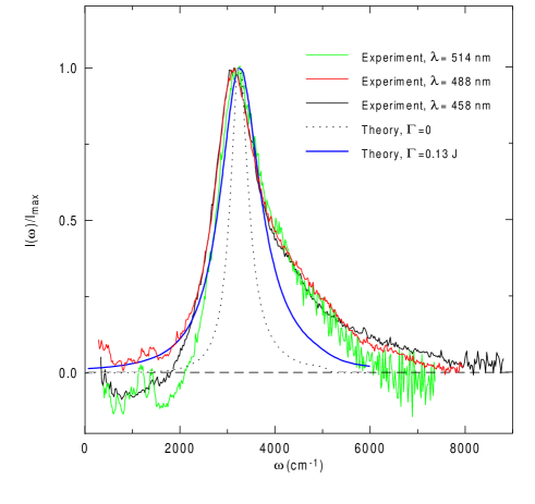
FIG. 2.: Comparison of the theoretical result without ($\Gamma=0$) and with additional damping ($\Gamma=0.13J$) to the experimental Raman intensity in La₂CuO₄ in B_1g geometry taken from Ref. [3]. Calculations were performed with the parameter set (16). The three experimental curves belong to different incoming photon frequencies; the high-energy intensity background was substracted. All data sets were normalized to their corresponding intensity maximum.

It is a pleasure to thank T. Kopp and T. Nunner for insightful discussions. We acknowledge support through Sonderforschungsbereich 484 of the Deutsche Forschungsgemeinschaft.

REFERENCES

[1] E. Manousakis, Rev. Mod. Phys. 63, 1 (1991).
[2] S. Chakravarty, B. I. Halperin, and D. R. Nelson,
Phys. Rev. B 39, 2344 (1989).
[3] K. B. Lyons et al., Phys. Rev. B 39, 9693 (1989); S.
Sugai et al., ibid. 42, 1045 (1990).
[4] J. D. Perkins et al., Phys. Rev. Lett. 71, 1621
(1993).
[5] R. Coldea, S. M. Hayden, G. Aeppli, T. G. Perring, C. D.
Frost, T. E. Mason, S.-W. Cheong, and Z. Fisk, Phys. Rev. Lett. 86,
5377 (2001).
[6] A. A. Katanin and A. P. Kampf, Phys. Rev. B 66,
100403(R) (2002).
[7] E. Müller-Hartmann and A. Reischl, Eur. Phys. J. B 28,
173 (2002).
[8] R. W. Davies, S. R. Chinn, and H. J. Zeiger, Phys. Rev. B
4, 992 (1971).
[9] C. M. Canali and S. M. Girvin, Phys. Rev. B 45, 7127
(1992).
[10] R. R. P. Singh et al., Phys. Rev. Lett. 62, 2736
(1989).
[11] E. Dagotto and D. Poilblanc, Phys. Rev. B 42, 7940
(1990); E. Gagliano and S. Bacci, ibid.42, 8772 (1990).
[12] A.W. Sandvik et al., Phys. Rev. B 57, 8478 (1998).
[13] V. Yu. Irkhin, A. A. Katanin, and M. I. Katsnelson, Phys.
Rev. B 60, 1082 (1999).
[14] P. Knoll et al., Phys. Rev. B42, 4842 (1990).
[15] F. Nori, R. Merlin, S. Haas, A. W. Sandvik, and E. Dagotto,
Phys. Rev. Lett. 75, 553 (1995).
[16] P. J. Freitas and R. R. P. Singh, Phys. Rev. B 62, 5525 (2000).
[17] A. Chubukov and D. Frenkel, Phys. Rev. Lett. 74, 3057 (1995).
[18] F. Schönfeld, A. P. Kampf, and E. Müller-Hartmann,
Z. Phys. B 102, 25 (1997).
[19] C.-M. Ho, V. N. Muthukumar, M. Ogata, and P. W. Anderson,
Phys. Rev. Lett. 86, 1626 (2001).
[20] Y. Honda, Y. Kuramoto, and T. Watanabe, Phys. Rev. B 47, 11329 (1993).
[21] J. Eroles, C. D. Batista, S. B. Bacci, and E. R. Gagliano,
Phys. Rev. B 59, 1468 (1999).
[22] J. Lorenzana, J. Eroles, and S. Sorella, Phys. Rev.
Lett. 83, 5122 (1999).
[23] M. Roger and J. M. Delrieu, Phys. Rev. B 39, 2299
(1989).
[24] M. Takahashi, J. Phys. C: Solid State Phys. 10,
1289 (1977).
[25] A. H. MacDonald, S. M. Girvin, and D. Yoshioka, Phys.
Rev. B 41, 2565 (1990); ibid.37, 9753 (1988).
[26] E. Rastelli and A. Tassi, Phys. Rev. B 11, 4711
(1975).
[27] P. A. Fleury and R. Loudon, Phys. Rev. 166, 514 (1969).