Evidence of a Worldwide Stock Market Log-Periodic Anti-Bubble Since Mid-2000

Abstract

Following our investigation of the USA Standard and Poor index anti-bubble that started in August 2000 [Quantitative Finance 2, 468-481 (2002)], we analyze thirty eight world stock market indices and identify 21 “bearish anti-bubbles” and 6 “bullish anti-bubbles.” An “anti-bubble” is defined as a self-reinforcing price trajectory with self-similar expanding log-periodic oscillations. Mathematically, a “bearish antibubble” is characterize by a power law decrease of the price (or of the logarithm of the price) as a function of time and by expanding log-periodic oscillations. We propose that bearish anti-bubbles are created by positive price-to-price feedbacks feeding overall pessimism and negative market sentiment further strengthened by inter-personal interactions. Bullish anti-bubbles are here identified for the first time. The most striking discovery is that the majority of European and Western stock market indices as well as other stock indices exhibit practically the same log-periodic power law anti-bubble structure as found for the USA S&P500 index. These anti-bubbles are found to start approximately at the same time, August 2000, in all these markets. This shows a remarkable degree of synchronization worldwide. The descent of the worldwide stock markets since 2000 is thus an international event, suggesting the strengthening of globalization.

,

1 Introduction

Financial bubbles are loosely defined as phases of over-valuations of stock market prices above the fundamental prices. Such over-valuations may be in accord with the theory of rational expectations, leading to the concept of rational expectation bubbles [2, 3, 23, 25, 42], may be due to exogenous causes or sunspots (see for instance [5]) or may result from a variety of departures from pure and perfect agent rationality [32, 33, 31, 34, 36].

A series of papers based on analogies with statistical physics models have proposed that most financial crashes are the climax of the so-called log-periodic power law signatures (LPPS) associated with speculative bubbles resulting from imitation between investors and their herding behavior [39, 16, 22, 13, 40]. In addition, a large body of empirical evidence supporting this proposition have been presented [41, 39, 13, 19, 17, 40]. A complementary line of research has established that, while the vast majority of drawdowns occurring on the major financial markets have a distribution which is well-described by an exponential or a slightly fatter distribution in the class of stretched exponentials, the largest drawdowns are occurring with a significantly larger rate than predicted by extrapolating the bulk of the distribution and should thus be considered as outliers [14, 40, 20, 12]. A recent work [21] has merged these two lines of research in a systematic way to offer a classification of crashes as either events of an endogenous origin associated with preceding speculative bubbles or as events of an exogenous origin associated with the markets response to external shocks. Two hallmarks of criticality have been documented: (i) super-exponential power law acceleration of the price towards a “critical” time $t_{c}$ corresponding to the end of the speculative bubble and (ii) log-periodic modulations accelerating according to a geometric series signaling a discrete hierarchy of time scales. Globally over all the markets analyzed, Ref. [21] identified 49 outliers, of which 25 were classified as endogenous, 22 as exogenous and 2 as associated with the Japanese “anti-bubble”. Restricting to the world market indices, Ref. [21] found 31 outliers, of which 19 are endogenous, 10 are exogenous and 2 are associated with the Japanese anti-bubble. The exogenous crashes, not preceded by LPPS could be in each case associated with an important piece of information impacting the market.

All these results taken together formulate a general hypothesis according to which imitation between investors and their herding behavior lead to speculative bubbles of financial markets with accelerating overvaluation decorated by accelerating oscillatory structures possibly followed by crashes or change of regimes. The key concept is the existence of positive price-to-price feedbacks. When speculative prices go up, creating wealth for some investors, this may attract other investors by word-of-mouth interactions, fuelling further price increases. This in turn promotes a wide-spread interest in the media which promotes and amplifies the self-fulfilling wishful thinking [29], with seemingly reasonable or rational theories advanced to justify the price increases. These processes generate more investor demand, fuelling further the expansion of the speculative bubble. The positive price-to-price feedback mechanism has recently been formulated mathematically in a nonlinear generalization of the Black-Scholes stochastic differential equation [37] and in a nonlinear model of stock market prices combining the positive price-to-price feedback with nonlinear negative feedback due to fundamental trading together with inertia [11, 38]. It was there shown that the speculative bubble becomes unstable, reflecting the fact that high prices are ultimately not sustainable, since they are high only because of expectations of further price increases. The bubble eventually bursts, and prices come falling down. The feedback that fed the bubble carries the seeds of its own destruction, and so the end of the bubble and the crash are often unrelated to any really significant news on fundamentals [36].

The same feedback mechanism may also produce a “negative” bubble or “bearish anti-bubble,” that is, downward price movements propelling further downward price movements, enhancing pessimism by inter-personal interactions. Johansen and Sornette [15] proposed indeed that such imitation and herding mechanism may also lead to so-called “anti-bubbles” with decelerating market devaluations following market peaks. The concept of “anti-bubble” was introduced to describe the long-term depression of the Japanese index, the Nikkei, that has decreased along a downward path marked by a succession of ups and downs since its all-time high of 30 Dec. 1989 [15, 18]. The concept of anti-bubble restores a certain degree of symmetry between the speculative behavior of the “bull” and “bear” market regimes. This degree of symmetry, after the critical time $t_{c}$, corresponds to the existence of “anti-bubbles,” characterized by a power law decrease of the price (or of the logarithm of the price) as a function of time $t>t_{c}$, down from a maximum at $t_{c}$ (which is the beginning of the anti-bubble) and by decelerating/expanding log-periodic oscillations [15, 18]. Another anti-bubble was found to describe the gold future prices after its all-time high in 1980. The Russian market prior to and after its speculative peak in 1997 also constitutes a remarkable example where both bubble and anti-bubble structures appear simultaneously for the same $t_{c}$. Several other examples have been described in emergent markets [17].

In a recent paper [43], we have uncovered a remarkable similarity in the behavior of the US S&P500 index from 1996 to August 2002 and of the Japanese Nikkei index from 1985 to 1992 (11 years shift), with particular emphasis on the structure of the bearish phase which is qualified as an anti-bubble according to the previous classification. Specifically, we found the existence of a clear signature of herding in the decay of the S&P500 index since August 2000 with high statistical significance, in the form of strong log-periodic components decorating a power law relaxation.

Here, we show that the (bearish) anti-bubble that started around August 2000 on the USA stock market is actually a world-wide phenomenon with a high degree of correlation and synchronization between most of the western markets. To our knowledge, only during the crash of October 1987 and in its aftermath did stock markets worldwide exhibited a similar or stronger correlation [1, 30].

2 Identification of anti-bubbles in world stock market indexes

2.1 Qualification of an anti-bubble

Following the philosophy of Ref. [21] and references therein (see also [36] for a general review and references therein), we qualify an anti-bubble by the existence of a regime of stock market prices well-fitted by the expression

$$\ln p\left(t\right)\approx A+B\tau^{\alpha}+C\tau^{\alpha}\cos\left[\omega\ln\left(\tau\right)+\phi\right]~{},$$ (1)

which embodies the log-periodic power law signature. Note that the phase $\phi$ does nothing but provide a time scale $T$ since $\omega\ln\left(\tau\right)+\phi=\omega\ln\left(\tau/T\right)$ with the definition $\phi=-\omega\ln T$. $\phi$ thus disappears by the choice of $T$ as the time unit. This stresses the fact that, if the phase is not a fundamental parameter of the fit since it can be get rid of by a suitable gauge choice, it contains nevertheless an important information on the existence of a characteristic time scale. expression (1) obeys the symmetry of discrete scale invariance [35], that has been proposed to be a hallmark of cooperative behavior of interacting agents [22, 13, 36]. The meaning of the adjective “well-fitted” will be clarified below, first by presenting visual evidences in figures and then more formally by statistical tests. For a speculative bubble, we have

$$\tau=t_{c}-t~{},$$ (2)

which is the time to the end of the bubble occurring at $t_{c}$. For an anti-bubble, we have

$$\tau=t-t_{c}~{},$$ (3)

which is the time since the beginning of the anti-bubbles at $t_{c}$. The exponent $\alpha$ should be positive in order for the price $p(t)$ to remain finite at $t=t_{c}$ [13]. In general, speculative bubbles exhibiting the LPPS described by (1) with (2) are followed by crashes or strong corrections that are “outliers” [21]. It may happen that some of these speculative bubbles transform rather into anti-bubbles described by (1) with (3). As we said, this occurred for instance for the Russian speculative bubble ending in 1997. In contrast, anti-bubbles correspond in general to enduring corrections of stock markets that follow a period of strong growth, as exemplified by the trajectory of the Japanese Nikkei index [15, 43] which culminated in Dec. 1989 and then has suffered a non-stop decay decorated by oscillations [15, 18].

Following our previous finding [43] of a strong influence of a log-periodic harmonic at the angular log-frequency $2\omega$ for the S&P500 index, we also present fits including the effect of a harmonic at $2\omega$. In this goal, we postulate the formula

$$\ln p\left(t\right)\approx A+B\tau^{\alpha}+C\tau^{\alpha}\cos\left[\omega\ln\left(\tau\right)+\phi_{1}\right]+D\tau^{\alpha}\cos\left[2\omega\ln\left(\tau\right)+\phi_{2}\right]~{},$$ (4)

which differs from equation (1) by the addition of the last term proportional to the amplitude $D$. The two phases $\phi_{1}$ and $\phi_{2}$ now define two time scales $T_{1}=e^{-\phi_{1}/\omega}$ and $T_{2}=e^{-\phi_{2}/\omega}$. It is thus no longer possible to make them disappear simultaneously by a choice of time unit.

2.2 Methodology

For each stock market described below, we use equations (1) and (4) to fit the logarithm of the stock market indices over an interval starting from a time $t_{\rm start}$ and ending in September, 30, 2002. If we knew the critical time $t_{c}$, then an obvious choice would be $t_{\rm start}=t_{c}$. This choice would be optimal since it allows us to use expression (1) for the longer possible time span compatible with the occurrence of the anti-bubble. Not knowing $t_{c}$ precisely, in order to be consistent with the meaning of expression (1) with (3), we should ensure that $t_{\rm start}\geq t_{c}$.

Furthermore, in accordance with the intuitive meaning of an anti-bubble, we would like to take $t_{\rm start}$ close to the last strong maximum in 2000 and then carry out a sensitivity analysis with respect to $t_{\rm start}$. Fortunately, we shall show that the critical times $t_{c}$ estimated from the fit of the data for different $t_{\rm{start}}$ do not disperse much. In other words, the fits with different $t_{\rm{start}}$ are robust and $t_{c}$ is not very sensitive to $t_{\rm{start}}$. We shall come back to this point later in Sec. 2.6 which will be focused on the best possible characterization of $t_{c}$.

As part of the sensitivity analysis with respect to $t_{\rm start}$, we shall also use the following trick, which ensures that the impact of $t_{\rm start}$ is minimized. Since nothing informs us a priori about the time ordering of $t_{\rm start}$ and $t_{c}$, following [43], we modify expression (3) into

$$\tau=|t-t_{c}|~{}.$$ (5)

This definition (5) has the advantage of removing the constraint of $t_{c}<t_{\rm{start}}$ in the optimization. We see this as an advantage because this constraint has not deep meaning and does not contain any specific information on the data as it results solely from the analyzing procedure and the arbitrary choices for $t_{\rm{start}}$. It thus enables us to test the robustness of fits by scanning different $t_{\rm{start}}$ [43]. Not knowing $t_{c}$ precisely, in order to be consistent with the meaning of expression (1) with (3), we ensure that $t_{\rm start}\geq t_{c}$ by trial and error: a given chosen $t_{\rm start}$ is accepted only if the fit gives a critical time $t_{c}\leq t_{\rm start}$.

While the definition (3) together with the logarithmic as well as power law singularities associated with formula (1) imposes that $t_{c}<t_{\rm start}$ for an anti-bubble, the definition (5) allows for the critical time $t_{c}$ to lie anywhere within the time series. In that case, the part of the time series for $t<t_{c}$ corresponds to an accelerating “bubble” phase while the part $t>t_{c}$ corresponds to a decelerating “anti-bubble” phase. Definition (5) has thus the advantage of introducing a degree of flexibility in the search space for $t_{c}$ without much additional cost. In particular, it allows us to avoid a thorough scanning of $t_{\rm start}$ since the value of $t_{c}$ obtained with this procedure is automatically adjusted without constraint. See Ref. [43] for a discussion of the advantages and potential problems associated with this procedure using (5). Here, we use the definition (5) because it has proved to provide significantly better and more stable fits with little need to vary $t_{\rm start}$.

For a given $t_{\rm start}$, we estimate the parameters $t_{c}$, $\alpha$, $\omega$, $\phi$, $A$, $B$ and $C$ of (1) by minimizing the sum of the squared residues between the fit function (1) and the logarithm of the real index data. Following [22, 13], the three linear parameters $A$, $B$ and $C$ are slaved to the other parameters by solving analytically a system of three linear equations and we are left with optimizing four free parameters. To obtain the global optimization solution, we employ the taboo search [6] to determine an “elite list” of solutions as the initial conditions of the ensuing line search procedures in conjunction with a quasi-Newton method. The best fit thus obtained is regarded to be globally optimized. A similar procedure is used to fit the index with formula (4). This formula has two additional parameters compared with (1), the amplitude $D$ of the harmonic and its phase $\phi_{2}$. We follow a fit procedure which is an adaptation of the slaving method of [22, 13]. This allows us to slave the four parameters $A$, $B$, $C$ and $D$ to the other parameters in the search for the best fit. With this approach, we find that the search of the optimal parameters is very stable and provides fits of very good quality in spite of the remaining five free parameters.

We apply this procedure to 38 stock indices all over the world including:

• eight indices in Americas (Argentina, Brazil, Chile, USA-Dow Jones, Mexico, USA-NASDAQ, Peru, and Veneruela),

• fourteen indices in Asia/Pacific (Australia, China, Hong Kong, India, Indonesia, Japan, Malaysia, New Zealand, Pakistan, Philippines, South Korea, Sri Lanka, Taiwan and Thailand),

• fourteen indices in Europe (Austria, Belgium, Czech, Denmark, France, Germany, Netherlands, Norway, Russia, Slovakia, Spain, Switzerland, Turkey and United Kingdom) and

• two indices in Africa/Middle East (Egypt and Israel).

By the obvious criterion to obtain at least a solution in the fitting procedure, we find no evidence of an anti-bubble in the following eleven indices: Austria, Chile, China, Egypt, Malaysia, New Zealand, Pakistan, Philippines, Slovakia, Sri Lanka and Venezuela. Interestingly, except for Austria and New Zealand, they are emergent markets in developing countries.

The rest of the paper is thus devoted to the study of the remaining 27 indexes out of our initial list of 38.

2.3 Bearish anti-bubbles

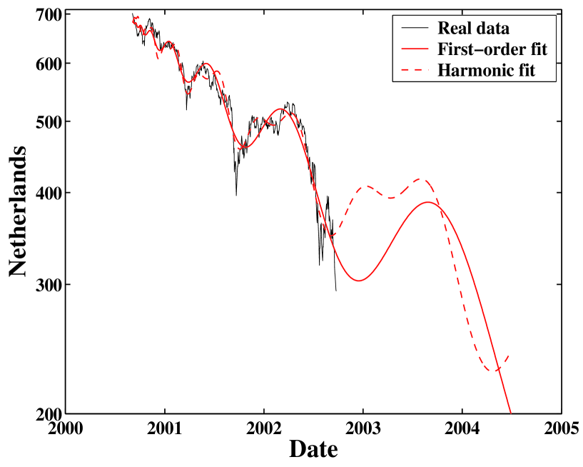
Figure 1: The stock market index of Netherlands (fine noisy line) and its fits with the simple log-periodic formula (1) (thick line) and with formula (4) incorporating an harmonics at $2\omega$ (dashed line). The starting date for the fits is $t_{\rm{start}}=$ 04-Sep-2000 and the ending date of the fit is September, 30, 2002. The parameter values of the fit with (1) are $t_{c}=$ 28-Aug-2000, $\alpha=1.05$, $\omega=9.16$, $\phi=1.63$, $A=6.53$, $B=-0.00055$, and $C=-0.00018$. The r.m.s. of the fit errors is 0.043. The parameter values of the fit with (4) are $t_{c}=$ 20-Jul-2000, $\alpha=0.80$, $\omega=11.07$, $\phi_{1}=4.75$, $\phi_{2}=0.91$, $A=6.60$, $B=-0.00282$, $C=0.00064$, and $D=0.00032$. The r.m.s. of the fit errors is 0.0372. The formula including the harmonics reduces the r.m.s. of fit errors by 13.6%.

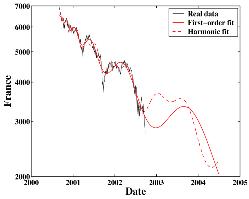
Figure 2: The stock market index of France (fine noisy line) and its fits with the simple log-periodic formula (1) (thick line) and with formula (4) incorporating an harmonics (dashed line). The starting date for the fits is $t_{\rm{start}}=$ 04-Sep-2000. The parameter values of the fit with (1) are $t_{c}=$ 30-Aug-2000, $\alpha=0.92$, $\omega=8.88$, $\phi=3.54$, $A=8.79$, $B=-0.00139$, and $C=-0.00033$. The r.m.s. of the fit errors is 0.0399. The parameter values of the fit with (4) are $t_{c}=$ 04-Jul-2000, $\alpha=0.71$, $\omega=11.24$, $\phi_{1}=0.28$, $\phi_{2}=4.25$, $A=8.90$, $B=-0.00576$, $C=-0.00091$, and $D=0.00048$. The r.m.s. of the fit errors is 0.0347. The formula including the harmonics reduces the r.m.s. of fit errors by 12.9%.

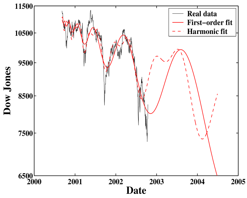
Figure 3: The stock market DowJones index of USA (fine noisy line) and its fits with the simple log-periodic formula (1) (thick line) and with formula (4) incorporating an harmonics (dashed line). The starting date for the fits is $t_{\rm{start}}=$ 06-Sep-2000. The parameter values of the fit with (1) are $t_{c}=$ 15-Aug-2000, $\alpha=1.05$, $\omega=9.76$, $\phi=4.01$, $A=9.30$, $B=-0.00017$, and $C=-0.00011$. The r.m.s. of the fit errors is 0.0337. The parameter values of the fit with (4) are $t_{c}=$ 18-Jun-2000, $\alpha=0.72$, $\omega=12.09$, $\phi_{1}=0.83$, $\phi_{2}=2.16$, $A=9.33$, $B=-0.00145$, $C=-0.00065$, and $D=-0.00034$. The r.m.s. of the fit errors is 0.03. The formula including the harmonics reduces the r.m.s. of fit errors by 11.1%.

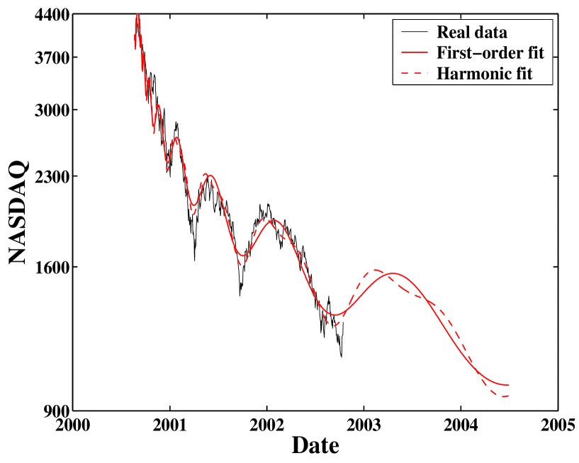
Figure 4: The stock market NASDAQ index of USA (fine noisy line) and its fits with the simple log-periodic formula (1) (thick line) and with formula (4) incorporating an harmonics (dashed line). The starting date for the fits is $t_{\rm{start}}=$ 20-Aug-2000. The parameter values of the fit with (1) are $t_{c}=$ 02-Sep-2000, $\alpha=0.26$, $\omega=10.00$, $\phi=3.37$, $A=8.74$, $B=-0.25128$, and $C=-0.02360$. The r.m.s. of the fit errors is 0.0636. The parameter values of the fit with (4) are $t_{c}=$ 02-Sep-2000, $\alpha=0.26$, $\omega=10.00$, $\phi_{1}=3.37$, $\phi_{2}=0.00$, $A=8.77$, $B=-0.26922$, $C=-0.02473$, and $D=-0.00918$. The r.m.s. of the fit errors is 0.057. The formula including the harmonics reduces the r.m.s. of fit errors by 10.3%.

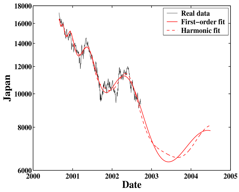
Figure 5: The stock market index of Japan (fine noisy line) and its fits with the simple log-periodic formula (1) (thick line) and with formula (4) incorporating an harmonics (dashed line). The starting date for the fits is $t_{\rm{start}}=$ 28-Aug-2000. The parameter values of the fit with (1) are $t_{c}=$ 06-Aug-2000, $\alpha=0.79$, $\omega=7.74$, $\phi=3.34$, $A=9.74$, $B=-0.00340$, and $C=-0.00086$. The r.m.s. of the fit errors is 0.0396. The parameter values of the fit with (4) are $t_{c}=$ 06-Aug-2000, $\alpha=0.77$, $\omega=7.74$, $\phi_{1}=3.35$, $\phi_{2}=0.00$, $A=9.74$, $B=-0.00372$, $C=-0.00089$, and $D=0.00021$. The r.m.s. of the fit errors is 0.0369. The formula including the harmonics reduces the r.m.s. of fit errors by 6.9%.

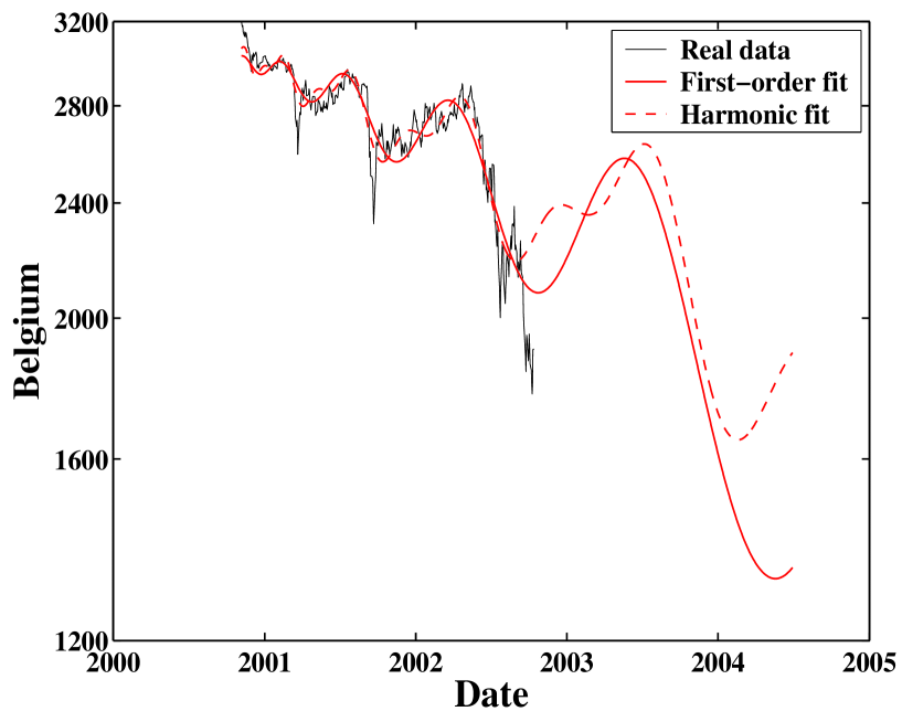
Figure 6: The stock market index of Belgium (fine noisy line) and its fits with the simple log-periodic formula (1) (thick line) and with formula (4) incorporating an harmonics (dashed line). The starting date for the fits is $t_{\rm{start}}=$ 06-Nov-2000. The parameter values of the fit with (1) are $t_{c}=$ 25-Jun-2000, $\alpha=1.52$, $\omega=12.20$, $\phi=2.85$, $A=8.02$, $B=-0.00001$, and $C=0.00000$. The r.m.s. of the fit errors is 0.0336. The parameter values of the fit with (4) are $t_{c}=$ 21-Jun-2000, $\alpha=1.14$, $\omega=12.24$, $\phi_{1}=2.67$, $\phi_{2}=0.49$, $A=8.05$, $B=-0.00012$, $C=0.00005$, and $D=-0.00002$. The r.m.s. of the fit errors is 0.0283. The formula including the harmonics reduces the r.m.s. of fit errors by 15.9%.

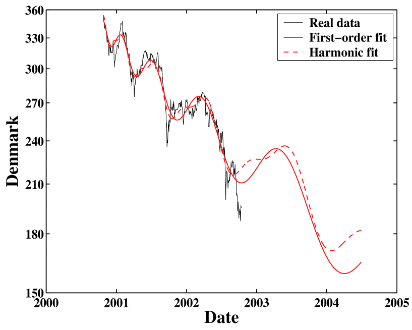
Figure 7: The stock market index of Denmark (fine noisy line) and its fits with the simple log-periodic formula (1) (thick line) and with formula (4) incorporating an harmonics (dashed line). The starting date for the fits is $t_{\rm{start}}=$ 24-Oct-2000. The parameter values of the fit with (1) are $t_{c}=$ 03-May-2000, $\alpha=0.78$, $\omega=13.37$, $\phi=0.62$, $A=5.98$, $B=-0.00273$, and $C=0.00047$. The r.m.s. of the fit errors is 0.0316. The parameter values of the fit with (4) are $t_{c}=$ 04-May-2000, $\alpha=0.64$, $\omega=13.35$, $\phi_{1}=0.87$, $\phi_{2}=0.00$, $A=6.04$, $B=-0.00751$, $C=0.00105$, and $D=0.00036$. The r.m.s. of the fit errors is 0.0286. The formula including the harmonics reduces the r.m.s. of fit errors by 9.6%.

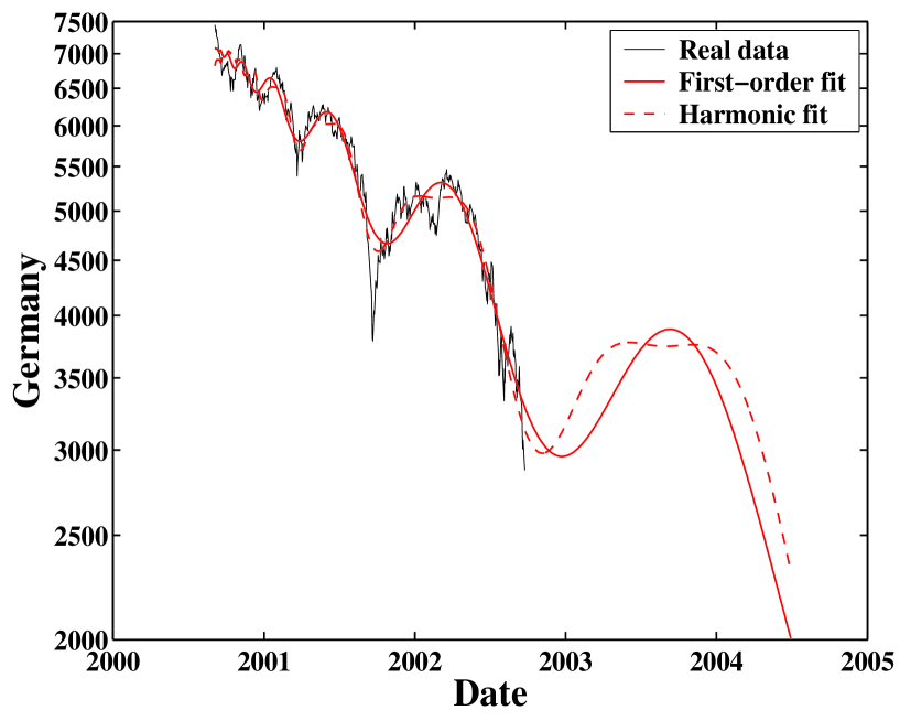
Figure 8: The stock market index of Germany (fine line) and its fits with the simple log-periodic formula (1) (thick line) and with formula (4) incorporating an harmonics (dashed line). The starting date for the fits is $t_{\rm{start}}=$ 04-Sep-2000. The parameter values of the fit with (1) are $t_{c}=$ 31-Aug-2000, $\alpha=1.05$, $\omega=9.02$, $\phi=5.66$, $A=8.87$, $B=-0.00057$, and $C=0.00019$. The r.m.s. of the fit errors is 0.0439. The parameter values of the fit with (4) are $t_{c}=$ 06-Oct-2000, $\alpha=0.94$, $\omega=8.47$, $\phi_{1}=3.61$, $\phi_{2}=4.58$, $A=8.86$, $B=-0.00120$, $C=0.00041$, and $D=0.00012$. The r.m.s. of the fit errors is 0.0396. The formula including the harmonics reduces the r.m.s. of fit errors by 10.0%.

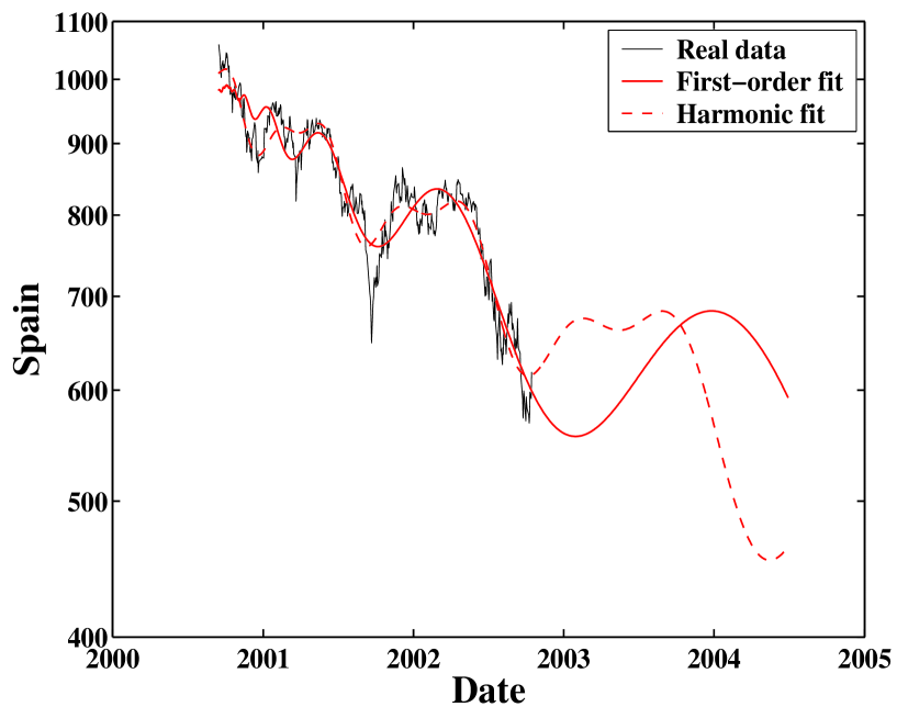
Figure 10: The stock market index of Spain (fine noisy line) and its fits with the simple log-periodic formula (1) (thick line) and with formula (4) incorporating an harmonics (dashed line). The starting date for the fits is $t_{\rm{start}}=$ 14-Sep-2000. The parameter values of the fit with (1) are $t_{c}=$ 04-Oct-2000, $\alpha=0.93$, $\omega=7.52$, $\phi=3.15$, $A=6.90$, $B=-0.00082$, and $C=0.00031$. The r.m.s. of the fit errors is 0.0398. The parameter values of the fit with (4) are $t_{c}=$ 03-Jul-1999, $\alpha=0.88$, $\omega=15.70$, $\phi_{1}=1.75$, $\phi_{2}=1.28$, $A=7.14$, $B=-0.00114$, $C=-0.00018$, and $D=0.00008$. The r.m.s. of the fit errors is 0.0346. The harmonic formula reduces the r.m.s. of fit errors by 12.9%.

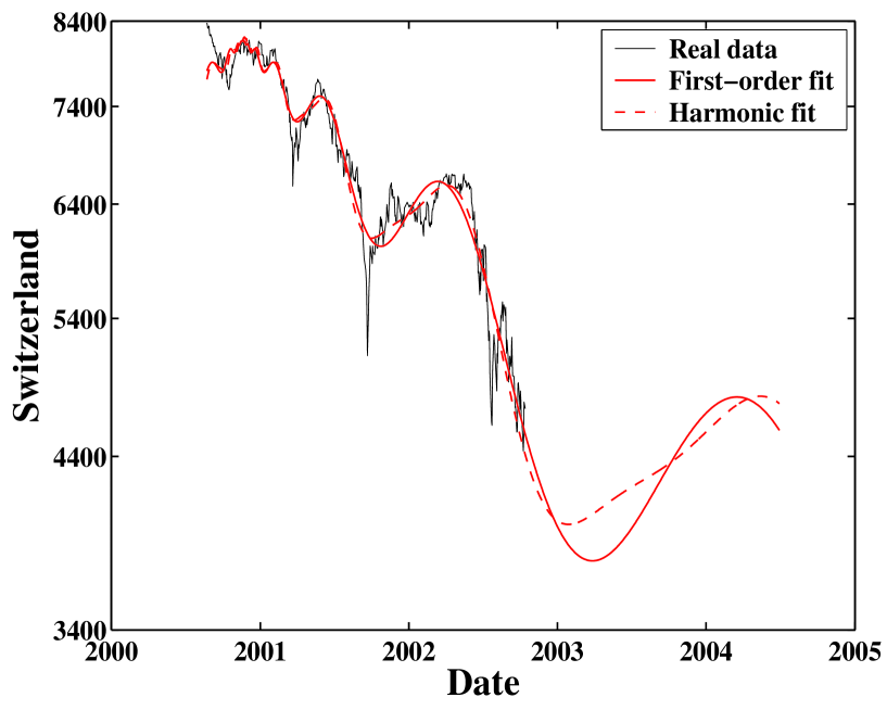
Figure 11: The stock market index of Switzerland (fine noisy line) and its fits with the simple log-periodic formula (1) (thick line) and with formula (4) incorporating an harmonics (dashed line). The starting date for the fits is $t_{\rm{start}}=$ 23-Aug-2000. The parameter values of the fit with (1) are $t_{c}=$ 18-Nov-2000, $\alpha=1.00$, $\omega=6.76$, $\phi=5.16$, $A=9.01$, $B=-0.00070$, and $C=-0.00026$. The r.m.s. of the fit errors is 0.0367. The parameter values of the fit with (4) are $t_{c}=$ 23-Nov-2000, $\alpha=0.95$, $\omega=6.72$, $\phi_{1}=5.54$, $\phi_{2}=0.00$, $A=9.01$, $B=-0.00098$, $C=-0.00035$, and $D=-0.00007$. The r.m.s. of the fit errors is 0.0352. The formula including the harmonics reduces the r.m.s. of fit errors by 4.0%.

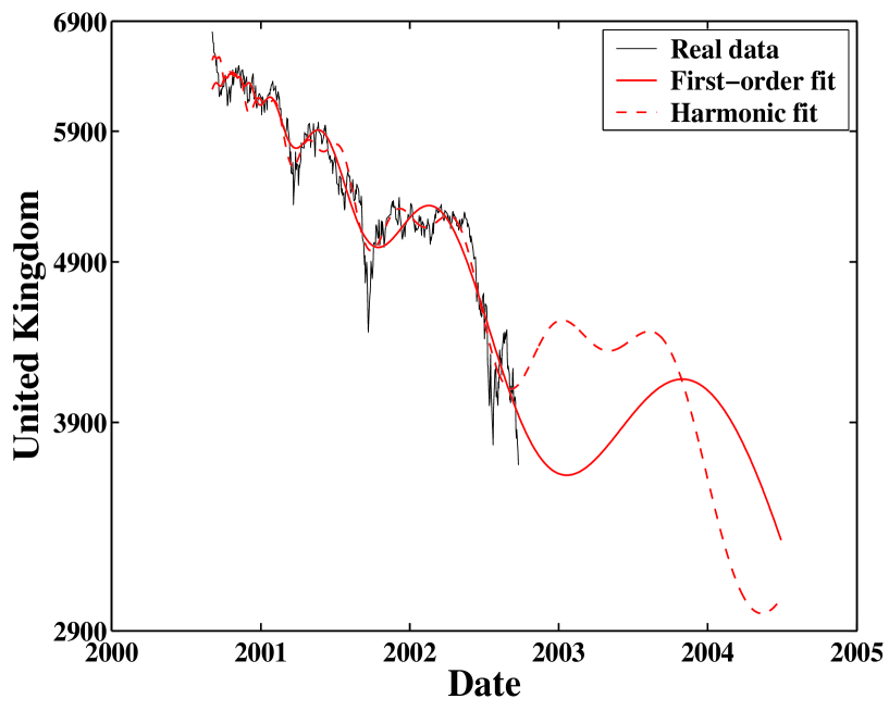
Figure 12: The stock market index of UK (fine noisy line) and its fits with the simple log-periodic formula (1) (thick line) and with formula (4) incorporating an harmonics (dashed line). The starting date for the fits is $t_{\rm{start}}=$ 04-Sep-2000. The parameter values of the fit with (1) are $t_{c}=$ 23-Oct-2000, $\alpha=1.00$, $\omega=7.58$, $\phi=0.00$, $A=8.77$, $B=-0.00055$, and $C=-0.00017$. The r.m.s. of the fit errors is 0.0317. The parameter values of the fit with (4) are $t_{c}=$ 21-Jul-2000, $\alpha=0.84$, $\omega=10.78$, $\phi_{1}=3.56$, $\phi_{2}=1.52$, $A=8.83$, $B=-0.00153$, $C=-0.00030$, and $D=-0.00016$. The r.m.s. of the fit errors is 0.0282. The formula including the harmonics reduces the r.m.s. of fit errors by 11.2%.

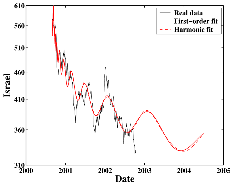
Figure 13: The stock market index of Israel (fine noisy line) and its fits with the simple log-periodic formula (1) (thick line) and with formula (4) incorporating an harmonics (dashed line). The starting date for the fits is $t_{\rm{start}}=$ 28-Aug-2000. The parameter values of the fit with (1) are $t_{c}=$ 09-Sep-2000, $\alpha=0.18$, $\omega=11.45$, $\phi=4.02$, $A=6.61$, $B=-0.20470$, and $C=0.01772$. The r.m.s. of the fit errors is 0.0451. The parameter values of the fit with (4) are $t_{c}=$ 09-Sep-2000, $\alpha=0.19$, $\omega=11.41$, $\phi_{1}=4.26$, $\phi_{2}=0.00$, $A=6.60$, $B=-0.19459$, $C=0.01728$, and $D=-0.00173$. The r.m.s. of the fit errors is 0.0449. The formula including the harmonics reduces the r.m.s. of fit errors by 0.4%.

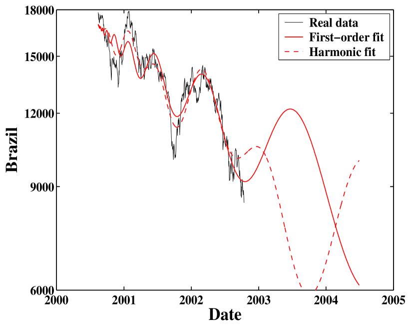
Figure 14: The stock market index of Brazil (fine noisy line) and its fits with the simple log-periodic formula (1) (thick line) and with formula (4) incorporating an harmonics (dashed line). The starting date for the fits is $t_{\rm{start}}=$ 14-Aug-2000. The parameter values of the fit with (1) are $t_{c}=$ 12-Aug-2000, $\alpha=0.87$, $\omega=10.15$, $\phi=4.74$, $A=9.74$, $B=-0.00136$, and $C=0.00056$. The r.m.s. of the fit errors is 0.062. The parameter values of the fit with (4) are $t_{c}=$ 23-Feb-2000, $\alpha=1.08$, $\omega=7.99$, $\phi_{1}=6.24$, $\phi_{2}=4.69$, $A=9.83$, $B=-0.00034$, $C=-0.00007$, and $D=-0.00008$. The r.m.s. of the fit errors is 0.0541. The formula including the harmonics reduces the r.m.s. of fit errors by 12.8%.

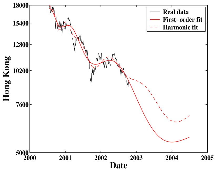
Figure 15: The stock market index of Hong-Kong (fine noisy line) and its fits with the simple log-periodic formula (1) (thick line) and with formula (4) incorporating an harmonics (dashed line). The starting date for the fits is $t_{\rm{start}}=$ 21-Jul-2000. The parameter values of the fit with (1) are $t_{c}=$ 26-Feb-2000, $\alpha=0.90$, $\omega=7.65$, $\phi=1.95$, $A=9.90$, $B=-0.00169$, and $C=-0.00029$. The r.m.s. of the fit errors is 0.0527. The parameter values of the fit with (4) are $t_{c}=$ 30-Jan-2000, $\alpha=0.41$, $\omega=7.52$, $\phi_{1}=2.21$, $\phi_{2}=0.41$, $A=10.39$, $B=-0.07168$, $C=-0.00488$, and $D=0.00303$. The r.m.s. of the fit errors is 0.0463. The formula including the harmonics reduces the r.m.s. of fit errors by 12.2%.

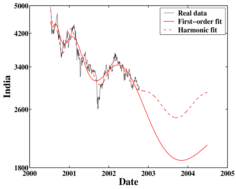
Figure 16: The stock market index of India (fine noisy line) and its fits with the simple log-periodic formula (1) (thick line) and with formula (4) incorporating an harmonics (dashed line). The starting date for the fits is $t_{\rm{start}}=$ 12-Jul-2000. The parameter values of the fit with (1) are $t_{c}=$ 26-May-2000, $\alpha=0.78$, $\omega=6.34$, $\phi=5.61$, $A=8.47$, $B=-0.00292$, and $C=-0.00085$. The r.m.s. of the fit errors is 0.0489. The parameter values of the fit with (4) are $t_{c}=$ 04-Dec-1999, $\alpha=0.03$, $\omega=8.84$, $\phi_{1}=5.96$, $\phi_{2}=0.73$, $A=17.34$, $B=-7.54442$, $C=-0.06297$, and $D=0.03948$. The r.m.s. of the fit errors is 0.0412. The formula including the harmonics reduces the r.m.s. of fit errors by 15.7%.

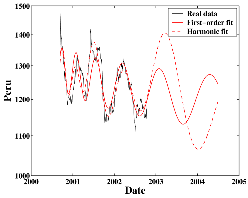
Figure 17: The stock market index of Peru (fine noisy line) and its fits with the simple log-periodic formula (1) (thick line) and with formula (4) incorporating an harmonics (dashed line). The starting date for the fits is $t_{\rm{start}}=$ 11-Sep-2000. The parameter values of the fit with (1) are $t_{c}=$ 28-Oct-1999, $\alpha=0.15$, $\omega=19.80$, $\phi=1.16$, $A=7.45$, $B=-0.11761$, and $C=-0.02090$. The r.m.s. of the fit errors is 0.0322. The parameter values of the fit with (4) are $t_{c}=$ 26-Feb-2000, $\alpha=0.54$, $\omega=7.69$, $\phi_{1}=2.98$, $\phi_{2}=4.99$, $A=7.19$, $B=-0.00167$, $C=0.00120$, and $D=0.00192$. The r.m.s. of the fit errors is 0.0276. The formula including the harmonics reduces the r.m.s. of fit errors by 14.4%.

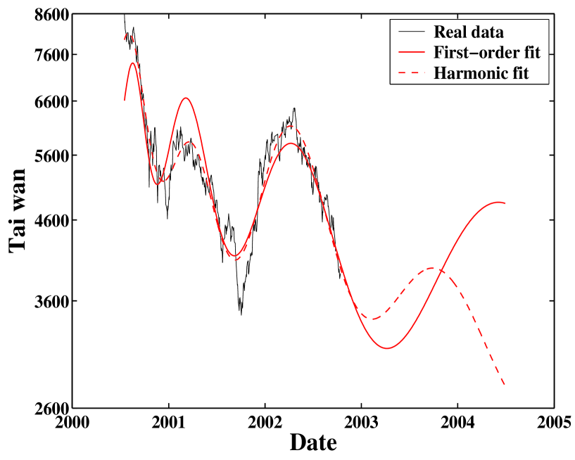
Figure 18: The stock market index of Taiwan (fine noisy line) and its fits with the simple log-periodic formula (1) (thick line) and with formula (4) incorporating an harmonics (dashed line). The starting date for the fits is $t_{\rm{start}}=$ 17-Jul-2000. The parameter values of the fit with (1) are $t_{c}=$ 24-Jan-2000, $\alpha=0.38$, $\omega=9.22$, $\phi=1.01$, $A=9.26$, $B=-0.06302$, and $C=0.01769$. The r.m.s. of the fit errors is 0.085. The parameter values of the fit with (4) are $t_{c}=$ 07-May-1999, $\alpha=0.31$, $\omega=7.34$, $\phi_{1}=1.93$, $\phi_{2}=4.44$, $A=9.95$, $B=-0.18106$, $C=-0.01451$, and $D=0.02150$. The r.m.s. of the fit errors is 0.0541. The formula including the harmonics reduces the r.m.s. of fit errors by 36.3%.

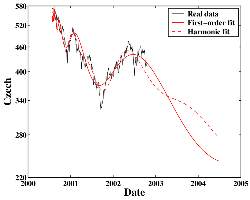
Figure 19: The stock market index of Czech republic (fine noisy line) and its fits with the simple log-periodic formula (1) (thick line) and with formula (4) incorporating an harmonics (dashed line). The starting date for the fits is $t_{\rm{start}}=$ 28-Jul-2000. The parameter values of the fit with (1) are $t_{c}=$ 13-Aug-2000, $\alpha=0.53$, $\omega=4.61$, $\phi=1.19$, $A=6.32$, $B=-0.01246$, and $C=0.00520$. The r.m.s. of the fit errors is 0.048. The parameter values of the fit with (4) are $t_{c}=$ 11-Aug-2000, $\alpha=0.40$, $\omega=4.59$, $\phi_{1}=1.27$, $\phi_{2}=0.77$, $A=6.39$, $B=-0.03390$, $C=0.00969$, and $D=-0.00446$. The r.m.s. of the fit errors is 0.0394. The formula including the harmonics reduces the r.m.s. of fit errors by 17.8%.

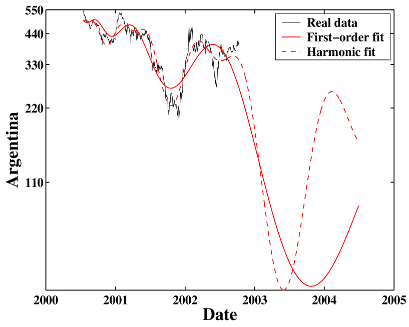
Figure 20: The stock market index of Argentina (fine noisy line) and its fits with the simple log-periodic formula (1) (thick line) and with formula (4) incorporating an harmonics (dashed line). The starting date for the fits is $t_{\rm{start}}=$ 14-Jul-2000. The parameter values of the fit with (1) are $t_{c}=$ 02-May-2000, $\alpha=1.54$, $\omega=7.25$, $\phi=5.28$, $A=6.23$, $B=-0.00003$, and $C=-0.00002$. The r.m.s. of the fit errors is 0.1223. The parameter values of the fit with (4) are $t_{c}=$ 23-Aug-1999, $\alpha=2.00$, $\omega=11.23$, $\phi_{1}=0.67$, $\phi_{2}=4.40$, $A=6.25$, $B=-0.00000$, $C=-0.00000$, and $D=0.00000$. The r.m.s. of the fit errors is 0.082. The formula including the harmonics reduces the r.m.s. of fit errors by 32.9%.

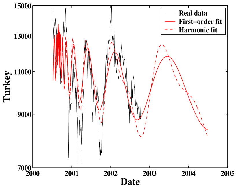
Figure 21: The stock market index of Turkey (fine noisy line) and its fits with the simple log-periodic formula (1) (thick line) and with formula (4) incorporating an harmonics (dashed line). The starting date for the fits is $t_{\rm{start}}=$ 10-Jul-2000. The parameter values of the fit with (1) are $t_{c}=$ 28-Aug-2000, $\alpha=0.13$, $\omega=9.56$, $\phi=2.88$, $A=9.62$, $B=-0.16041$, and $C=0.06365$. The r.m.s. of the fit errors is 0.1176. The parameter values of the fit with (4) are $t_{c}=$ 28-Aug-2000, $\alpha=0.20$, $\omega=9.55$, $\phi_{1}=2.94$, $\phi_{2}=1.32$, $A=9.52$, $B=-0.07816$, $C=0.04712$, and $D=0.01847$. The r.m.s. of the fit errors is 0.1104. The formula including the harmonics reduces the r.m.s. of fit errors by 6.1%.

Anti-bubbles are identified in 21 stock market indices: Netherlands, France, USA Dow Jones, USA NASDAQ, Japan, Belgium, Denmark, Germany, Norway, Spain, Switzerland, United Kingdom, Israel, Brazil, Hong Kong, India, Peru, Taiwan, Czech, Argentina and Turkey. We refer to these anti-bubble by the term “bearish” to stress that they are fitted by an overall decreasing power law (since $B<0$ and $\alpha>0$). Figures 1-21 present the fits of these 21 bearish anti-bubbles by expression (1) and (4). The corresponding parameters are listed in Tables 1 and 2. Similar bearish anti-bubbles were observed before in Latin-American, Asian and Western Stock markets [15, 17]. We also show the extrapolation of these fits by formulas (1) and (4) until mid-2004, in the spirit of the analysis presented for the USA S&P500 index [43].

These figures show that the log-periodic structures are very prominent. For instance, four to five log-periodic oscillations can be identified for most of the cases presented. However, for some indices, the log-periodic oscillations close to $t_{c}$ are strongly affected by noise for some indices and are less clear-cut.

The majority of predicted critical times $t_{c}$ for the launch of the anti-bubbles fall between August and November, 2000: eight in August, two in September, three in October and one in November. This is in agreement with the determination $t_{c}=$ Aug-09-2000 for the S&P500 index [43], suggesting a worldwide synchronization of the start of a bearish anti-bubble phase.

This analysis, paralleling that presented for the USA S&P500 index [43], suggests that many of the stock markets shown here are in a phase of recovery that started close to the last date, September 30, 2002, used to perform the fit. This recovery is predicted by the extrapolations of (1) and (4) to extend until some time in 2003 depending upon the markets (see the figures) before a recession resumes for a while. However, we do not claim that these extrapolations should be valid beyond roughly the end of 2003. The statement applies to the markets of The Netherlands, France, USA (Dow Jones and NASDAQ), Belgium, Denmark, Germany, Norway, Spain, Israel, Peru, and Turkey. We note also that there is sometimes a substantial difference between the timing of the recovery and the following recession predicted by expression (1) compared with formula (4). This is the case for the stock markets of the Netherlands, France, the USA Dow Jones, Norway, Spain, and the United Kingdom. In these cases, one should be careful in interpreting these extrapolations as reliable forecasts. In some cases, such as for the United Kingdom and Brazil, the two extrapolations are so inconsistent as being meaningless. Thus, our message here is not so much the forecasts but instead the remarkable consistency in the log-periodicity of these anti-bubble phases, shown by their common starting dates and similar structures quantified by the power law exponents and the angular log-frequencies.

In contrast, the markets of Japan, Switzerland, Hong Kong, India, Taiwan, Czech and Argentina are extrapolated to continue their overall descent roughly till the middle of 2003 or beyond before a recovery sets in. The clear log-periodic structure since August 2000 shown in figure 5 for the Japanese Nikkei index is especially interesting because this structure follows the large scale anti-bubble log-periodic pattern that started in January 1990 [15] and continued at least until the beginning of 2000 [18]. A possible interpretation of the novel structure identified in figure 5 is that it is a sub-structure within a hierarchy of log-periodic patterns occurring at many different scales, as found for instance in Weierstrass functions (see [8] for an interpretation of Weierstrass functions and their generalizations in terms of log-periodicity at many different scales) and suggested in [7]. We can expect more generally that similar multiscale log-periodicity should exist in other markets. However, these fine structures especially at the smaller scales (three months, monthly, weekly, intraday, etc.) are greatly effected or even spoiled by the intrinsically noisy nature of stock market prices, due to the fact that many more effects contribute potentially at small scales to scramble possible signals. Only at the large time scales studied here can the cooperative behavior of investors be systematically observed.

Another important observation is that the log-periodic oscillations and power law decays are distinctly different with a smaller number of oscillations and much larger “noise” for Brazil, Hong-Kong, India, Peru, Taiwan, Czech republic, Argentina and Turkey compared with the others. This may be explained by the presence of stronger idiosyncratic influences, such as local crises in South America. For these markets, the two extrapolations obtained from expressions (1) and (4) diverge rapidly away from each other, making them quite unreliable.

As shown in Table 1, the power law exponents $\alpha$ of the indices of Belgium and Argentina are significantly larger than $1$, while those of Netherland, USA Dow Jones, Germany, Norway, Switzerland and United Kingdom are close to or slightly greater than $1$. In absence of the log-periodic oscillations, this would mean that the overall shape of these indices would be concave (downward plunging) rather than convex (upward curvature) as they would be for $0<\alpha<1$. Large values of $\alpha>1$ implies a steep downward overall acceleration of the index. But in all cases when this occurs, this is compensated by a large amplitude of the log-periodic oscillations. In contrast, for $0<\alpha<1$, the index initially drops fast in the early times of the anti-bubble and then decelerates and approaches a constant level at long times.

To quantify the significance level of the log-periodic oscillations in these 21 anti-bubbles, we adopt the Lomb analysis [26] on the residuals of the logarithm of the indices by removing the power law [17]:

$$r(t)={\ln p(t)-A-B\tau^{\alpha}\over C\tau^{\alpha}},$$ (6)

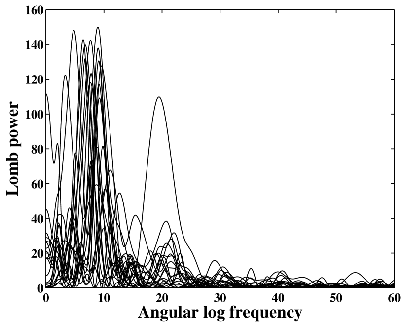
Figure 22: Lomb periodograms for the 21 stock market indices shown in previous figures as a function of the angular log-periodic frequency $\omega$. These 21 stock market indices exhibit a so-called bearish anti-bubble regime characterized by $B<0$. The number of points in the Lomb analysis is in the range 350-530, which implies that the log-periodic signals are very significant for most markets with high Lomb peaks. The relevance of the log-periodicity is reflected in the quasi-universal value of the angular log-periodic frequency found in the range $7-10$. Notice also the presence of an harmonic at $2\omega$ in many of the markets outlined by the cluster of secondary peaks in the vicinity of $\omega=20$.

where $\tau$ is defined in (3). If the log-periodic formula is a correct representation of these indices, $r(t)$ should be a pure cosine as a function of $\ln\tau$. Thus, a spectral analysis of $r(t)$ as a function of the variable $\ln\tau$ should be a strong power peak. Figure 22 presents the corresponding Lomb periodograms for all 21 indices described in table 1 and shown in figures 1-21. Most of the Lomb spectral peaks give a very significant signal of the existence of log-periodic structures [44].

In addition, an harmonic of a fundamental angular log-frequency $\omega$ is visible at $2\omega$ in the Lomb periodogram for many of the markets, as found previously for the S&P 500 index [43]. This is the justification for including an harmonic log-periodic oscillatory term according to (4). Table 2 lists the corresponding parameters of the fits of the 21 stock market indices with expression (4) and shows that using of formula (4) reduces the r.m.s. errors strongly for most of the indexes. Only for Israel is the improvement of the fit ambiguous. In section 2.5, we shall come back to this issue and provide rigorous and objective statistical tests on the relevance of log-periodicity with a single angular log-frequency $\omega$ and with the addition of its harmonics at $2\omega$.

2.4 Bullish anti-bubbles

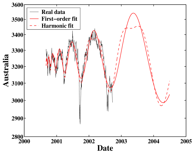
Figure 23: The stock market index of Australia (fine line) and its fits with the simple log-periodic formula (1) (thick line) and with formula (4) incorporating an harmonics (dashed line). The starting date for the fits is $t_{\rm{start}}=$ 04-Sep-2000 and the ending date of the fit is September, 30, 2002. The parameter values of the fit with (1) are $t_{c}=$ 08-Aug-2000, $\alpha=0.77$, $\omega=10.85$, $\phi=3.55$, $A=8.08$, $B=0.00007$, and $C=-0.00037$. The r.m.s. of the fit errors is 0.0176. The parameter values of the fit with (4) are $t_{c}=$ 10-Aug-2000, $\alpha=0.64$, $\omega=10.89$, $\phi_{1}=3.42$, $\phi_{2}=0.51$, $A=8.08$, $B=0.00026$, $C=-0.00080$, and $D=-0.00026$. The r.m.s. of the fit errors is 0.0153. The formula including the harmonics reduces the r.m.s. of fit errors by 13.2%.

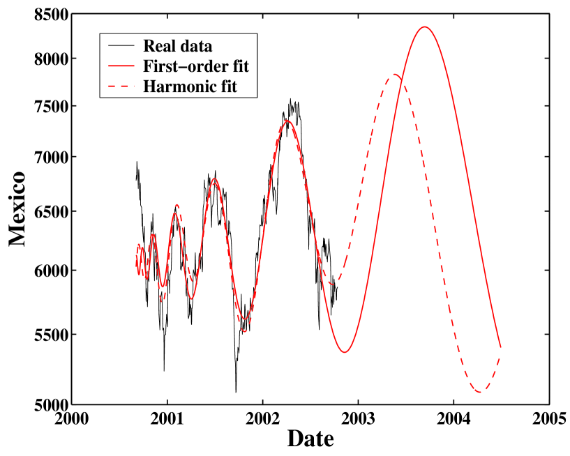
Figure 24: The stock market index of Mexico (fine line) and its fits with the simple log-periodic formula (1) (thick line) and with formula (4) incorporating an harmonics (dashed line). The starting date for the fits is $t_{\rm{start}}=$ 04-Sep-2000. The parameter values of the fit with (1) are $t_{c}=$ 08-Aug-2000, $\alpha=0.80$, $\omega=10.11$, $\phi=4.42$, $A=8.70$, $B=0.00032$, and $C=0.00086$. The r.m.s. of the fit errors is 0.0402. The parameter values of the fit with (4) are $t_{c}=$ 27-Jun-2000, $\alpha=0.73$, $\omega=5.97$, $\phi_{1}=4.23$, $\phi_{2}=1.65$, $A=8.69$, $B=0.00072$, $C=0.00039$, and $D=-0.00115$. The r.m.s. of the fit errors is 0.0391. The formula including the harmonics reduces the r.m.s. of fit errors by 2.6%.

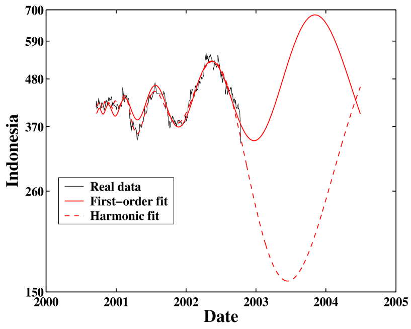
Figure 25: The stock market index of Indonesia (fine line) and its fits with the simple log-periodic formula (1) (thick line) and with formula (4) incorporating an harmonics (dashed line). The starting date for the fits is $t_{\rm{start}}=$ 16-Sep-2000. The parameter values of the fit with (1) are $t_{c}=$ 09-Aug-2000, $\alpha=1.06$, $\omega=10.30$, $\phi=5.83$, $A=5.99$, $B=0.00009$, and $C=-0.00021$. The r.m.s. of the fit errors is 0.039. The parameter values of the fit with (4) are $t_{c}=$ 16-Nov-2000, $\alpha=0.96$, $\omega=3.47$, $\phi_{1}=1.33$, $\phi_{2}=3.10$, $A=6.04$, $B=-0.00025$, $C=-0.00050$, and $D=-0.00062$. The r.m.s. of the fit errors is 0.0271. The formula including the harmonics reduces the r.m.s. of fit errors by 30.4%.

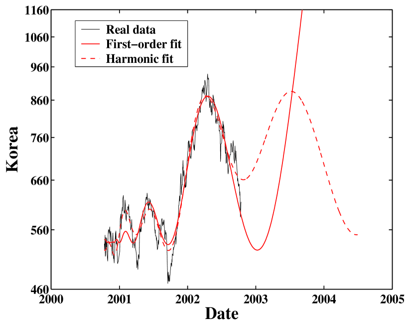
Figure 26: The stock market index of Korea (fine line) and its fits with the simple log-periodic formula (1) (thick line) and with formula (4) incorporating an harmonics (dashed line). The starting date for the fits is $t_{\rm{start}}=$ 12-Oct-2000. The parameter values of the fit with (1) are $t_{c}=$ 15-Nov-2000, $\alpha=1.37$, $\omega=6.69$, $\phi=5.67$, $A=6.29$, $B=0.00005$, and $C=-0.00005$. The r.m.s. of the fit errors is 0.05. The parameter values of the fit with (4) are $t_{c}=$ 10-Aug-2000, $\alpha=1.00$, $\omega=5.04$, $\phi_{1}=1.90$, $\phi_{2}=1.90$, $A=6.24$, $B=0.00046$, $C=-0.00023$, and $D=-0.00025$. The r.m.s. of the fit errors is 0.0428. The formula including the harmonics reduces the r.m.s. of fit errors by 14.4%.

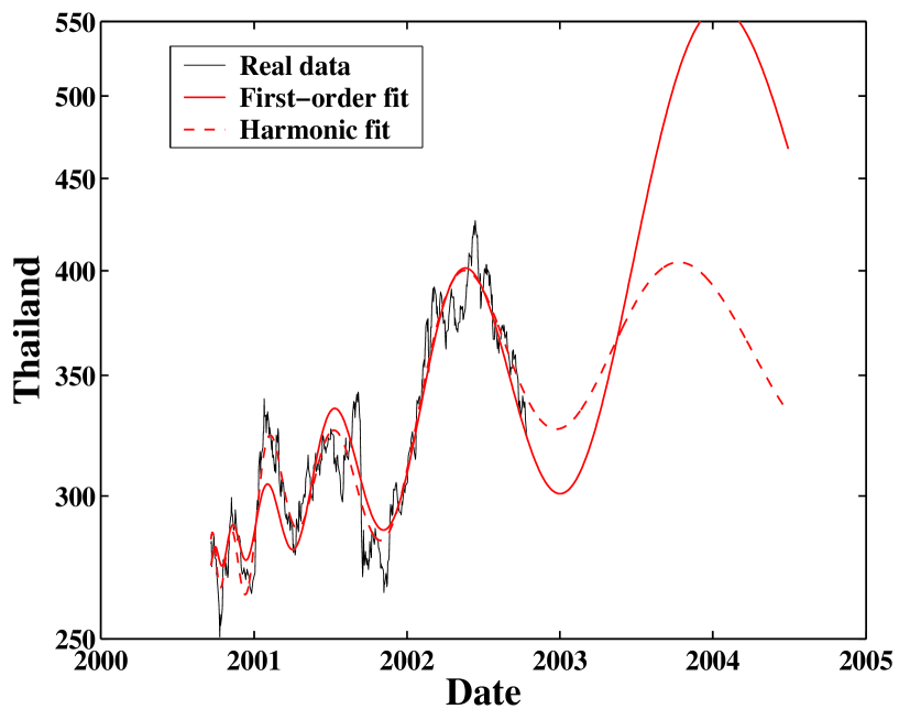
Figure 27: The stock market index of Thailand (fine line) and its fits with the simple log-periodic formula (1) (thick line) and with formula (4) incorporating an harmonics (dashed line). The starting date for the fits is $t_{\rm{start}}=$ 20-Sep-2000. The parameter values of the fit with (1) are $t_{c}=$ 16-Aug-2000, $\alpha=0.93$, $\omega=9.45$, $\phi=5.16$, $A=5.61$, $B=0.00058$, and $C=-0.00039$. The r.m.s. of the fit errors is 0.0437. The parameter values of the fit with (4) are $t_{c}=$ 27-Jul-2000, $\alpha=0.43$, $\omega=5.18$, $\phi_{1}=3.62$, $\phi_{2}=2.22$, $A=5.48$, $B=0.02083$, $C=0.00390$, and $D=0.00662$. The r.m.s. of the fit errors is 0.0354. The formula including the harmonics reduces the r.m.s. of fit errors by 19.0%.

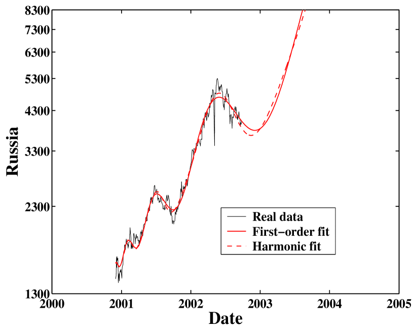
Figure 28: The stock market index of Russia (fine line) and its fits with the simple log-periodic formula (1) (thick line) and with formula (4) incorporating an harmonics (dashed line). The starting date for the fits is $t_{\rm{start}}=$ 01-Dec-2000. The parameter values of the fit with (1) are $t_{c}=$ 08-Oct-2000, $\alpha=0.92$, $\omega=7.93$, $\phi=3.33$, $A=7.24$, $B=0.00276$, and $C=-0.00068$. The r.m.s. of the fit errors is 0.0485. The parameter values of the fit with (4) are $t_{c}=$ 12-Oct-2000, $\alpha=0.91$, $\omega=7.85$, $\phi_{1}=3.90$, $\phi_{2}=0.17$, $A=7.23$, $B=0.00307$, $C=-0.00075$, and $D=0.00010$. The r.m.s. of the fit errors is 0.0457. The formula including the harmonics reduces the r.m.s. of fit errors by 5.7%.

Figures 23-28 present the fits of six stock market indices (Australia, Mexico, Indonesia, South Korea, Thailand and Russia) using formula (1) and (4), with the corresponding parameters listed in Table 3. We have separated these 6 markets from the 21 previous ones because their fits with formulas (1) and (4) give a positive coefficient $B$, corresponding to an overall increasing market at large time scales. We thus call them “bullish” to describe this overall increasing pattern. We keep the terminology “anti-bubble” to refer to the fact that the log-periodic oscillations are decelerating. To the best of our knowledge, the identification of such bullish anti-bubbles is performed here for the first time. Notice that there are five log-periodic oscillations for Australia, Indonesia and Thailand, four for and Mexico and approximately three for South Korea and Russia as can be seen in the figures 23-28. This means that the log-periodic structures in these stock market indices are quite significant and convincing [44]. Table 3 shows that the predicted critical times $t_{c}$ of the start of these bullish anti-bubbles are again between August and November, 2000.

We have also performed a fit of these 6 stock market indices with expression (4) which accounts for the possible presence of an harmonic log-periodic oscillatory term. The fits are plotted in Figs. 23-28 as dashed lines, whose parameters are presented in Table 4. We find that the improvement of the fits using expression (4) compared with (1) is very significant for Australia, Korea, Indonesia and Thailand.

2.5 Statistical test of the log-periodic term

Since expression (4) contains formula (1) as the special case $D=0$, we can use Wilk’s theorem [28] and the statistical methodology of nested hypotheses to assess whether the hypothesis that $D=0$ can be rejected. Similarly, we can also test if $C=0$ can be rejected in (1). We consider the following three hypotheses.

1. $H_{0}$: $C=0$, corresponding to use a simple and pure power law to fit the stock market indices;

2. $H_{1}$: $D=0$, corresponding to the log-periodic function (1) without any harmonics;

3. $H_{2}$: $D\neq 0$, corresponding to the log-periodic function (4) which includes an harmonics at $2\omega$.

Our tests presented below show that $H_{0}$ can be rejected with certainty in favor of $H_{1}$ for all the indexes which have been analyzed. Moreover, we find that $H_{1}$ can be rejected in favor of $H_{2}$ with high statistical significance for all except one index (rejection level of $10^{-4}\%$). We stress that Wilk’s methodology of nested hypothesis testing automatically takes into account the competition between (i) the improved fit obtained by adding fitting parameters and the “cost in parsimony” of adding these parameters.

The method proceeds as follows (see [40, 43] for recent implementations in similar contexts). Assuming a Gaussian distribution of observational errors (residuals) at each data point, the maximum likelihood estimation of the parameters amounts exactly to the minimization of the sum of the square over all data points (of number $n$) of the differences $\delta_{j}(i)$ between the mathematical formula and the data [26]. The standard deviation $\sigma_{j}$ for hypothesis $H_{j}$ with $j=0,1,2$ of the fits to the data associated with (1) and (4) is given by $1/n$ times the sum of the squares over all data points of the differences $\delta_{j}^{(o)}(i)$ between the mathematical formula and the data, estimated for the optimal parameters of the fit. The log-likelihoods corresponding to the three hypotheses are thus given by

$$L_{j}=-n\ln\sqrt{2\pi}-n\ln\sigma_{j}-n/2~{},$$ (7)

where the third term results from the product of Gaussians in the likelihood, which is of the form

$$\propto\prod_{i=1}^{n}\exp[-(\delta_{j}^{(o)}(i))^{2}/2\sigma_{j}^{2}]=\exp[-n/2]~{},$$

from the definition $\sigma_{j}^{2}=(1/n)\sum_{i=1}^{n}[\delta_{j}^{(o)}(i)]^{2}$. Then, according to Wilk’s theorem of nested hypotheses, the log-likelihood-ratio

$$T_{j,j+1}=-2(L_{j}-L_{j+1})=2n(\ln\sigma_{j}-\ln\sigma_{j+1})~{},~{}~{}~{}j=0,1~{}~{}~{}~{}$$ (8)

is a chi-square variable with $k$ degrees of freedom, where $k$ is the number of restricted parameters [10]. In the present case, we have $k=1$.

The Wilk test thus amounts to calculating the probability $P_{j,j+1}$ that the obtained value of $T_{j,j+1}$ can be overpassed by chance alone. If this probability $P_{j,j+1}$ is small, this means that chance is not a convincing explanation for the large value of $T_{j,j+1}$ which becomes meaningful. This implies a rejection of the hypothesis that $C=0$ (resp. $D=0$) is sufficient to explain the data and favor the fit with $C\neq 0$ (resp. $D\neq 0$) as statistically significant. In other words, if the observed value of the probability $1-P_{j,j+1}$ that $T_{0,1}$ (respectively of $T_{1,2}$) does not exceed some high-confidence level (say, the $99\%$ confidence level) of the $\chi^{2}$, we then reject the hypothesis $H_{1}$ (respectively $H_{2}$) in favor of the hypothesis $H_{0}$ (respectively $H_{1}$), considering the additional term $C$ (respectively $D$) redundant. Otherwise, we accept the hypothesis $H_{1}$ (respectively $H_{2}$, considering the description with $H_{0}$ (respectively $H_{1}$) insufficient.

For each stock index, we fit the corresponding time series starting from $t_{\rm{start}}$ and ending on September 30, 2002 to a simple power law, to the log-periodic function (1) and to the formula (4) respectively, and thus obtain $\sigma_{0}$, $\sigma_{1}$ and $\sigma_{2}$. Then we can calculate $T_{j,j+1}$ from (8) and the corresponding probabilities $P_{j,j+1}$. The results of the Wilk tests are presented in Table 5. The values $T_{0,1}$ are extremely large for all indices, which reject with extremely high statistical significance the hypothesis that a pure power law is sufficient compared to a log-periodic power law. For the test of $H_{2}$ against $H_{1}$, $T_{1,2}$ is found very large ($>40$) for most of the indices, except for Israel ($T_{1,2}=2.7$) and Mexico ($T_{1,2}=25.9$). Even in the case of Mexico, the improvement obtained by adding a the harmonic term (hypothesis $H_{2}$) is nevertheless very significant since $T_{1,2}=25.9$ corresponds to a probability of rejection of $H_{2}$ $P_{1,2}$ less than $10^{-4}\%$. Thus, only for Israel, we find that $D=0$ can not be rejected at the confidence level of $95\%$. This reflect the fact that the reduction of the r.m.s. errors when going from formula (1) to (4) is less that $1\%$. The lack of significant improvement can also be seen visually in Fig. 13.

Since the assumption of Gaussian noise is most probably an under-estimation of the real distribution of noise amplitudes, the very significant improvement in the quality of the fit brought by the use of both formulas (1) and (4) quantified in Table 5 provides most probably a lower bound for the statistical significance of the hypothesis that both $C$ and $D$ should be chosen non-zero, above the $99.9999\%$ confidence level. Indeed, a non-Gaussian noise with a fat-tailed distribution would be expected to decrease the relevance of competing formulas, whose performance could be scrambled and be made fuzzy. The clear and strong result of the Wilk tests with assumed Gaussian noises thus confirm a very strong significance of both formulas (1) and (4).

2.6 Determination of $t_{c}$

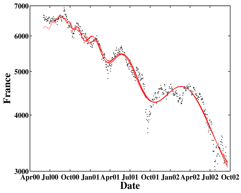
Figure 29: The French stock index, a bearish anti-bubble, fitted from $t_{\rm start}$ to September 2002 for different choices of $t_{\rm start}$, spanning from Jun-01-2000 to Dec-01-2000. One see that the fits are robust with respect to different starting date.

The critical time $t_{c}$ defines the real starting time of the anti-bubbles and is an important parameter for quantifying the synchronization between different stock markets. It is thus important to investigate how robust is its determination by our fitting procedure. In this section, we discuss two markets to illustrate the typical situation, the French stock index as an example of a bearish anti-bubble and the Australia stock index as an example of a bullish anti-bubble. To test for the robustness of the determination of $t_{c}$, we follow the analysis of [43] on the USA Standard and Poor index and take seven different values for $t_{\rm{start}}$ from Jun-01-2000 to Dec-01-2000 for each index. Figure 29 shows the seven best fits, one for each $t_{\rm{start}}$, for the French stock index. The corresponding fitting parameters are listed in Table 6. Three fits in Fig. 29 are slightly different from the rest especially in the early days of the anti-bubble. The starting dates of these three fits are Oct-01-2000, Nov-01-2000 and Dec-01-2000. The slightly different nature of these three cases is also reflected in discernable variations in the fitting parameters listed in Table 6. In particular, they identify a critical $t_{c}$ at the end of October, 2000 rather than mid-August, 2000. They also have slightly larger exponents $\alpha$, lower log-frequencies $\omega$ and smaller $A$. Despite these differences, all the fits are quite robust indicating a critical time at or slightly after August, 2000.

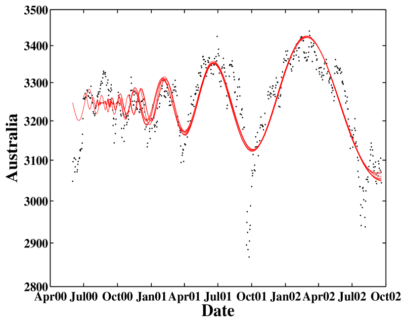
Figure 30: The Australian stock index, a bearish anti-bubble, fitted from $t_{\rm start}$ to September 2002 for different choices of $t_{\rm start}$, spanning from Jun-01-2000 to Dec-01-2000. One see that the fits are robust with respect to different starting date.

Figure 30 shows the seven best fits, one for each $t_{\rm{start}}$, for the Australian stock index. The relevant parameters are listed in Table 7. We also observe three fits starting on Jun-01-2000, Nov-01-2000 and Dec-01-2000 that have relatively later predicted $t_{c}$, slightly larger exponents $\alpha$, lower log-frequencies $\omega$. But the predicted index value at $t_{c}$ (i.e., $e^{A}$) are almost the same. The critical time $t_{c}$ of the Australian anti-bubble is also clustered around mid-August, 2000. This is consistent with the fact that both including extra data earlier than $t_{c}$ ($t_{\rm{start}}\ll t_{c}$) and truncating data after $t_{c}$ ($t_{\rm{start}}\gg t_{c}$) will reduce the precision of the determination of $t_{c}$ and deteriorate the quality of fits.

We nevertheless have to note that not all the indices give such robust results. The log-periodic oscillations in the initial days of some anti-bubbles are completely spoiled by noise, where different effects overwhelm the herding behavior thought to be at the origin of the log-periodic power law patterns. For instance, the existence of an anti-bubble in the Peruvian stock index is quite questionable in view of the particularities in its fitting parameters.

3 Correlation across different markets and synchronization of the anti-bubbles

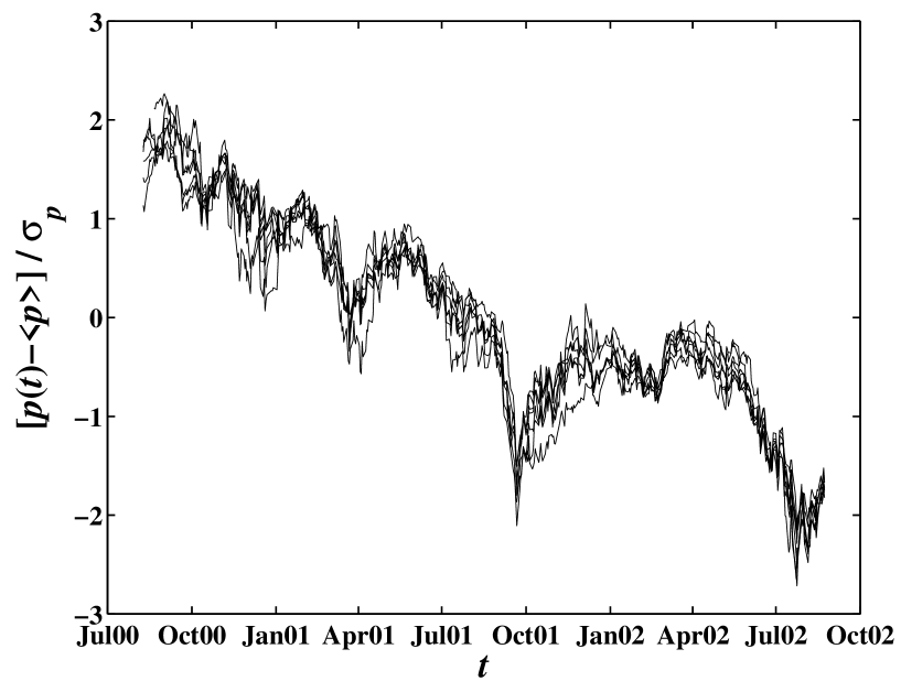
Figure 31: The stock market indices of seven countries (US S&P 500, the Netherlands, France, Germany, Norway, UK, Spain) are superimposed by plotting the normalized values $[p(t)-\langle p\rangle]/\sigma_{p}$ of each index as a function of time, where $\langle p\rangle$ is the mean whose substraction accounts for a country-specific translation in price and $\sigma_{p}$ is the standard deviation for each index which accounts for a country-specific adjustment of scale.

One of the most remarkable results obtained so far is that most of the anti-bubbles started between August and November, 2000, with very similar time evolutions as quantified by the formulas (1) and (4) and by the Tables 1 and 2. This suggests that the triggering of almost simultaneously occurring anti-bubbles is an international event. Figure 31 summarizes our main message by superimposing the stock market indices of seven countries (US S&P 500, the Netherlands, France, Germany, Norway, UK, Spain). The ordinate plots the normalized values $[p(t)-\langle p\rangle]/\sigma_{p}$ of each index as a function of time, where $\langle p\rangle$ is the mean whose substraction accounts for a country-specific translation in price and $\sigma_{p}$ is the standard deviation for each index which accounts for a country-specific adjustment of scale. This remarkable collapse onto a single master curve does not rely on any parametric fit. It demonstrates maybe more clearly than by any other means the extraordinary strong synchronization of the anti-bubble regime in the major western markets. Other markets exhibit a higher variability and have not be represented on this curve for clarity.

It is well-known that the October 1987 crash was an international event, occurring within a few days in all major stock markets [1]. It is also often been noted that smaller West-European stock markets as well as other markets around the world are influenced by dominating trends on the USA market. In this spirit, in [17], a set of secondary stock markets were shown to exhibit well-correlated “anti-bubbles” triggered by a rash of crises on emerging markets in early 1994. In this case, the synchronization occurred between West-European markets which were decoupled from the USA markets. This suggests that smaller stock markets can weakly synchronize not only because of the over-arching influence of the USA market, but also independent of the USA market due to external factors such as the Asian crisis of 1994.

Here, we have shown the occurrence of the synchronization of a large majority of markets with significant volumes into a collective anti-bubble, that includes the USA markets, most of the European markets as well as the developed Asian markets and a few other markets worldwide (see the list given in table 1). Motivated by this result, we turn now to a series of non-parametric tests exploring the nature and amplitude of this worldwide synchronization, in order to attempt to cast addition light on this remarkable event.

In the following, we investigate several measures of correlation, or more generally of inter-dependence, between each index and the USA S&P500 index taken as a reference, in order to test whether we could have otherwise detected the synchronization unravelled by our log-periodic analysis. These measures of inter-dependence use the cross-correlation of weekly returns, linear regressions of indices and of their returns, a synchronization ratio of joint occurrences of ups and downs and an event synchronization method recently introduced [27]. These different measures confirm that the inter-dependence between the major western markets has slightly increased as a function of time in the last decade and especially since the Fall of 2000, confirming weakly the qualitative message contained in our results of the occurrence of a synchronized anti-bubble worldwide. However, these more standard measures of dependence do not come near the log-periodic analysis in the strength of the signal.

3.1 Cross-correlation of weekly returns

The formulas (1) and (4) have been applied to the prices and the insight into the existence of a synchronization comes from a comparison between these fits on the index prices. In order to study the cross-correlation between different indices, we need to study the index returns which are approximately stationary thus ensuring reasonable convergence properties of the correlation estimators. We thus follow a procedure similar to that of Ref. [30] for the estimation of the cross-correlation coefficients of monthly percentage changes in major stock market indexes from June 1981 to September 1987.

In order to minimize noise, we smooth the price time series with a causal Savitzky-Golay filter with eight points to the left of each point (“present time”), zero point to its right and a fourth order polynomial [26]. This provides a smoothed price time series $\bar{p}(t)$. We then construct the return time series and then obtain the cross-correlation functions of $\bar{p}(t)$. We use weekly returns, as a compromise between daily and monthly returns to minimize noise and maximize the data set size. The weekly returns are defined on the smoothed price time series $\bar{p}(t)$ as

$$r(t)=\ln[\bar{p}(t)/\bar{p}(t-7)]~{}.$$ (9)

We calculate the correlation coefficients $C(t)$ of the stock indices in a moving window of 65 trading days (or about a quarter in calendar days). We present our results obtained for the cross-correlation between the USA S&P500 index and the stock market indices of the Netherlands, France, Japan, Germany, UK, Hong Kong, Australia, Russia and China, which are typical.

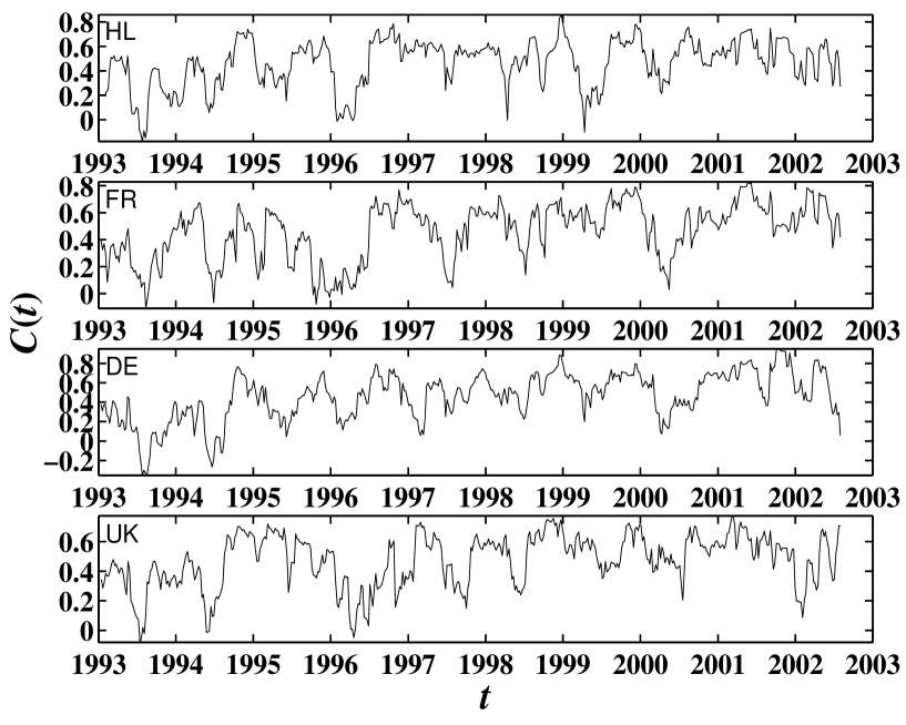
Figure 32: Cross-correlation coefficients between the USA S&P500 index and four European stock market indexes (Netherlands, France, Germany and United Kingdom from top to bottom) for weekly returns on filtered prices in a moving three-month window. Surrogate tests obtained by reshuffling the returns show that the large peaks and troughs are statistically significant. One can observe a slow overall increase of the correlation coefficient $C(t)$ over this decade. The variations are estimated to be $0.12$ by bootstrapping simulations.

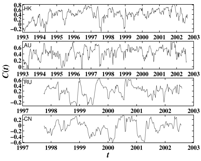
Figure 33: Cross-correlation coefficients between the USA S&P500 index and four non-European indexes (Hong Kong, Australia, Russia and China from top to bottom) for weekly returns on filtered prices in a moving three-month window. While one can observe a slow overall increase of the correlation coefficient $C(t)$ over this decade for Hong Kong and for Australia, no such trend is seen for Russia and China which are characterized by weaker correlations and more pronounced regime switches. The variations are estimated to be $0.12$ by bootstrapping simulations.

As illustrated in Fig. 32, the European markets have rather strong correlations with the American market with an average correlation coefficient of $0.44\pm 0.05$. The cross-correlation coefficients of the smoothed weekly returns for Hong Kong, Australia, Russia and China are shown in Fig. 33 as a function of time. Their average cross-correlation coefficients are relatively weaker than those for the European markets, with values respectively equal to $0.30\pm 0.05$, $0.34\pm 0.05$, $0.35\pm 0.05$ and $0.21\pm 0.05$ for Japan, Hong Kong, Australia and Russia. The average cross-correlation coefficient for China is slightly negative ($-0.06\pm 0.05$), indicating that the Chinese stock market seems practically uncorrelated from the western markets. The uncertainties and fluctuations of the variables $C(t)$ are determined by a bootstrap simulation of 1000 series of reshuffled returns which gives a standard deviation $\sigma_{C}=0.12$.

Interestingly, Fig. 32 shows that the cross-correlation coefficients of the European markets with the American market increases slowly with time. This property is weaker for Japan and Hong Kong and is completely absent for Russia and China. While qualitatively compatible, the evidence for a slow increase of the cross-correlation is not sufficiently precise to relate precisely to our previous finding of a strong synchronization of an anti-bubble regime since the summer of 2000.

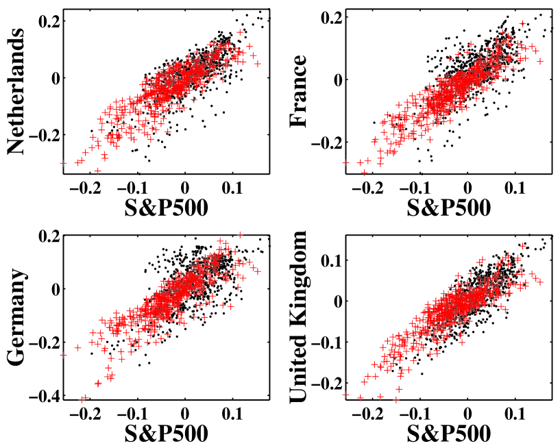
Figure 34: Monthly returns of four European market indices as a function of the monthly returns of the USA S&P500 index. The black dots correspond to period [Jun-04-1997, Aug-09-2000]. The $+$ correspond to the period [Aug-10-2000, Sep-04-2002].

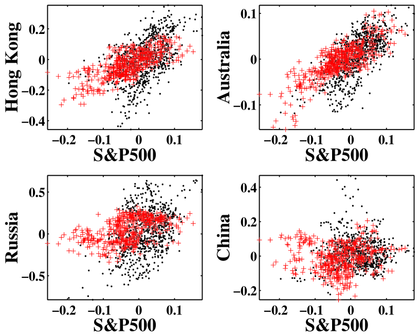
Figure 35: Weekly returns of four non-European market indices as a function of the weekly returns of the USA S&P500 index. The black dots correspond to period [Jun-04-1997, Aug-09-2000]. The $+$ correspond to the period [Aug-10-2000, Sep-04-2002].

To refine the evidence for an increase in correlation, we investigate the correlation between the USA S&P500 index and nine other indices (Netherlands (HL), France (FR), Japan (JP), Germany (DE), United Kingdom (UK), Hong Kong (HK), Australia (AU), Russia (RU), and China (CN)) in two periods, [Jun-04-1997, Aug-09-2000] and [Aug-10-2000, Sep-04-2002]. Table 8 shows the $\beta$ coefficients and corresponding correlation coefficients $\gamma$ of the weekly returns in these two periods. The coefficients $\beta_{1}$ and $\beta_{2}$ for the two periods of each index are obtained by using the well-known linear regression of the time series of returns of each index against the time series of returns of the S&P500 index. Such an approach led Roll [30] to conclude on the existence of a particularly strong synchronization during and after the crash of Oct. 1987 seen by the fact that the beta’s of the different indices against a world market index were anomalously large. The two correlation coefficients $\gamma_{1}$ and $\gamma_{2}$ are directly evaluated. The values of the slope $\beta$ [30] and the linear correlation coefficient $\gamma$ are listed in Table 8. Fig. 34 plots the returns of four European indices as a function of the returns of the S&P500 for each of the two periods. This figure and Table 8 confirm a significant increase of the correlations from the period [Jun-04-1997, Aug-09-2000] to the period [Aug-10-2000, Sep-04-2002]. Fig. 35 plots the returns of the indices of Hong Kong, Australia, Russia and China as a function of the returns of the S&P500 for each of the two periods. Table 8 and Fig. 35 show a significant increase in correlation from the period [Jun-04-1997, Aug-09-2000] to the period [Aug-10-2000, Sep-04-2002] only for Hong Kong and Australia. Russia gives a marginal signal and China none.

Table 8 and Fig. 34 clearly confirm a strong increase in the correlation between the USA stock market and the European indices and some non-European indices from the period [Jun-04-1997, Aug-09-2000] to the period [Aug-10-2000, Sep-04-2002], in agreement with the evidence of the log-periodic synchronization documented above.

3.2 Synchronization of weekly returns

We now discuss another intuitive measure for the characterization of the synchronization of weekly returns between different world stock markets. We use a moving window, whose size is 65 trading days, corresponding to 13 weeks. In this moving window, we define the synchronization factor $R(t)$ as the fraction of weeks among the 13 weeks for which a given index return has the same sign as that of the S&P500 index. By definition, $0\leq R(t)\leq 1$. $R(t)=1$ (respectively $R(t)=0$) corresponds to full synchronization (respectively perfect anti-synchronization). $R(t)=0.5$ corresponds to independent time series whose weekly returns have mutually random signs.

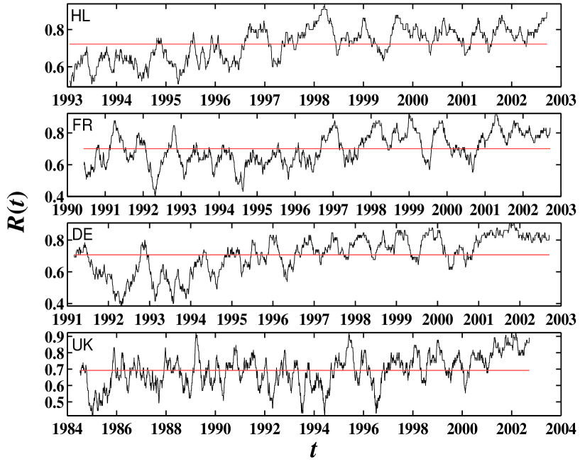
Figure 36: The synchronization factor $R(t)$ between the USA S&P500 index and four European indices (HL, FR, DE and UK), defined as the fraction of weeks with the same return signs over a moving 13-week window. The horizontal lines show the average of $R(t)$. The variations are estimated to be $0.06$ by bootstrapping simulations.

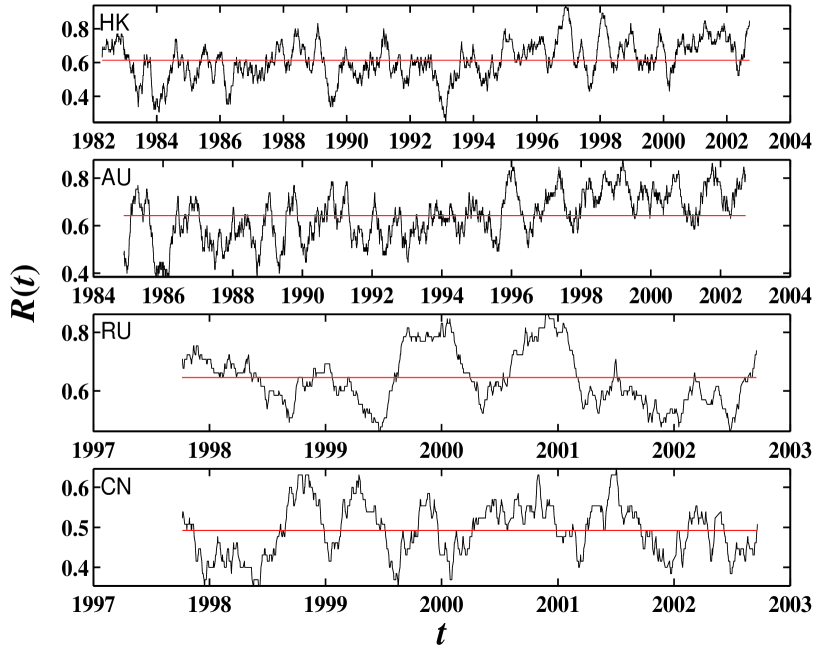
Figure 37: The synchronization factor $R(t)$ between the USA S&P500 index and four non-European indexes (HK, AU, RU and CN), defined as the fraction of weeks with the same return signs over a moving 13-week window. The horizontal lines show the average of $R(t)$. The variations are estimated to be $0.06$ by bootstrapping simulations.

We calculate the synchronization factor $R(t)$ between the USA S&P500 index and the indices of the Netherlands, France, Japan, Germany, UK, Hong Kong, Australia, Russia and China. As shown in Figs. 36 and 37, all considered indices have $R(t)$ significantly larger than $0.5$ except for China for which $R(t)=0.49$. The uncertainties and fluctuations of the variables $R(t)$ are determined by a bootstrap simulation of 1000 series of reshuffled returns which give a standard deviation $\sigma_{R}=0.06$. Again, the European markets have relatively higher synchronization factors and their $R(t)$ increase clearly with time. Not only $R(t)$ is consistently at its highest long-term average level in the last few years for all markets, except for Russia and China, we can also note a very strong and significant increase of $R(t)$ over the last year with much less fluctuations. Only Russia and China among the eight indices escape from this world-wide synchronization.

3.3 Time resolved event synchronization of the index time series

In view of the importance of characterizing the dependence between different markets, we present yet another measure of the synchronization of weekly returns across different world stock markets. The two previous analyses were based on the time series of weekly returns. The present analysis measures the synchronization between different index time series by quantifying the relative timings of specific events in the time series, following the algorithm initially introduced in [27].

Given two index time series $p^{(1)}(t)$ and $p^{(2)}(t)$, we define “events” as large market velocities. We define the market velocity as a coarse-grained measure of the slope of the price as a function of time. To obtain this coarse-grained measure, we apply on the prices $p(t)$ a causal Savitzky-Golay fourth-order polynomial filter with eight points on the left and no point on the right. The velocity $v(t)$ at time $t$ is define as the analytical time derivative of the coarse-grained $p(t)$. “Large velocities” are defined by the condition $|v(t)|>d$, where $d$ is a threshold chosen here equal to $d=0.001$. The times when the velocities $v^{(1)}(t)$ and $v^{(2)}(t)$ of the two index time series $p^{(1)}(t)$ and $p^{(2)}(t)$ obey the condition $|v(t)|>d$ are denoted respectively $t^{(1)}_{i}$ ($i=1,\ldots,m_{1}$) and $t^{(2)}_{j}$ ($j=1,\ldots,m_{2}$). The degree of synchronization is then quantified by counting the number of times an event ($|v(t)|>d$) appears in time series $p^{(1)}(t)$ shortly after it appears in time series $p^{(2)}(t)$. This number is estimated by the following formula

$$c(1|2)=\sum_{i=1}^{m_{1}}\sum_{j=1}^{m_{2}}J_{ij}$$ (10)

with

$$J_{ij}=\left\{\begin{array}[]{ll}1&{\mathtt{if~{}~{}}}0<t^{(1)}_{i}-t^{(2)}_{j}\leq\tau_{ij}\\ 1/2&{\mathtt{if~{}~{}}}t^{(1)}_{i}=t^{(2)}_{j}\\ 0&{\mathtt{otherwise}}\end{array}\right.,$$ (11)

where

$$\tau_{ij}=\min_{i,j}\left\{t^{(1)}_{i+1}-t^{(1)}_{i},~{}t^{(1)}_{i}-t^{(1)}_{i-1},~{}t^{(2)}_{j+1}-t^{(2)}_{j},~{}t^{(2)}_{j}-t^{(2)}_{j-1}\right\}~{}.$$ (12)

Likewise, $c(2|1)$ is calculated in a similar manner. The symmetrical combination

$$Q={{c(1|2)+c(2|1)}\over m_{1}m_{2}}~{},$$ (13)

called the synchronization index, measures the synchronization of the events and thus of the two time series. By construction, $0\leq Q\leq 1$. The cases of $Q=1$ and $Q=0$ correspond respectively to full synchronization and absence of synchronization of events of the two index time series.

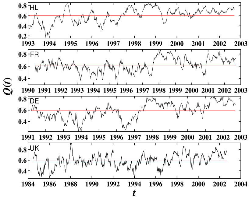
Figure 38: Synchronization index $Q(t)$ (see text and expression (13) for its definition) between the USA S&P500 index and four European stock indexes (HL, FR, DE and UK), as a function of time in a running window of 65 trading days. The horizontal lines show the average of $Q(t)$ over the shown time interval.

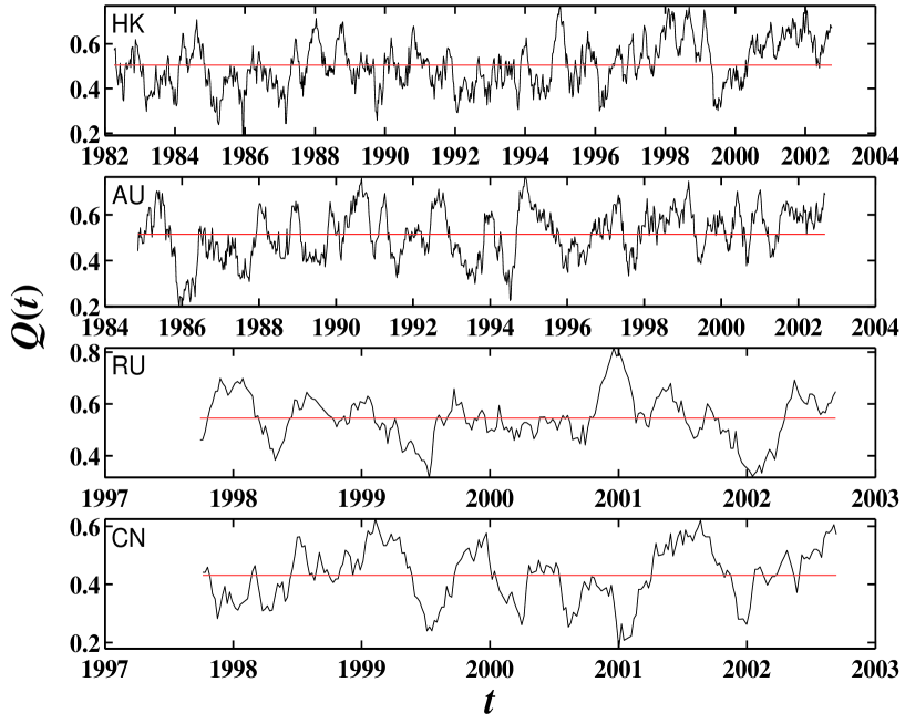
Figure 39: Same as Fig. 38 for four non-European indexes (HK, AU, RU and CN).

We calculate $Q(t)$ in a moving window of 65 trading days as before between the USA S&P500 index on the one hand and the stock markets of the Netherlands, France, Japan, Germany, UK, Hong Kong, Australia, Russia and China on the other hand. Fig. 38 and Fig. 39 shown that all stock markets have $Q(t)$ significantly larger than $0.5$ except for China. Again, an increasing trend appears clearly for the European markets. Furthermore, the period since the winter of 2000 has significantly larger $Q(t)$ compared with the earlier time for the European markets, Hong Kong and Australia. $Q(t)$ is especially large and regular for The Netherland (HL) since mid-1999 and all other markets also have a very high synchronization index $Q(t)$ since 2001.

4 Discussion

Following our previous investigation of the USA Standard and Poor index anti-bubble that started in August 2000 [43], we have analyzed the major stock market indices worldwide and found that a vast majority of European and Western countries as well as many other indices exhibit practically the same log-periodic power law anti-bubble structure as found for the USA S&P500 index. In addition, these anti-bubbles are found to start approximately at the same time, August 2000, in all these markets. This shows a remarkable degree of synchronization worldwide which, to our knowledge, has never been seen at any other time other than during and in the (short) aftermath of the October 1987 crash.

To test further this synchronization, we have also used several standard and less standard measures of correlation, dependence and synchronization between the USA S&P500 index and other world markets. These measures confirm the existence of significant increase of dependence in the last decade and still a larger increase in the last one-two years. However, these measures come nowhere close to the clarity of the signal of the extraordinary strong synchronization found using the log-periodic power law analysis. This is due to the fact that the log-periodic power law analysis is not sensitive to detailed phases in the oscillations (translated in slightly shifted effective time units in different markets) and detects only the robust universal unit-independent discrete scale invariant features of the price trajectories.

What triggered the worldwide anti-bubble in August 2000? The international descent of many of the worldwide stock markets since 2000 suggests the strengthening of globalization and the leading impact of the USA. In this respect, if history is any guide, the historical record on financial crises shows that they are often accompanying surges of globalization in the past, including events as far back as in the 19th century such as during the gold standard period of 1880-1913 [24]. Bordo and Murshid [4] compared various characteristics of the cross-country transmission of shocks in the financial markets of both advanced and emerging countries during two periods of globalization - the pre-World War I classical gold standard era, 1880-1914, and the post-Bretton Woods era, 1975-2000. They found that financial market shocks were more globalized before 1914 compared to the present and interpret this result by the growing financial maturity of advanced countries and the widening of the center to include a more diverse group of countries spanning several regions. Our findings temper Bordo and Murshid’s results and suggest a possible transition to a stronger integration and globalization fostered by several factors, including corporate and financial globalization, and the rapid development, adoption and use of information and communications technology. Our results also confirm those of Goetzmann et al. [9] who find that the correlation structure of the major world equity markets over 150 years vary considerably through time and are highest during periods of economic and financial integration such as the late 19th and 20th centuries. Goetzmann et al. [9] also stress that such increase of correlation implies that diversification benefits to global investing relies increasingly on investment in emerging markets, in agreement with our results on the weaker synchronization of emerging markets. Our results can also be seen to add to the literature on contagion, usually defined as correlation between markets in excess of what would be implied by economic fundamentals, by providing a new technical tool.

Acknowledgments: This work was supported in part by the James S. Mc Donnell Foundation 21st century scientist award/studying complex system.

Table 1: Parameters of the fits of the indices indicated in the first column using the first-order formula (1) from $t_{\rm{start}}$ to September, 30, 2002. All these indices are in the so-called bearish anti-bubble regime, qualified by the fact that the coefficient $B$ is negative. The exponents $\alpha$ of the leading power law in formula (1) are found either larger or smaller than $1$, corresponding to an accelerating (respectively decelerating) decrease of the prices as a function of time (see text). $\chi$ denotes the root-mean-square (r.m.s.).

Stock	$t_{\rm{start}}$	$t_{c}$	$\alpha$	$\omega$	$\phi$	$A$	$10^{3}B$	$10^{3}C$	$10^{2}\chi$
Netherlands	00/09/04	00/08/28	1.05	9.16	1.63	6.53	-0.55	-0.18	4.30
France	00/09/04	00/08/30	0.92	8.88	3.54	8.79	-1.39	-0.33	3.99
USA Dow Jones	00/09/06	00/08/15	1.05	9.76	4.01	9.30	-0.17	-0.11	3.37
USA NASDAQ	00/08/20	00/09/02	0.26	10.00	3.37	8.74	-251	-23.6	6.36
Japan	00/08/28	00/08/06	0.79	7.74	3.34	9.74	-3.40	-0.86	3.96
Belgium	00/11/06	00/06/25	1.52	12.20	2.85	8.02	-0.01	0.00	3.36
Denmark	00/10/24	00/05/03	0.78	13.37	0.62	5.98	-2.73	0.47	3.16
Germany	00/09/04	00/08/31	1.05	9.02	5.66	8.87	-0.57	0.19	4.39
Norway	00/09/05	00/10/02	1.02	8.21	4.77	6.75	-0.60	0.22	3.96
Spain	00/09/14	00/10/04	0.93	7.52	3.15	6.90	-0.82	0.31	3.98
Switzerland	00/08/23	00/11/18	1.00	6.76	5.16	9.01	-0.70	-0.26	3.67
UK	00/09/04	00/10/23	1.00	7.58	0.00	8.77	-0.55	-0.17	3.17
Israel	00/08/28	00/09/09	0.18	11.45	4.02	6.61	-205	17.7	4.51
Brazil	00/08/14	00/08/12	0.87	10.15	4.74	9.74	-1.36	0.56	6.20
Hong Kong	00/07/21	00/02/26	0.90	7.65	1.95	9.90	-1.69	-0.29	5.27
India	00/07/12	00/05/26	0.78	6.34	5.61	8.47	-2.92	-0.85	4.89
Peru	00/09/11	99/10/28	0.15	19.80	1.16	7.45	-118	-20.9	3.22
Taiwan	00/07/17	00/01/24	0.38	9.22	1.01	9.26	-63.0	17.7	8.50
Czech	00/07/28	00/08/13	0.53	4.61	1.19	6.32	-12.5	5.20	4.80
Argentina	00/07/14	00/05/02	1.54	7.25	5.28	6.23	-0.03	-0.02	12.2
Turkey	00/07/10	00/08/28	0.13	9.56	2.88	9.62	-160	63.7	11.8

Table 2: Values of the parameters of the fits to the 21 indices of table 1 given in the first column using formula (4) from $t_{\rm{start}}$ to September, 30, 2002. As in table 1, the bearish nature of the markets is identified by the fact that $B<0$. Note that the amplitude $D$ of the harmonics is often very significant compared with the amplitude $C$ of the mean angular log-frequency.

Stock	$t_{\rm{start}}$	$t_{c}$	$\alpha$	$\omega$	$\phi_{1}$	$\phi_{2}$	$A$	$10^{3}B$	$10^{3}C$	$10^{3}D$	$10^{2}\chi$
Netherlands	00/09/04	00/07/20	0.80	11.07	4.75	0.91	6.60	-2.82	0.64	0.32	3.72
France	00/09/04	00/07/04	0.71	11.24	0.28	4.25	8.90	-5.76	-0.91	0.48	3.47
USA DowJones	00/09/06	00/06/18	0.72	12.09	0.83	2.16	9.33	-1.45	-0.65	-0.34	3.00
USA NASDAQ	00/08/20	00/09/02	0.26	10.00	3.37	0.00	8.77	-269.2	-24.73	-9.18	5.70
Japan	00/08/28	00/08/06	0.77	7.74	3.35	0.00	9.74	-3.72	-0.89	0.21	3.69
Belgium	00/11/06	00/06/21	1.14	12.24	2.67	0.49	8.05	-0.12	0.05	-0.02	2.83
Denmark	00/10/24	00/05/04	0.64	13.35	0.87	0.00	6.04	-7.51	1.05	0.36	2.86
Germany	00/09/04	00/10/06	0.94	8.47	3.61	4.58	8.86	-1.20	0.41	0.12	3.96
Norway	00/09/05	00/07/13	0.87	10.92	2.03	1.78	6.82	-1.61	-0.45	0.13	3.58
Spain	00/09/14	99/07/03	0.88	15.70	1.75	1.28	7.14	-1.14	-0.18	0.08	3.46
Switzerland	00/08/23	00/11/23	0.95	6.72	5.54	0.00	9.01	-0.98	-0.35	-0. 07	3.52
UK	00/09/04	00/07/21	0.84	10.78	3.56	1.52	8.83	-1.53	-0.30	-0.16	2.82
Israel	00/08/28	00/09/09	0.19	11.41	4.26	0.00	6.60	-194.	17.28	-1.73	4.49
Brazil	00/08/14	00/02/23	1.08	7.99	6.24	4.69	9.83	-0.34	-0.07	-0.08	5.41
HongKong	00/07/21	00/01/30	0.41	7.52	2.21	0.41	10.39	-71.68	-4.88	3.03	4.63
India	00/07/12	99/12/04	0.03	8.84	5.96	0.73	17.34	-7544	-63	39.5	4.12
Peru	00/09/11	00/02/26	0.54	7.69	2.98	4.99	7.19	-1.67	1.20	1.92	2.76
Taiwan	00/07/17	99/05/07	0.31	7.34	1.93	4.44	9.95	-181.0	-14.51	21.50	5.41
Czech	00/07/28	00/08/11	0.40	4.59	1.27	0.77	6.39	-33.90	9.69	-4.46	3.94
Argentina	00/07/14	99/08/23	2.00	11.23	0.67	4.40	6.25	-0.00	-0.00	0.00	8.20
Turkey	00/07/10	00/08/28	0.20	9.55	2.94	1.32	9.52	-78.16	47.12	18.47	11.0

Table 3: Values of the parameters of the fits of the indices indicated in the first column using the first-order formula (1) from $t_{\rm{start}}$ to September, 30, 2002. The bullish nature of the markets refers to the the fact that $B>0$. The exponents $\alpha$ of the leading power law take values either greater or less than 1 indicating either an upward or a downward overall large scale curvature of the price trajectory.

Stock	$t_{\rm{start}}$	$t_{c}$	$\alpha$	$\omega$	$\phi$	$A$	$10^{3}B$	$10^{3}C$	$10^{2}\chi$
Australia	00/09/04	00/08/08	0.77	10.85	3.55	8.08	0.07	-0.37	1.76
Mexico	00/09/04	00/08/08	0.80	10.11	4.42	8.70	0.32	0.86	4.02
Indonesia	00/09/16	00/08/09	1.06	10.30	5.83	5.99	0.09	-0.21	3.90
Korea	00/10/12	00/11/15	1.37	6.69	5.67	6.29	0.05	-0.05	5.00
Thailand	00/09/20	00/08/16	0.93	9.45	5.16	5.61	0.58	-0.39	4.37
Russia	00/12/01	00/10/08	0.92	7.93	3.33	7.24	2.76	-0.68	4.85

Table 4: Values of the parameters of the fits of the indices indicated in the first column using formula (4) from $t_{\rm{start}}$ to September, 30, 2002.

Stock	$t_{\rm{start}}$	$t_{c}$	$\alpha$	$\omega$	$\phi_{1}$	$\phi_{2}$	$A$	$10^{3}B$	$10^{3}C$	$10^{3}D$	$10^{2}\chi$
Australia	00/09/04	00/08/10	0.64	10.89	3.42	0.51	8.08	0.26	-0.80	-0.26	1.53
Mexico	00/09/04	00/06/27	0.73	5.97	4.23	1.65	8.69	0.72	0.39	-1.15	3.91
Indonesia	00/09/16	00/11/16	0.96	3.47	1.33	3.10	6.04	-0.25	-0.50	-0.62	2.71
Korea	00/10/12	00/08/10	1.00	5.04	1.90	1.90	6.24	0.46	-0.23	-0.25	4.28
Thailand	00/09/20	00/07/27	0.43	5.18	3.62	2.22	5.48	20.83	3.90	6.62	3.54
Russia	00/12/01	00/10/12	0.91	7.85	3.90	0.17	7.23	3.07	-0.75	0.10	4.57

Table 5: Likelihood-ratio (Wilk) test of hypothesis $H_{1}$ against $H_{0}$ and of hypothesis $H_{2}$ against $H_{1}$, where $H_{0}$ is the hypothesis that $C=0$ in (1) (pure power law fit), $H_{1}$ is the hypothesis that $D=0$ in (4) (corresponding to the log-periodic function (1) without any harmonics) and $H_{2}$ is the hypothesis that $D\neq 0$, corresponding to the log-periodic function (4) which includes an harmonic at $2\omega$. Each stock index time series whose country/area is given in the first column starts at $t_{\rm{start}}$ and ends at September 30, 2002. The column $n$ gives the number of the data points for each fit. The $\sigma_{j}$’s are the standard deviations for hypothesis $H_{j}$ with $j=0,1,2$ of the fits to the data associated with formula (1) and (4). The $T_{j,j+1}$ are the log-likelihood-ratios defined in expression (8). The $P_{j,j+1}$ are the probability for exceeding $T_{j,j+1}$ under the assumption of that hypothesis $H_{j}$ holds.

Stock	$t_{\rm{start}}$	$n$	$\sigma_{0}$	$\sigma_{1}$	$\sigma_{2}$	$T_{0,1}$	$T_{1,2}$	${\rm{P}}_{0,1}(\%)$	${\rm{P}}_{1,2}(\%)$
Netherlands	00/09/04	508	0.078	0.043	0.037	609.2	148.5	$<10^{-4}$	$<10^{-4}$
France	00/09/04	520	0.070	0.040	0.035	589.0	144.2	$<10^{-4}$	$<10^{-4}$
USA DowJones	00/09/06	500	0.053	0.034	0.030	459.8	118.1	$<10^{-4}$	$<10^{-4}$
USA NASDAQ	00/08/20	511	0.099	0.064	0.057	456.2	111.5	$<10^{-4}$	$<10^{-4}$
Japan	00/08/28	498	0.069	0.040	0.037	551.7	70.7	$<10^{-4}$	$<10^{-4}$
Belgium	00/11/06	459	0.056	0.034	0.028	466.7	158.6	$<10^{-4}$	$<10^{-4}$
Denmark	00/10/24	456	0.052	0.032	0.029	457.1	92.2	$<10^{-4}$	$<10^{-4}$
Germany	00/09/04	504	0.083	0.044	0.040	637.9	105.7	$<10^{-4}$	$<10^{-4}$
Norway	00/09/05	543	0.081	0.040	0.036	772.0	110.8	$<10^{-4}$	$<10^{-4}$
Spain	00/09/14	483	0.062	0.040	0.035	421.9	133.0	$<10^{-4}$	$<10^{-4}$
Switzerland	00/08/23	505	0.062	0.037	0.035	526.9	40.9	$<10^{-4}$	$<10^{-4}$
UK	00/09/04	506	0.050	0.032	0.028	464.5	120.4	$<10^{-4}$	$<10^{-4}$
Israel	00/08/28	390	0.058	0.045	0.045	194.0	2.7	$<10^{-4}$	$10.03$
Brazil	00/08/14	505	0.094	0.062	0.054	418.9	138.0	$<10^{-4}$	$<10^{-4}$
HongKong	00/07/21	523	0.070	0.053	0.046	298.3	135.6	$<10^{-4}$	$<10^{-4}$
India	00/07/12	528	0.073	0.049	0.041	428.7	180.2	$<10^{-4}$	$<10^{-4}$
Peru	00/09/11	488	0.051	0.032	0.028	438.3	151.9	$<10^{-4}$	$<10^{-4}$
Taiwan	00/07/17	518	0.114	0.085	0.054	307.3	466.7	$<10^{-4}$	$<10^{-4}$
Czech	00/07/28	507	0.052	0.048	0.039	72.4	199.0	$<10^{-4}$	$<10^{-4}$
Argentina	00/07/14	502	0.148	0.122	0.082	194.0	401.1	$<10^{-4}$	$<10^{-4}$
Turkey	00/07/10	534	0.146	0.118	0.110	233.1	67.8	$<10^{-4}$	$<10^{-4}$
Australia	00/09/04	509	0.031	0.018	0.015	588.4	144.1	$<10^{-4}$	$<10^{-4}$
Mexico	00/09/04	493	0.078	0.040	0.039	655.4	25.9	$<10^{-4}$	$\approx 10^{-4}$
Indonesia	00/09/16	454	0.080	0.039	0.027	658.6	329.1	$<10^{-4}$	$<10^{-4}$
Korea	00/10/12	456	0.108	0.050	0.043	705.2	142.3	$<10^{-4}$	$<10^{-4}$
Thailand	00/09/20	481	0.076	0.044	0.035	535.1	203.0	$<10^{-4}$	$<10^{-4}$
Russia	00/12/01	413	0.114	0.048	0.046	704.7	48.1	$<10^{-4}$	$<10^{-4}$

Table 6: Fitting parameters with equation (1) for the French market stock index with different $t_{\rm{start}}$ indicated in the first column.

$t_{\rm{start}}$	$t_{c}$	$\alpha$	$\omega$	$\phi$	$A$	$B$	$C$	$\chi$
00/06/01	00/08/20	0.91	9.23	4.26	8.81	-0.00154	0.00035	0.0387
00/07/01	00/08/15	0.89	9.53	5.48	8.81	-0.00168	-0.00038	0.0389
00/08/01	00/08/19	0.89	9.36	3.45	8.81	-0.00165	0.00038	0.0393
00/09/01	00/08/30	0.91	8.90	3.37	8.79	-0.00145	-0.00035	0.0399
00/10/01	00/10/23	0.97	7.56	3.19	8.74	-0.00101	0.00029	0.0400
00/11/01	00/10/25	0.98	7.46	0.70	8.74	-0.00096	-0.00027	0.0407
00/12/01	00/10/23	1.05	7.48	0.50	8.72	-0.00061	-0.00018	0.0413

Table 7: Fitting parameters with equation (1) for the Australian market stock index with different $t_{\rm{start}}$ indicated in the first column.

$t_{\rm{start}}$	$t_{c}$	$\alpha$	$\omega$	$\phi$	$A$	$B$	$C$	$\chi$
00/06/01	00/09/23	0.76	9.41	0.88	8.08	0.00002	-0.00044	0.0173
00/07/01	00/08/21	0.80	10.25	4.42	8.09	0.00001	0.00032	0.0173
00/08/01	00/08/20	0.78	10.29	4.17	8.09	0.00002	0.00036	0.0176
00/09/01	00/08/14	0.77	10.57	2.29	8.08	0.00006	0.00037	0.0176
00/10/01	00/08/11	0.78	10.68	4.67	8.08	0.00007	-0.00035	0.0177
00/11/01	00/09/26	0.72	9.35	4.47	8.08	0.00003	0.00055	0.0180
00/12/01	00/09/11	0.67	9.78	4.66	8.08	0.00007	-0.00073	0.0181

Table 8: $\beta$’s and correlation coefficients $\gamma$ between the USA S&P500 index and nine indices (Netherlands (HL), France (FR), Japan (JP), Germany (DE), United Kingdom (UK), Hong Kong (HK), Australia (AU), Russia (RU), and China (CN)) in two periods. Period $1$ is [Jun-04-1997, Aug-09-2000] and period $2$ is [Aug-10-2000, Sep-04-2002]. The return is the logarithm of the ratio between two successive prices with time lag of 30 trading days.

INDEX	HL	FR	JP	DE	UK	HK	AU	RU	CN
$\beta_{1}$	1.07	0.93	0.98	0.92	0.68	1.34	0.60	2.21	-0.05
$\gamma_{1}$	0.73	0.67	0.62	0.83	0.49	0.51	0.68	0.42	0.03
$\beta_{2}$	1.06	1.03	1.17	0.76	0.66	0.92	0.45	0.99	0.02
$\gamma_{2}$	0.87	0.90	0.86	0.87	0.59	0.72	0.80	0.46	0.02

Figure 9: The stock market index of Norway (fine line) and its fits with the simple log-periodic formula (1) (thick line) and with formula (4) incorporating an harmonics (dashed line). The starting date for the fits is $t_{\rm{start}}=$ 05-Sep-2000. The parameter values of the fit with (1) are $t_{c}=$ 02-Oct-2000, $\alpha=1.02$, $\omega=8.21$, $\phi=4.77$, $A=6.75$, $B=-0.00060$, and $C=0.00022$. The r.m.s. of the fit errors is 0.0396. The parameter values of the fit with (4) are $t_{c}=$ 13-Jul-2000, $\alpha=0.87$, $\omega=10.92$, $\phi_{1}=2.03$, $\phi_{2}=1.78$, $A=6.82$, $B=-0.00161$, $C=-0.00045$, and $D=0.00013$. The r.m.s. of the fit errors is 0.0358. The formula including the harmonics reduces the r.m.s. of fit errors by 9.7%.

References

- [1] Barro R.J., E.F. Fama, D.R. Fischel, A.H Meltzer, R. Roll and L.G. Telser, Black monday and the future of financial markets, in: R.W. Kamphuis, Jr., R.C. Kormendi and J.W.H. Watson, eds., Mid American Institute for Public Policy Research, Inc. and Dow Jones-Irwin, Inc. (1989).
- [2] Blanchard, O.J., Speculative Bubbles, Crashes and Rational Expectations, Economics Letters 3, 387-389 (1979).
- [3] Blanchard, O.J. and M.W. Watson, Bubbles, Rational Expectations and Speculative Markets, in: Wachtel, P. ,eds., Crisis in Economic and Financial Structure: Bubbles, Bursts, and Shocks. Lexington Books: Lexington (1982).
- [4] Bordo, M.D. and A.P. Murshid, Globalization and Changing Patterns in the International Transmission of Shocks in Financial Markets, NBER Working Paper No. W9019 (2002)
- [5] Cass, D., Sunspots and incomplete financial markets: The General case, Philadelphia, University of Pennsylvania (1991).
- [6] Cvijovic, D. and J. Klinowski, Taboo Search: An Approach to the Multiple Minima Problem, Science 267, 664-666 (1995).
- [7] Drozdz, S., Ruf, F., Speth, J. and Wojcik, M., Imprints of log-periodic self-similarity in the stock market, European Physical Journal 10, 589-593 (1999).
- [8] Gluzman, S. and D. Sornette, Log-periodic route to fractal functions, Phys. Rev. E 65, 036142 (2002).
- [9] Goetzmann, W.N., L. Li and K.G. Rouwenhorst, Long-Term Global Market Correlations, NBER Working Paper No. W8612 (2001)//
- [10] Holden K, Peel D.A. and Thompson J.L., Economic Forecasting: An Introduction (Cambridge University Press, Cambridge, 1990) pp.59.
- [11] Ide, K. and D. Sornette, Oscillatory Finite-Time Singularities in Finance, Population and Rupture, Physica A 307 (1-2), 63-106 (2002).
- [12] Johansen, A., Comment on “Are financial crashes predictable?” Europhys. Lett. 60, 809-810 (2002). see also Remarks on reply to Johansen’s comment, at cond-mat/0206479
- [13] Johansen, A., O. Ledoit and D. Sornette, Crashes as critical points, International Journal of Theoretical and Applied Finance 3, 219-255 (2000).
- [14] Johansen, A. and D. Sornette, Stock market crashes are outliers, European Physical Journal B 1, 141-143 (1998).
- [15] Johansen, A. and D. Sornette, Financial “anti-bubbles”: Log-periodicity in Gold and Nikkei collapses, Int. J. Mod. Phys. C 10, 563-575 (1999).
- [16] Johansen, A. and D. Sornette, Critical Crashes, RISK 12, 91-94 (1999).
- [17] Johansen, A. and D. Sornette, Bubbles and anti-bubbles in Latin-American, Asian and Western Stock markets: An emprical study, Int. J. Theor. Appl. Fin. 4, 853-920 (2000).
- [18] Johansen, A. and D. Sornette, Evaluation of the quantitative prediction of a trend reversal on the Japanese stock market in 1999, Int. J. Mod. Phys. C 11, 359-364 (2000).
- [19] Johansen, A. and D. Sornette, The Nasdaq crash of April 2000: Yet another example of log-periodicity in a speculative bubble ending in a crash, Eur. Phys J. B 17, 319-328 (2000).
- [20] Johansen, A. and D. Sornette, Large Stock Market Price Drawdowns Are Outliers, Journal of Risk 4, 69-110 (2002).
- [21] Johansen, A. and D. Sornette, Endogenous versus Exogenous Crashes in Financial Markets, preprint at cond-mat/0210509.
- [22] Johansen, A., D. Sornette and O. Ledoit, Predicting financial crashes using discrete scale invariance, Journal of Risk 1, 5-32 (1999).
- [23] Lux, T. and D. Sornette, On Rational Bubbles and Fat Tails, Journal of Money, Credit and Banking part 1, vol. 34, No. 3, 589-610 (2002).
- [24] Neal, L.D. and M. Weidenmier, Crises in the Global Economy from Tulips to Today: Contagion and Consequences, NBER Working Paper No. W9147 (2002) preprint at
- [25] Malevergne, Y. and D. Sornette, Multi-dimensional Rational Bubbles and fat tails, Quantitative Finance 1, 533-541 (2001).
- [26] Press, W., S. Teukolsky, W. Vetterling and B. Flannery, Numerical Recipes in FORTRAN: The Art of Scientific Computing (Cambridge University, Cambridge, 1996).
- [27] Quiroga, R., T. Kreuz and P. Grassberger, Event synchronization: a simple and fast method to measure synchronicity and time delay patterns, Phys. Rev. E 66, 041904 (2002).
- [28] Rao, C., Linear statistical Inference and Its Applications (New York, Wiley, 1965) chap. 6, section 6e.3.
- [29] Roehner, B.M. and D. Sornette, “Thermometers” of Speculative Frenzy, European Physical Journal B 16, 729-739 (2000).
- [30] Roll, R., The International Crash of October 1987, in Black Monday and The Future of Financial Markets, edited by A. Meltzer, Dow-Jones-Irwin (1988).
- [31] Shefrin, H., Beyond greed and fear: understanding behavioral finance and the psychology of investing (Boston, Mass.: Harvard Business School Press, 2000).
- [32] Shiller, R.J., Market volatility (Cambridge, Mass.: MIT Press, 1989).
- [33] Shiller, R.J., Irrational exuberance (Princeton University Press, Princeton, NJ., 2000).
- [34] Shleifer, A., Inefficient markets: an introduction to behavioral finance (New York: Oxford University Press, 2000).
- [35] Sornette, D., Discrete scale invariance and complex dimensions, Physics Reports 297, 239-270 (1998).
- [36] Sornette, D., Why Stock Markets Crash (Critical Events in Complex Financial Systems), Princeton University Press, Princeton, NJ, 2003.
- [37] Sornette, D. and J.V. Andersen, A Nonlinear Super-Exponential Rational Model of Speculative Financial Bubbles, Int. J. Mod. Phys. C 13, 171-188 (2002).
- [38] Sornette, D. and K. Ide, Theory of self-similar oscillatory finite-time singularities in Finance, Population and Rupture, Int. J. Mod. Phys. C 14, 267-275 (2002).
- [39] Sornette, D. and A. Johansen, A Hierarchical Model of Financial Crashes, Physica A 261, 581-598 (1998).
- [40] Sornette, D. and A. Johansen, Significance of log-periodic precursors to financial crashes, Quantitative Finance 1, 452-471 (2001).
- [41] Sornette, D., A. Johansen and J.-P. Bouchaud, Stock market crashes, Precursors and Replicas, J.Phys.I France 6, 167-175 (1996).
- [42] Sornette, D. and Y. Malevergne, From Rational Bubbles to Crashes, Physica A 299, 40-59 (2001).
- [43] D. Sornette and W.-X. Zhou, The US 2000-2002 Market Descent: How Much Longer and Deeper? Quantitative Finance 2, 468-481 (2002).
- [44] Zhou, W.-X. and Didier Sornette, Statistical Significance of Periodicity and Log-Periodicity with Heavy-Tailed Correlated Noise, Int. J. Mod. Phys. C 13, 137-170 (2002).