New Collective Modes in the Superconducting Ground States in the Gauge Theory Description of the Cuprates

Abstract

In the slave boson mean field treatment of the $t$-$J$ model, the ground state for small doping is a $d$-wave superconductor. A conventional superconductor has collective modes associated with the amplitude and phase of the pairing order parameter. Here, the hopping matrix element $\chi_{ij}$ is also a mean field order parameter. We therefore expect that new collective modes will be introduced with these additional complex degrees of freedom. We compute the new collective modes and their spectral functions by numerically diagonalizing the matrix which describes the fluctuations about the mean field solution. We also show that the SU(2) gauge theory formulation allows us to predict and classify these collective modes. Indeed, the SU(2) formulation is essential in order to avoid spurious collective modes as the doping $x$ goes to zero. The most important new collective modes are the $\theta$ mode and the longitudinal and transverse $\phi$ gauge modes. The $\theta$ mode corresponds to fluctuations of the staggered flux phase and creates orbital current fluctuations. The $\phi$ gauge modes correspond to out-of-phase fluctuations of the amplitudes of the pairing and the hopping matrix elements. We compute the neutron scattering cross-section which couples to the $\theta$ mode and inelastic X-ray scattering cross-section which couples to the fluctuation in the real part of $\chi_{ij}$. In addition, we show that the latter fluctuation at $(\pi,\pi)$ may be coupled to the buckling phonon mode in the LTO phase of LSCO and may be detected optically. Experimental searches of these collective modes will serve as important tests of this line of attack on the high T_c problem.

I Introduction

It is now a widely accepted view that the problem of high T_c superconductivity is that of doping into a Mott insulator. The simplest model which captures the physics of the strong correlation inherent in this problem is the $t$-$J$ model. The no-double-occupant constraint leads naturally to a gauge theory. The mean field decoupling of this theory is the formal language which describes Anderson’s physical idea of a resonating valence bond (RVB).[1] The mean field theory indeed enjoys a number of successes. Notably it predicted the appearance of $d$-wave superconductivity and the existence of a spin gap phase in the underdoped region.[2, 3, 4] The properties of this spin gap phase are in remarkable agreement with those of the pseudogap phenomenology. Most striking among these is that the quasiparticle spectral function becomes a coherent peak with small spectral weight. This property emerges naturally out of the mean field picture of the condensation of bosons.

Despite these successes, the theory has not enjoyed wide following because the gauge fluctuations are strong and the theory does not have a well controlled small expansion parameter, except formal ones such as the large $N$ expansion. For example, Nayak[5] has raised a number of objections on general grounds. However, we believe these general arguments have been adequately answered in the ensuing comments and discussions.[6, 7, 8, 9] Here we briefly summarize our point of view.

Initially, the gauge field has infinite coupling in order to enforce the constraint on a lattice scale. Upon integrating out high energy fermionic degrees of freedom, the coupling constant becomes of order unity. Then there is a chance that the mean field theory and fluctuations about it may be qualitatively correct at intermediate temperature scales. At low energy scales, nonperturbative effects related to compact gauge theories may come in, giving rise to the phenomenon of confinement. This phenomenon is well known at half-filling. The mean field solution gives a $\pi$-flux state with Dirac spectrum centered about $\left(\pm{\pi\over 2},\pm{\pi\over 2}\right)$. Coupling with compact U(1) gauge field leads to confinement and chiral symmetry breaking in particle physics language, which is equivalent to Néel ordering.[10] The idea is that with doping, the appearance of dissipation suppresses confinement,[11] and the Néel state is rapidly destroyed. Then the mean field description may be qualitatively correct beyond a small, but finite, doping concentration. At low temperatures characterized by the boson condensation scale $xt$, superconductivity emerges. In this theory the superconducting state is described as the Higgs phase associated with bose condensation. (We prefer to refer to this as the Higgs phase rather than bose condensation because the bose field is not gauge invariant.) However, here lies one of the significant failures of the weak coupling gauge theory description. As long as the gauge fluctuation is treated as Gaussian, the Ioffe-Larkin law holds and one predicts that the superfluid density $\rho_{s}(T)$ behaves as $\rho_{s}(T)\approx ax-bx^{2}T$. The $ax$ term agrees with experiment while the $-bx^{2}T$ term does not.[12, 13] This failure is traced to the fact that in the Gaussian approximation, the current carried by the quasiparticles in the superconducting state is proportional to $xv_{F}$. We believe this failure is a sign that nonperturbative effects again become important and confinement takes place, so that the low energy quasiparticles near the nodes behave like BCS quasiparticles which carry the full current $v_{F}$. For the pure gauge theory, the confinement always occurs in (2+1)D however small the coupling constant of the gauge field is. When the bose field is coupled to the gauge field, i.e., Higgs model, it is known that the confinement phase are smoothly connected to each other.[14] Recently, we showed that in (2+1)D Higgs model the phase should be considered confined everywhere.[15] Thus the appearance of confinement at low energy scale is not surprising, but the dichotomy between the success of the bose condensation phenomenology on the one hand (in explaining the quasiparticle spectral weight mentioned earlier) and the confinement physics needed to give the proper quasiparticle currents on the other, is in our opinion one of the most profound questions facing the field today.

To summarize, the current status of the gauge theory approach to the $t$-$J$ model is the following. Within mean field theory, a certain saddle-point solution may be regarded as the “mother state” at some intermediate energy scale. The most promising candidate for this “mother state” appears to be the staggered flux state, which is the saddle point for the SU(2) formulation of the $t$-$J$ model. This saddle point is an unstable fixed point due to gauge fluctuations. It flows to the Néel state at or near half filling and to the superconducting ground state at finite doping. This picture is in accordance with a recent insightful comment by Anderson,[16] except that we provide a concrete description of the unstable fixed point. As discussed above, the issues raised by this picture are profound and probably difficult to treat analytically. In the past few years, we have focused on trying to substantiate this point of view by numerical methods and by predicting new experiments. On the numerical front, the study of projected wavefunctions have yielded remarkable insights. Ivanov et al.[17] reported a finding which is surprising except from the SU(2) gauge theory point of view. They discovered that upon Gutzwiller projection of a BCS $d$-wave state, the current-current correlation shows a staggered pattern, as expected for the staggered flux state. Thus there is strong numerical evidence that the staggered flux state and the $d$-wave superconducting state are intimately related. On the experimental front, predictions have been made that the staggered flux state may be stabilized in the vortex core and ways to measure the effect of the orbital currents have been proposed.[18] In this paper we continue work in this direction and ask the question: is the superconducting ground state that emerges out of the gauge theory completely conventional, or are there detectable consequences of its unconventional origin?

The short answer to this question is that gauge theory predicts new collective modes in the superconducting ground state which have experimental consequences. Unlike conventional BCS theory, where the only order parameter is the complex pairing order parameter $\Delta$, here the hopping matrix element $\chi$ also functions as an order parameter. Thus it is natural to expect new collective modes. This problem is formulated generally in Sections II and III. In Section IV we show how the gauge theory allows us to predict the low lying collective modes. The new modes are the $\theta$ mode and the transverse and longitudinal $\phi$ modes. The $\theta$ mode generates staggered orbital current fluctuations and is related to the current fluctuations found in the projected wavefunctions. However, while the projected wavefunctions give only equal time correlation, here we obtain the full dynamical spectral function. The $\phi$ gauge modes are new excitations related to amplitude fluctuations of $\chi$ and $\Delta$. In Sections V and VI we present numerical results of the spectral functions and describe experiments which may couple to them.

The approximation employed in this paper is to treat the system in the Higgs phase by adopting the radial gauge for the bosons. Gauge fluctuations are treated at the Gaussian level and nonanalytic corrections, such as instantons which may lead to confinement, are neglected. This can be justfied in terms of the $1/N$-expansion with $N$ being the number of fermion species. In the present case, $N=2$ and one criterion for the validity of this Gaussian approximation is that the magnitude of the order parameter fluctuation is less than that of the mean field value. As is evident from the discussion in II and III, the magnitude of the fluctuation diverges as $x\to 0$ because the action for the SU(2) local gauge transformation vanishes in this limit. Hence the Gaussian approximation breaks down near $x=0$, where the confinement physics is of vital importance because the nonperturbative configurations such as instantons contribute appreciably. Below we will show mainly the numerical results for $x=0.1$. We have estimted numerically the magnitude of the fluctuation of the order parameters, e.g., $<(\delta\chi_{x})^{2}>$ at zero temperature, and found that it is of the order of unity at $x=0.1$. Therefore the gaussian approximation is marginaly justified in this case. As another test, recently Honerkamp and Lee [19] have computed the shift in $\Delta$ using a free energy which includes the gaussian fluctuaions of the $\theta$ mode. They found a reduction to 55 $\%$ of the mean field saddle point value for x=.06 but for x=.1 the reduction is only 80 $\%$. Thus the effect of the gaussian fluctuation is relatively under control for increasing doping. Furthermore, since the collective modes appear at fairly high energy $(\sim J)$ for experimentally relevant doping $(x\approx 0.1)$, it is possible that this approximation is valid at this energy scale, but the ultimate test must come from experiment.

II U(1) and SU(2) Formulations of the $t$-$J$ Model

We begin with the familiar U(1) formulation of the $t$-$J$ model[20]

$$H=\sum_{<i,j>}J\left({\mathchoice{{\hbox{\boldmath$\displaystyle S$}}}{{\hbox{\boldmath$\textstyle S$}}}{{\hbox{\boldmath$\scriptstyle S$}}}{{\hbox{\boldmath$\scriptscriptstyle S$}}}}_{i}\cdot{\mathchoice{{\hbox{\boldmath$\displaystyle S$}}}{{\hbox{\boldmath$\textstyle S$}}}{{\hbox{\boldmath$\scriptstyle S$}}}{{\hbox{\boldmath$\scriptscriptstyle S$}}}}_{j}-{1\over 4}n_{i}n_{j}\right)-t_{ij}c_{i\sigma}^{\dagger}c_{j\sigma}.$$ (1)

The constraint of no double occupation is enforced by writing

$$c_{i\sigma}^{\dagger}=f_{i\sigma}^{\dagger}b_{i}$$ (2)

and imposing the condition $\sum_{\sigma}f_{i\sigma}^{\dagger}f_{i\sigma}+b^{\dagger}_{i}b_{i}=1$, which in turn is enforced with a Lagrangian multiplier $\lambda_{i}$. The Heisenberg exchange term is written in terms of $f_{i\sigma}$[21]

$${\mathchoice{{\hbox{\boldmath$\displaystyle S$}}}{{\hbox{\boldmath$\textstyle S$}}}{{\hbox{\boldmath$\scriptstyle S$}}}{{\hbox{\boldmath$\scriptscriptstyle S$}}}}_{i}\cdot{\mathchoice{{\hbox{\boldmath$\displaystyle S$}}}{{\hbox{\boldmath$\textstyle S$}}}{{\hbox{\boldmath$\scriptstyle S$}}}{{\hbox{\boldmath$\scriptscriptstyle S$}}}}_{j} = -{1\over 4}f_{i\sigma}^{\dagger}f_{j\sigma}f_{j\beta}^{\dagger}f_{i\beta}$$ (3)

$$- {1\over 4}\left(f_{i\uparrow}^{\dagger}f_{j\downarrow}^{\dagger}-f_{i\downarrow}^{\dagger}f_{j\uparrow}^{\dagger}\right)\left(f_{j\downarrow}f_{i\uparrow}-f_{j\uparrow}f_{i\downarrow}\right)$$ (4)

$$+ {1\over 4}\left(f_{i\alpha}^{\dagger}f_{i\alpha}\right).$$ (5)

We write

$$n_{i}n_{j}=(1-b_{i}^{\dagger}b_{i})(1-b_{j}^{\dagger}b_{j}).$$ (6)

Then ${\mathchoice{{\hbox{\boldmath$\displaystyle S$}}}{{\hbox{\boldmath$\textstyle S$}}}{{\hbox{\boldmath$\scriptstyle S$}}}{{\hbox{\boldmath$\scriptscriptstyle S$}}}}_{i}\cdot{\mathchoice{{\hbox{\boldmath$\displaystyle S$}}}{{\hbox{\boldmath$\textstyle S$}}}{{\hbox{\boldmath$\scriptstyle S$}}}{{\hbox{\boldmath$\scriptscriptstyle S$}}}}_{j}-{1\over 4}n_{i}n_{j}$ can be written in terms of the first two terms of Eq. (3) plus quadratic terms, provided we ignore the nearest-neighbor hole-hole interaction ${1\over 4}b_{i}^{\dagger}b_{i}b_{j}^{\dagger}b_{j}$. We then decouple the exchange term in both the particle-hole and particle-particle channels via the Hubbard-Stratonovich transformation. By introducing the SU(2) doublets[22, 23]

$$\Phi_{i\uparrow}=\pmatrix{f_{i\uparrow}\cr f_{i\downarrow}^{\dagger}}\,\,,\,\,\,\,\Phi_{i\downarrow}=\pmatrix{f_{i\downarrow}\cr-f_{i\uparrow}^{\dagger}}\,\,,$$ (7)

the partition function is written in the compact form

$$Z=\int{D\Phi D\Phi^{\dagger}DbD\lambda DU}\exp\left(-\int^{\beta}_{0}d\tau L_{1}\right)$$ (8)

where

$$L_{1} = {\tilde{J}\over 2}\sum_{<ij>}Tr[U_{ij}^{\dagger}U_{ij}]+{\tilde{J}\over 2}\sum_{<ij>,\sigma}\left(\Phi_{i\sigma}^{\dagger}U_{ij}\Phi_{j\sigma}+c.c.\right)$$ (9)

$$+ \sum_{i\sigma}f_{i\sigma}^{\dagger}(\partial_{\tau}-i\lambda_{i})f_{i\sigma}$$ (10)

$$+ \sum_{i}b_{i}^{\ast}(\partial_{\tau}-i\lambda_{i}+\mu)b_{i}$$ (11)

$$- \sum_{ij}{t}_{ij}b_{i}b_{j}^{\ast}f_{i\sigma}^{\dagger}f_{j\sigma},$$ (12)

$$U_{ij}=\pmatrix{-\chi_{ij}^{\ast}&\Delta_{ij}\cr\Delta_{ij}^{\ast}&\chi_{ij}}$$ (13)

with $\chi_{ij}$ representing fermion hopping and $\Delta_{ij}$ representing fermion pairing. In Eq. (7) $\tilde{J}_{ij}=J/4$ but in the literature $\tilde{J}$ has sometimes been taken to be $3J/8$. The latter has the advantage that the mean field equation reproduces that which is obtained by the Feynman variational principle,[24] but these differences are well within the uncertainties of the mean field theory. ( In the mean field theory, $\chi_{ij}=\sum_{\sigma}<f^{\dagger}_{i\sigma}f_{j\sigma}>$ and $\Delta_{ij}=<f_{i\uparrow}f_{j\downarrow}-f_{i\downarrow}f_{j\uparrow}>$.)

Affleck et al.[22] pointed out that the $t$-$J$ model at half-filling obeys an exact SU(2) symmetry in the functional integral formulation. The SU(2) doublet in Eq. (5) expresses the physical idea that a physical up-spin can be represented by the presence of an up-spin fermion, or the absence of a down-spin fermion, once the constraint is imposed. Wen and Lee[25] proposed a formulation which obeys the SU(2) symmetry even away from half-filling. The SU(2) and the original U(1) formulation are equally exact, but once approximations are introduced, the SU(2) formulation has the advantage that the zero doping limit $x\rightarrow 0$ can be smoothly taken. We shall see an example of this in the collective mode spectrum described below. In the SU(2) formulation a doublet of bosons is introduced

$$h_{i}=\pmatrix{b_{1i}\cr b_{2i}}\,\,\,.$$ (14)

The physical Hilbert space is the SU(2) singlet subspace. The electron operator is an SU(2) singlet formed out of the fermion and boson doublets

$$c_{i\sigma}={1\over\sqrt{2}}h_{i}^{\dagger}\Phi_{i\sigma}$$ (15)

and three Lagrangian multipliers $a_{0i}^{\ell}$, $\ell=1,2,3$ are needed to project to the SU(2) singlet subspace and impose the constraints

$${1\over 2}\Phi_{i\sigma}^{\dagger}{\mathchoice{{\hbox{\boldmath$\displaystyle\tau$}}}{{\hbox{\boldmath$\textstyle\tau$}}}{{\hbox{\boldmath$\scriptstyle\tau$}}}{{\hbox{\boldmath$\scriptscriptstyle\tau$}}}}\Phi_{i\sigma}+h_{i}^{\dagger}{\mathchoice{{\hbox{\boldmath$\displaystyle\tau$}}}{{\hbox{\boldmath$\textstyle\tau$}}}{{\hbox{\boldmath$\scriptstyle\tau$}}}{{\hbox{\boldmath$\scriptscriptstyle\tau$}}}}h_{i}=0\,\,\,.$$ (16)

Now the partition function $Z$ is given by

$$Z=\int{D\Phi D\Phi^{\dagger}DhDa^{1}_{0}Da^{2}_{0}Da^{3}_{0}DU}\exp\left(-\int^{\beta}_{0}d\tau L_{2}\right)$$ (17)

with the Lagrangian taking the form

$$L_{2} = {\tilde{J}\over 2}\sum_{<ij>}Tr\left[U_{ij}^{\dagger}U_{ij}\right]+{\tilde{J}\over 2}\sum_{<ij>,\sigma}\left(\Phi_{i\sigma}^{\dagger}U_{ij}\Phi_{j\sigma}+c.c.\right)$$ (18)

$$+ {1\over 2}\sum_{i\sigma}\Phi_{i\sigma}^{\dagger}\left(\partial_{\tau}-ia_{oi}^{\ell}\tau^{\ell}\right)\Phi_{i\sigma}$$ (19)

$$+ \sum_{i}h_{i}^{\dagger}\left(\partial_{\tau}-ia_{oi}^{\ell}\tau^{\ell}+\mu\right)h_{i}$$ (20)

$$- {1\over 2}\sum_{ij,\sigma}t_{ij}\Phi_{i\sigma}^{\dagger}h_{i}h_{j}^{\dagger}\Phi_{j\sigma}\,\,\,.$$ (21)

As pointed out in Ref. (24), Eq. (12) is closely related to the U(1) Lagrangian Eq. (7) if we transform to the radial gauge, i.e, we write

$$h_{i}=g_{i}\pmatrix{b_{i}\cr 0}$$ (22)

where $b_{i}$ is complex and $g_{i}$ is an SU(2) matrix parametrized by

$$g_{i}=\pmatrix{z_{i1}&-z_{i2}^{\ast}\cr z_{i2}&z_{i1}^{\ast}}.$$ (23)

where

$$z_{i1}=e^{i\alpha_{i}}e^{-i{\phi_{i}\over 2}}\cos{\theta_{i}\over 2}$$ (24)

and

$$z_{i2}=e^{i\alpha_{i}}e^{i{\phi_{i}\over 2}}\sin{\theta_{i}\over 2}\,\,\,.$$ (25)

The angle $\alpha_{i}$ in $z_{i1}$ and $z_{i2}$ is the overall phase which is redundant and can be absorbed in the phase of $b_{i}$.

An important feature of Eq. (12) is that $L_{2}$ is invariant under the SU(2) gauge transformation

$$\tilde{h}_{i} = g_{i}^{\dagger}h_{i}$$ (26)

$$\tilde{\Phi}_{i\sigma} = g_{i}^{\dagger}\Phi_{i\sigma}$$ (27)

$$\tilde{U}_{ij} = g_{i}^{\dagger}U_{ij}g_{j}$$ (28)

and

$$\tilde{a}_{0i}^{\ell}\tau^{\ell}=g_{i}^{\dagger}a_{0i}^{\ell}\tau^{\ell}g_{i}+ig_{i}^{\dagger}\left(\partial_{\tau}g_{i}\right)\,\,\,.$$ (29)

Starting from Eq. (12) and making the above gauge transformation, the partition function is integrated over $b_{i}$ and $g_{i}$ instead of $h_{i}$ and the Lagrangian takes the form

$$L_{2}^{\prime} = {\tilde{J}\over 2}\sum_{<ij>}Tr\left(U_{ij}^{\dagger}U_{ij}\right)+{\tilde{J}\over 2}\sum_{<ij>,\sigma}\Phi_{i\sigma}^{\dagger}U_{ij}\Phi_{j\sigma}+c.c.$$ (30)

$$+ {1\over 2}\sum_{i,\sigma}\Phi_{i\sigma}^{\dagger}\left(\partial_{\tau}-ia_{0i}^{\ell}\tau^{\ell}\right)\Phi_{i\sigma}$$ (31)

$$+ \sum_{i}b_{i}^{\ast}\left(\partial_{\tau}-ia_{0i}^{3}+\mu\right)b_{i}$$ (32)

$$- \sum_{ij,\sigma}\tilde{t}_{ij}b_{i}^{\ast}b_{j}f_{j\sigma}^{\dagger}f_{i\sigma}$$ (33)

We have removed the tilde from $\tilde{U}_{ij}$, $\tilde{\Phi}_{i\sigma}$, $\tilde{f}_{i\sigma}$, $\tilde{a}_{0}^{\ell}$ because these are integration variables. Note that $g_{i}$ has disappeard from the actions and Eq. (21) is the same as the U(1) Lagrangian $L_{1}$, with the exception that $t_{ij}$ is now replaced by $\tilde{t}_{ij}=t_{ij}/2$, $\lambda_{i}$ becomes $a_{oi}^{3}$ and, most importantly, two additional integrals $a_{0i}^{1}$ and $a_{0i}^{2}$ coupling to the fermions appear. We note that in the limit of zero doping, thanks to these additional gauge fields, Eq. (21) manifestly invariant under SU(2) transformation, whereas Eq.(7) is not. This will have important consequences when we consider mean field approximation and small fluctuations, in that Eq. (21) will have smooth $x\rightarrow 0$ limit while Eq. (7) does not.

III Mean Field Theory and Collective Modes

We now consider the mean field treatment of Eq. (21) and the quadratic fluctuations about the mean field, which will yield the collective modes. We work in the radial gauge, where $b_{i}$ is considered real without loss of generality. As discussed after Eq. (16), the phase of $b_{i}$ and $\alpha_{i}$ are redundant and one of them can be chosen as zero. We will discuss the alternative choice later, but here we choose $b_{i}$ to be real. The saddle point solutions are

$$b_{i} = r_{0}$$ (34)

$$\chi_{ij} = \chi_{0}$$ (35)

$$\Delta_{i,i+\mu} = \Delta_{0}\eta_{\mu}\,\,\mbox{{\rm or}}\,\,\Delta_{i,j}=\Delta_{0}(-1)^{i_{y}+j_{y}}$$ (36)

$$ia_{0i}^{\ell} = (0,0,\lambda_{0})$$ (37)

where $\mu=\hat{x}$ or $\hat{y}$ and $\eta_{x}=1,\eta_{y}=-1$ correspond to $d$-wave pairing of the fermions. The saddle point corresponds to a physical $d$-wave superconductor, as the order parameter $\langle c_{i\uparrow}c_{i+\mu\downarrow}-c_{i\downarrow}c_{i+\mu\uparrow}\rangle=r_{0}^{2}\Delta_{0}\eta_{\mu}$ is nonzero. The mean field fermionic action is

$$L_{0}=-\sum_{{\mathchoice{{\hbox{\boldmath$\displaystyle k$}}}{{\hbox{\boldmath$\textstyle k$}}}{{\hbox{\boldmath$\scriptstyle k$}}}{{\hbox{\boldmath$\scriptscriptstyle k$}}}}}\pmatrix{f_{{\mathchoice{{\hbox{\boldmath$\displaystyle k$}}}{{\hbox{\boldmath$\textstyle k$}}}{{\hbox{\boldmath$\scriptstyle k$}}}{{\hbox{\boldmath$\scriptscriptstyle k$}}}}\uparrow}^{\dagger}\cr f_{-{\mathchoice{{\hbox{\boldmath$\displaystyle k$}}}{{\hbox{\boldmath$\textstyle k$}}}{{\hbox{\boldmath$\scriptstyle k$}}}{{\hbox{\boldmath$\scriptscriptstyle k$}}}}\downarrow}}\pmatrix{i\omega_{n}-\xi_{\mathchoice{{\hbox{\boldmath$\displaystyle k$}}}{{\hbox{\boldmath$\textstyle k$}}}{{\hbox{\boldmath$\scriptstyle k$}}}{{\hbox{\boldmath$\scriptscriptstyle k$}}}}&,&-\Delta_{k}\cr-\Delta_{k}&,&i\omega_{n}+\xi_{\mathchoice{{\hbox{\boldmath$\displaystyle k$}}}{{\hbox{\boldmath$\textstyle k$}}}{{\hbox{\boldmath$\scriptstyle k$}}}{{\hbox{\boldmath$\scriptscriptstyle k$}}}}}\pmatrix{f_{{\mathchoice{{\hbox{\boldmath$\displaystyle k$}}}{{\hbox{\boldmath$\textstyle k$}}}{{\hbox{\boldmath$\scriptstyle k$}}}{{\hbox{\boldmath$\scriptscriptstyle k$}}}}\uparrow}\cr f_{-{\mathchoice{{\hbox{\boldmath$\displaystyle k$}}}{{\hbox{\boldmath$\textstyle k$}}}{{\hbox{\boldmath$\scriptstyle k$}}}{{\hbox{\boldmath$\scriptscriptstyle k$}}}}\downarrow}^{\dagger}}$$ (38)

where $\chi_{\mathchoice{{\hbox{\boldmath$\displaystyle k$}}}{{\hbox{\boldmath$\textstyle k$}}}{{\hbox{\boldmath$\scriptstyle k$}}}{{\hbox{\boldmath$\scriptscriptstyle k$}}}}=2{\tilde{J}}\chi_{0}(\cos k_{x}+\cos k_{y})$, $\Delta_{\mathchoice{{\hbox{\boldmath$\displaystyle k$}}}{{\hbox{\boldmath$\textstyle k$}}}{{\hbox{\boldmath$\scriptstyle k$}}}{{\hbox{\boldmath$\scriptscriptstyle k$}}}}=2{\tilde{J}}\Delta_{0}(\cos k_{x}-\cos k_{y})$, $t_{\mathchoice{{\hbox{\boldmath$\displaystyle k$}}}{{\hbox{\boldmath$\textstyle k$}}}{{\hbox{\boldmath$\scriptstyle k$}}}{{\hbox{\boldmath$\scriptscriptstyle k$}}}}=2{\tilde{t}}r_{0}^{2}(\cos k_{x}+\cos k_{y})$ and $\xi_{\mathchoice{{\hbox{\boldmath$\displaystyle k$}}}{{\hbox{\boldmath$\textstyle k$}}}{{\hbox{\boldmath$\scriptstyle k$}}}{{\hbox{\boldmath$\scriptscriptstyle k$}}}}=-\chi_{\mathchoice{{\hbox{\boldmath$\displaystyle k$}}}{{\hbox{\boldmath$\textstyle k$}}}{{\hbox{\boldmath$\scriptstyle k$}}}{{\hbox{\boldmath$\scriptscriptstyle k$}}}}-t_{\mathchoice{{\hbox{\boldmath$\displaystyle k$}}}{{\hbox{\boldmath$\textstyle k$}}}{{\hbox{\boldmath$\scriptstyle k$}}}{{\hbox{\boldmath$\scriptscriptstyle k$}}}}-\lambda_{0}$. We write the small expansion about these saddle points as

$$b_{i} = r_{0}(1+\delta R_{i})$$ (39)

$$U_{ij} = U_{ij}^{d}+\delta U_{ij}$$ (40)

$$a_{0i}^{\ell} = (\delta a_{0i}^{1},\delta a_{0i}^{2},-i\lambda_{0}+\delta a_{0i}^{3})$$ (41)

where the mean field $U^{d}$ describes $d$-wave pairing,

$$U_{i,i+\mu}^{d}=-\chi_{0}\tau^{3}+\Delta_{0}\eta_{\mu}\tau^{1}\rule{39.74872pt}{0.0pt}\,\,\,.$$ (42)

The fluctuation is expanded as

$$\delta U_{i,i+\mu}=\sum_{a=o}^{3}\delta U_{\mu}^{a}\tau^{a}\rule{61.42993pt}{0.0pt}$$ (43)

where $\tau^{0}=I$. Note $\delta U_{x}^{a}$ and $\delta U_{y}^{a},a=1\,\,{\rm to}\,\,3$ are real variables, while for $a=0$ are purely imaginary, and together make up a total of 8 degrees of freedom. These correspond to complex hopping $\chi_{i,i+\mu}$ and pairing $\Delta_{i,i+\mu}$ in the $x$ and $y$ directions.

By setting the linear terms in the small expansion of the free energy to zero, we obtain the standard saddle point equations A.1 to A.3. The second order deviation is described by a $12\times 12$ matrix, where the variables are $\delta U_{\mu}^{a}$, $\delta R$, and $\delta a_{0}^{\ell}$. The details are given in the appendix. As it stands the matrix is not hermitian. On the other hand, if we consider $ia^{\ell}_{0}$ as variables, the matrix is hermitian for $\omega_{n}=0$ but has negative eigenvalues, i.e., it corresponds to the saddle point of the free energy in the unprojected Hilbert space. In order to obtain positive eigenvalues, it is necessary to first integrate out $\delta a_{0i}^{\ell}$ in order to project to the physical subspace. Since this is a Gaussian integration, we may equivalently consider $(\delta U_{\mu}^{a},\delta R$) as the physical degrees of freedom, and solve for the local $\delta a_{0i}^{\ell}$ for each configuration. This is the idea behind the $\sigma$-model approach in ref. (24) where large fluctuations in $\delta U_{ij}$ are considered. The present work should be considered the low-temperature limit of the $\sigma$-model.

At this point we proceed numerically, evaluate the $12\times 12$ matrix and integrate out the $\delta a_{0}^{\ell}$ fields. The remaining quadratic form gives a $9\times 9$ matrix with 9 eigenvalues. As expected, there is a soft mode associated with the phase of the pairing order parameter. In addition, we find a number of soft modes in the small $x$ limit. Before presenting the numerical results, we show how the SU(2) symmetry allows us to predict and classify all the soft degrees of freedom.

IV SU(2) Classification of Soft Modes

In this section we make use of the SU(2) gauge symmetry to classify the soft modes. The basic idea is the following. As the temperature is decreased, the SU(2) symmetry is broken via a series of symmetry breaking at the mean field level. For small $x$, SU(2) is first broken down to U(1) at a temperature scale of order $\tilde{J}/2$ to the staggered flux ($s$-flux) state.[25] At a lower temperature of order $xt$, the bosons condense and the gauge symmetry is broken completely. Of course, a local gauge symmetry cannot be broken, but the mean field description is still a useful starting point to describe the low-lying collective excitations, which are physical. A familiar example is the pairing order parameter of superconductivity, which breaks the local U(1) gauge symmetry associated with the E& M gauge field at the mean field level. While strictly speaking, this order parameter is not gauge invariant, it is a useful starting point which leads to the correct description of the gauge field via the Anderson-Higgs mechanism.

It is useful to distinguish between two kinds of symmetry breaking as $x\rightarrow 0$. First, at $x=0$ the mean field solution is the $\pi$-flux state, i.e., $\chi_{0}=\Delta_{0}$. This state has full SU(2) symmetry, which is broken down to U(1) in the $s$-flux state, where $\chi_{0}\neq\Delta_{0}$. We shall refer to the remaining symmetry as the residual U(1) symmetry. As $x$ becomes nonzero, $\Delta_{0}/\chi_{0}$ deviates from unity rather rapidly and we shall focus our attention on the zero modes due to the residual U(1) symmetry. Secondly, the bosonic degrees of freedom appear at $x\neq 0$. Boson condensation breaks the residual U(1) completely below an energy scale of order $xt$. The zero modes then acquire a finite energy gap which is the subject of our analysis.

Starting from the $d$-wave superconductor mean field solution described in the last section, we expect the soft modes to involve small fluctuations of the boson about the radial gauge which can be parametrized by the SU(2) matrix $g_{i}$ such that $h_{i}=g_{i}\pmatrix{r_{0}\cr 0}$. In addition, we include phase fluctuation of the $U_{ij}$ matrix which we paramaterize by

$$U_{ij}=U_{ij}^{d}e^{i{\mathchoice{{\hbox{\boldmath$\displaystyle a$}}}{{\hbox{\boldmath$\textstyle a$}}}{{\hbox{\boldmath$\scriptstyle a$}}}{{\hbox{\boldmath$\scriptscriptstyle a$}}}}_{ij}\cdot{\mathchoice{{\hbox{\boldmath$\displaystyle\tau$}}}{{\hbox{\boldmath$\textstyle\tau$}}}{{\hbox{\boldmath$\scriptstyle\tau$}}}{{\hbox{\boldmath$\scriptscriptstyle\tau$}}}}}$$ (44)

where $a_{ij}^{\ell},$ $\ell=1,2,3$ are three gauge fields living on spatial links. Since SU(2) has been broken down to U(1), only one out of three gauge fields remain soft in the $s$-flux state.[27, 28] To visualize this, it is convenient to make a gauge transformation using Eqs. (17, 18, 19) to the $s$-flux order parameter

$$U_{ij}^{SF}=w_{i}^{\dagger}U_{ij}^{d}w_{j}$$ (45)

where

$$w_{j}=\exp\left[i(-1)^{j_{x}+j_{y}}{\pi\over 4}\tau^{1}\right]$$ (46)

and

$$U_{ij}^{SF} = -\chi_{0}\tau^{3}-i\Delta_{o}(-1)^{i_{x}+j_{y}}$$ (47)

$$= -A\tau^{3}\exp\left(i(-1)^{i_{x}+j_{y}}\Phi_{o}\tau^{3}\right)$$ (48)

where $\chi_{0}=A\cos\Phi_{0}$ and $\Delta_{0}=A\sin\Phi_{0}$. Equation (30) represents fermion hopping with a complex matrix element such that a flux $4\Phi_{0}$ threads the lattice plaquettes in a staggered manner. At the same time the boson is transformed to

$$h_{i}^{SF}=w_{i}^{\dagger}\pmatrix{r_{0}\cr 0}={{r_{0}}\over{\sqrt{2}}}\pmatrix{1\cr-i(-1)^{i_{x}+i_{y}}}$$ (49)

and the mean field ${\mathchoice{{\hbox{\boldmath$\displaystyle a$}}}{{\hbox{\boldmath$\textstyle a$}}}{{\hbox{\boldmath$\scriptstyle a$}}}{{\hbox{\boldmath$\scriptscriptstyle a$}}}}_{0}$ becomes ${\mathchoice{{\hbox{\boldmath$\displaystyle a$}}}{{\hbox{\boldmath$\textstyle a$}}}{{\hbox{\boldmath$\scriptstyle a$}}}{{\hbox{\boldmath$\scriptscriptstyle a$}}}}_{0}^{SF}=(0,i\lambda_{0}(-1)^{i_{x}+i_{y}},0)$. We note that $U_{ij}^{SF}$ describes a semiconductor band with nodes at $(\pi/2,\pi/2)$. If $h_{i}$ were to remain as $h_{i}=r_{0}\pmatrix{1\cr 0}$ and $a_{0}^{3}\neq 0$ , we would have described an $s$-flux state with small fermion pockets. Instead, $h_{i}$ and ${\mathchoice{{\hbox{\boldmath$\displaystyle a$}}}{{\hbox{\boldmath$\textstyle a$}}}{{\hbox{\boldmath$\scriptstyle a$}}}{{\hbox{\boldmath$\scriptscriptstyle a$}}}}_{0}^{SF}$ are rotated such that ${\mathchoice{{\hbox{\boldmath$\displaystyle a$}}}{{\hbox{\boldmath$\textstyle a$}}}{{\hbox{\boldmath$\scriptstyle a$}}}{{\hbox{\boldmath$\scriptscriptstyle a$}}}}_{0}^{SF}$ couples to pair fields $f_{i\uparrow}^{\dagger}f_{i\downarrow}^{\dagger}$ and the resulting state is gauge equivalent to the $d$-wave superconductor that we started out with. The advantage of the $s$-flux representation is that $U_{ij}^{SF}$ is proportional to $\tau_{3}$ and is invariant under $\tau_{3}$ rotation. Thus the residual U(1) symmetry is apparent. We expect the soft modes to be described by

$${\tilde{U}}_{ij}^{SF}=U_{ij}^{SF}e^{ia_{ij}^{3}\tau^{3}}$$ (50)

and

$$h_{i}^{\prime}=g_{i}^{\prime}\pmatrix{r_{0}\cr 0}$$ (51)

where $h_{i}^{\prime}$ is close to $h_{i}^{SF}$, i.e., $g_{i}^{\prime}$ is parametrized by Eq. (14) with $\theta$ close to ${\pi\over 2}$ and $\phi$ close to $(-1)^{i_{x}+i_{y}}{\pi\over 2}$. In Eq. (32) we have ignored the $a_{ij}^{1}$ and $a_{ij}^{2}$ gauge fields as they have been pushed to finite frequencies by the Anderson-Higgs mechanism.

In order to visualize the different gauge choices, it is useful to introduce the local quantization axis

$${\mathchoice{{\hbox{\boldmath$\displaystyle I$}}}{{\hbox{\boldmath$\textstyle I$}}}{{\hbox{\boldmath$\scriptstyle I$}}}{{\hbox{\boldmath$\scriptscriptstyle I$}}}}_{i}=z_{i}^{\dagger}{\mathchoice{{\hbox{\boldmath$\displaystyle\tau$}}}{{\hbox{\boldmath$\textstyle\tau$}}}{{\hbox{\boldmath$\scriptstyle\tau$}}}{{\hbox{\boldmath$\scriptscriptstyle\tau$}}}}z_{i}=(\sin\theta_{i}\cos\phi_{i},\sin\theta_{i}\sin\phi_{i},\cos\theta_{i})\,\,\,.$$ (52)

Note that ${\mathchoice{{\hbox{\boldmath$\displaystyle I$}}}{{\hbox{\boldmath$\textstyle I$}}}{{\hbox{\boldmath$\scriptstyle I$}}}{{\hbox{\boldmath$\scriptscriptstyle I$}}}}_{i}$ is independent of the overall phase $\alpha_{i}$. In the $s$-flux representation the quantization axis has been rotated with $w_{i}$ given by Eq.(29) to point along the $\pm y$-axis in a staggered fashion. Small fluctuations correspond to $\delta\theta$ deviation from the equator and $\delta\phi$ in the azimuthal angle. This is illustrated in Fig.1.

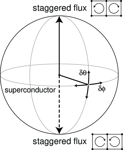
FIG. 1.: The quantization axis $\textstyle I$ in the SU(2) gauge theory. The north and south poles correspond to the staggered flux phases with shifted orbital current patterns. All points on the equators are equivalent and correspond to the $d$-wave superconductor. In the superconducting state one particular direction is chosen on the equator. There are two important collective modes. The $\theta$ modes correspond to fluctuations in the polar angle $\delta\theta$ and the $\phi$ gauge mode to a spatially varying fluctuation in $\delta\phi$.

It is useful to rotate the configuration specified by Eqs.(32) and (33) back to the radial gauge. We obtain

$${\tilde{U}}_{ij}^{d}=g_{i}^{\prime\dagger}U_{ij}^{SF}e^{ia_{ij}^{3}\tau^{3}}g_{j}^{\prime}\,\,\,.$$ (53)

The advantage of the radial gauge is two-fold. The electron operator $c_{i\sigma}=r_{0}f_{i\sigma}$ and we can consider ${\tilde{U}}_{ij}^{d}$ as the effective Hamiltonian for electron quasiparticles. At the same time, we can now make contact with the fluctuation of the $U_{ij}$ matrix in the last section and interpret the numerical results.

Equation (35) can be explicitly evaluated for arbitrary $\theta$, $\phi$ and $\alpha$ and $a^{3}_{ij}$, resulting in

$$\tilde{U}_{ij}^{d}=\pmatrix{\hat{U}_{11}^{d}e^{-i(\alpha_{i}-\alpha_{j})}&\hat{U}_{12}^{d}e^{-i(\alpha_{i}+\alpha_{j})}\cr\hat{U}_{21}^{d}e^{i(\alpha_{i}+\alpha_{j})}&\hat{U}_{22}^{d}e^{i(\alpha_{i}-\alpha_{j})}}.$$ (54)

The overall phase $\alpha_{i}$ enters the effective hopping $\tilde{U}_{22}^{d}$ and effective pairing $\tilde{U}_{12}^{d}$ in the expected way, and $\hat{U}^{d}_{ij}$ is the $\alpha_{i}=0$ limit given by ref. [27].

$${\hat{U}}_{ij}^{d} = -{\tilde{\chi}}_{ij}\left[\tau^{3}\cos{\theta_{i}-\theta_{j}\over 2}+(-1)^{i_{x}+i_{y}}\tau^{2}\sin{\theta_{i}-\theta_{j}\over 2}\right]$$ (56)

$$-{\tilde{\Delta}}_{ij}\left[\rule{0.0pt}{10.84006pt}i(-1)^{i_{x}+i_{y}}\cos{\theta_{i}+\theta_{j}\over 2}-\tau^{1}\sin{\theta_{i}+\theta_{j}\over 2}\right]$$

where

$${\tilde{\chi}}_{ij} = A\cos\tilde{\Phi}_{ij}$$ (57)

$${\tilde{\Delta}}_{ij} = A\eta_{j-i}\sin\tilde{\Phi}_{ij}$$ (58)

$${\tilde{\Phi}}_{ij} = \Phi_{0}+(-1)^{i_{x}+j_{y}}v_{ij}$$ (59)

and

$$v_{ij}={\phi_{i}-\phi_{j}\over 2}-a_{ij}^{3}\,\,\,.$$ (60)

Note that the only dependence on $\phi_{i}$, $\phi_{j}$ is via the gauge invariant combination $v_{ij}$, which has the interpretation of the gauge current. Furthermore, for $\theta_{i}=\theta_{j}={\pi\over 2}$, we see from Eqs.(36) and (37) that ${\tilde{\chi}}_{ij}e^{i(\alpha_{i}-\alpha_{j})}$ and ${\tilde{\Delta}}_{ij}e^{-i(\alpha_{i}+\alpha_{j})}$ play the role of the effective hopping and pairing parameters. Thus fluctuations in $\phi_{i}$ leading to nonzero $v_{ij}$ means a fluctuation in the amplitude of ${\tilde{\chi}}_{ij}$ and ${\tilde{\Delta}}_{ij}$ in such a way that $|{\tilde{\chi}}_{ij}|^{2}+|{\tilde{\Delta}}_{ij}|^{2}=A^{2}$ is fixed. This is shown in Fig.2.

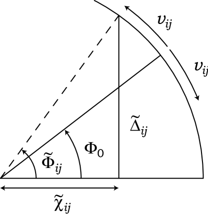
FIG. 2.: Geometrical interpretation of the fluctuation of $v_{ij}$. The angle $\tilde{\chi}_{ij}$ [given by Eq.(38)] is modulated around the flux $\Phi_{0}$ in a staggered manner, in such a way that the hopping amplitude $\tilde{\Phi}_{ij}$ and the pairing amplitude $\tilde{\Delta}_{ij}$ are modulated, also in a staggered manner.

To make contact with the collective modes, we write $\theta_{i}={\pi\over 2}+\delta\theta_{i}$ and expand Eqs.(36,37) to first order in $\delta\theta_{i}$, $v_{ij}$ and $\alpha_{i}$.

$${\tilde{U}}_{ij}^{d}-U_{ij}^{d} = -\chi_{0}\tau^{2}{(-1)^{i_{x}+i_{y}}\over 2}(\delta\theta_{i}-\delta\theta_{j})+i\Delta_{0}\eta_{\mu}{(-1)^{i_{x}+i_{y}}\over 2}(\delta\theta_{i}+\delta\theta_{j})$$ (64)

$$+\left(\chi_{0}\tau^{1}+\Delta_{0}\eta_{\mu}\tau^{3}\right){(-1)^{i_{x}+i_{y}}\over 2}v_{ij}$$

$$+i{1\over 2}\chi_{0}(\alpha_{i}-\alpha_{j})$$

$$+{1\over 2}\Delta_{0}\eta_{\mu}\tau^{2}(\alpha_{i}+\alpha_{j})$$

where $j=i+\mu$, $\mu=\hat{x},\hat{y}$.

Equation (40) is a main result of this section, as it allows us to interpret the collective modes when compared with Eq.(26). It predicts the location in momentum space of the soft collective modes and gives the eigenvectors. We classify the modes as follows:

$$\mbox{\rm{uniform}}\rule{3.61371pt}{0.0pt}\alpha:\alpha_{i} \approx \alpha_{u},$$ (65)

$$\mbox{\rm{staggered}}\rule{3.61371pt}{0.0pt}\alpha:\alpha_{i} \approx \alpha_{s}(-1)^{i_{x}+i_{y}},$$ (66)

$$\mbox{\rm{uniform}}\rule{3.61371pt}{0.0pt}\theta:\theta_{i} \approx \theta_{u},$$ (67)

$$\mbox{\rm{staggered}}\rule{3.61371pt}{0.0pt}\theta:\theta_{i} \approx \theta_{s}(-1)^{i_{x}+i_{y}},$$ (68)

We consider $\alpha_{u}$, $\alpha_{s}$, $\theta_{u}$, $\theta_{s}$ and $v_{i,i+\mu}(\mu=x,y)$ as six slowly varying variables and the first four variables are defined as follows

$${1\over 2}\left(\alpha_{i}+\alpha_{j}\right) = \alpha_{u}$$ (69)

$${1\over 2}\left(\alpha_{i}-\alpha_{j}\right) = (-1)^{i_{x}+i_{y}}\alpha_{s}$$ (70)

$${1\over 2}\left(\theta_{i}+\theta_{j}\right) = \theta_{u}$$ (71)

$${1\over 2}\left(\theta_{i}-\theta_{j}\right) = (-1)^{i_{x}+i_{y}}\theta_{s}$$ (72)

Substitution into Eq.(40) and comparison with Eq.(26) show that at $\mathchoice{{\hbox{\boldmath$\displaystyle q$}}}{{\hbox{\boldmath$\textstyle q$}}}{{\hbox{\boldmath$\scriptstyle q$}}}{{\hbox{\boldmath$\scriptscriptstyle q$}}}=0$, we can identify the following collective modes and their eigenvectors.

$$\begin{array}[]{lcc}\mbox{\rm{Goldstone mode:}}&\alpha_{u}&,\rule{10.84006pt}{0.0pt}U_{x}^{2}-U_{y}^{2}\\ \mbox{\rm{internal phase mode:}}&\theta_{s}&,\rule{10.84006pt}{0.0pt}U_{x}^{2}+U_{y}^{2}\end{array}$$ (73)

At $\mathchoice{{\hbox{\boldmath$\displaystyle q$}}}{{\hbox{\boldmath$\textstyle q$}}}{{\hbox{\boldmath$\scriptstyle q$}}}{{\hbox{\boldmath$\scriptscriptstyle q$}}}=(\pi,\pi)$ we pick out the coefficients of $(-1)^{i_{x}+i_{y}}$ and identify the following modes and corresponding eigenvectors.

$$\begin{array}[]{lllc}\theta\,\,\,\mbox{\rm{mode:}}&\theta_{u}&,\rule{10.84006pt}{0.0pt}U_{x}^{0}-U_{y}^{0}&\\ \phi\,\,\,\mbox{\rm{gauge\,\,mode:}}&v_{i,i+\mu}&,\rule{10.84006pt}{0.0pt}\chi_{0}U_{x}^{1}+\Delta_{0}U_{x}^{3}&,\rule{10.84006pt}{0.0pt}\chi_{0}U_{y}^{1}-\Delta_{0}U_{y}^{3}\\ \chi\,\,\,\mbox{\rm{mode:}}&\alpha_{s}&,\rule{10.84006pt}{0.0pt}U_{x}^{0}+U_{y}^{0}&\end{array}$$ (74)

The notation $aU_{x}^{\alpha}+bU_{y}^{\beta}$ means that each component of the eigenvector is $\left(\delta U_{x}^{\alpha}=a,\delta U_{y}^{\beta}=b\right)$, etc.in Eq.(26) The nature of the collective modes are readily identified from their eigenvectors. Two of these modes were known before. The Goldstone mode $\alpha_{u}$ is the standard one associated with the phase $\alpha_{u}$ of the superconducting order parameter $\Delta_{\mu}e^{-i2\alpha_{u}}$. The $\theta_{s}$ mode corresponds to the out-of-phase oscillation of the phase of the superconducting order parameter in the $x$ and $y$ directions, $|\Delta_{x}|e^{-i2\varphi_{x}}$ and $|\Delta_{y}|e^{-i2\varphi_{y}}$, such that $\theta_{s}={1\over 2}(\varphi_{x}-\varphi_{y})$. This is a property of any $d$-wave superconductor and is labelled the internal phase mode.

The $\alpha_{s}$ mode corresponds to the fluctuation in the phase of $\chi_{ij}$. In BCS theory the hopping term is fixed and not allowed to fluctuate. So this is a new degree of freedom special to the gauge theory. The slowly varying phase of $\chi_{ij}$ plays the role of the spatial component of the gauge field in the U(1) gauge theory.[20] This appears as a collective mode at $\mathchoice{{\hbox{\boldmath$\displaystyle q$}}}{{\hbox{\boldmath$\textstyle q$}}}{{\hbox{\boldmath$\scriptstyle q$}}}{{\hbox{\boldmath$\scriptscriptstyle q$}}}=(\pi,\pi)$. We shall see that just as in the U(1) theory, the $\alpha_{s}$ mode plays the crucial role in producing the correct answer for the superfluid stiffness $\rho_{s}=x$.

The new modes that are of greatest interest to us in this paper are the $\theta$ mode and the $\phi$ gauge modes. These will be discussed in greater detail later.

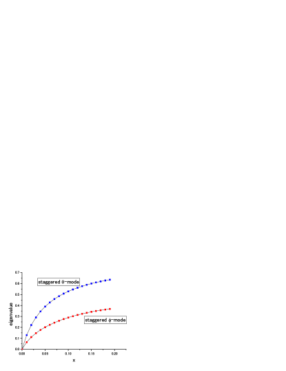
FIG. 3.: The eigenvalues at $\mathchoice{{\hbox{\boldmath$\displaystyle q$}}}{{\hbox{\boldmath$\textstyle q$}}}{{\hbox{\boldmath$\scriptstyle q$}}}{{\hbox{\boldmath$\scriptscriptstyle q$}}}=(0,0)$ and $\omega=0$ of the $9\times 9$ matrix which describes fluctuations about the mean field as a function of doping $x$. Shown are the eigenvalues which vanish as $x\rightarrow 0$. The eigenvalues are given in units of ${\tilde{J}}$. In addition to the Goldstone mode corresponding to superconducting phase fluctuations which has zero eigenvalue for all $x$ (not shown), we find the staggered $\theta$ mode [called internal phase mode in Eq.(43)] and a continuation of the transverse $\phi$-gauge mode from $\mathchoice{{\hbox{\boldmath$\displaystyle q$}}}{{\hbox{\boldmath$\textstyle q$}}}{{\hbox{\boldmath$\scriptstyle q$}}}{{\hbox{\boldmath$\scriptscriptstyle q$}}}=(\pi,\pi)$.

Now we compare our analysis with numerical results described in the last section. In Figs.3 and 4 we plot all the eigenvalues of the $9\times 9$ matrix which vanishes at $x=0$ as a function of $x$ at $\omega=0$ and at $\mathchoice{{\hbox{\boldmath$\displaystyle q$}}}{{\hbox{\boldmath$\textstyle q$}}}{{\hbox{\boldmath$\scriptstyle q$}}}{{\hbox{\boldmath$\scriptscriptstyle q$}}}=0$ and $\mathchoice{{\hbox{\boldmath$\displaystyle q$}}}{{\hbox{\boldmath$\textstyle q$}}}{{\hbox{\boldmath$\scriptstyle q$}}}{{\hbox{\boldmath$\scriptscriptstyle q$}}}=(\pi,\pi)$, respectively. They can all be identified with our classification. At $\mathchoice{{\hbox{\boldmath$\displaystyle q$}}}{{\hbox{\boldmath$\textstyle q$}}}{{\hbox{\boldmath$\scriptstyle q$}}}{{\hbox{\boldmath$\scriptscriptstyle q$}}}=0$ the Goldstone mode has zero eigenvalue for all $x$ as expected. The internal phase mode rises rapidly with increasing $x$. In addition, we find a mode with an eigenvector that corresponds to the continuation of the transverse $\phi$ gauge mode we find at $\mathchoice{{\hbox{\boldmath$\displaystyle q$}}}{{\hbox{\boldmath$\textstyle q$}}}{{\hbox{\boldmath$\scriptstyle q$}}}{{\hbox{\boldmath$\scriptscriptstyle q$}}}=(\pi,\pi)$ to $\mathchoice{{\hbox{\boldmath$\displaystyle q$}}}{{\hbox{\boldmath$\textstyle q$}}}{{\hbox{\boldmath$\scriptstyle q$}}}{{\hbox{\boldmath$\scriptscriptstyle q$}}}=0$.

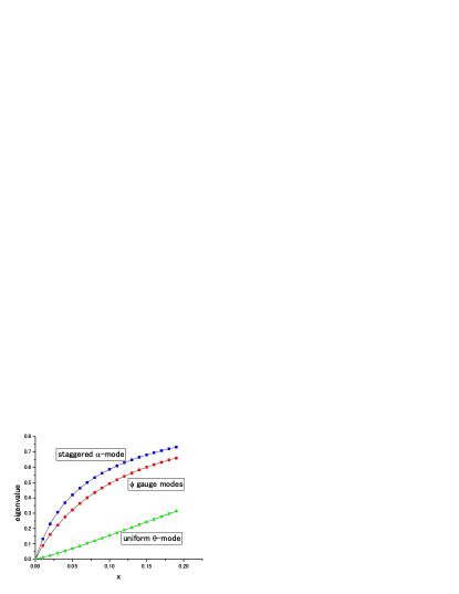
FIG. 4.: Same as Fig.3 but at $\mathchoice{{\hbox{\boldmath$\displaystyle q$}}}{{\hbox{\boldmath$\textstyle q$}}}{{\hbox{\boldmath$\scriptstyle q$}}}{{\hbox{\boldmath$\scriptscriptstyle q$}}}=(\pi,\pi)$. We find the uniform $\theta$ mode, two degenerate $\phi$ modes, and a staggered $\alpha$ mode [called the $\chi$ mode in Eq.(44)].

At $\mathchoice{{\hbox{\boldmath$\displaystyle q$}}}{{\hbox{\boldmath$\textstyle q$}}}{{\hbox{\boldmath$\scriptstyle q$}}}{{\hbox{\boldmath$\scriptscriptstyle q$}}}=(\pi,\pi)$ we find the $\theta$ mode and the two $\phi$ gauge modes (transverse and longitudinal) which are degenerate. In addition we find the $\chi$ mode. The vanishing of the eigenvalues of all these modes at $x=0$ is a consequence of the SU(2) symmetry. However, as we discussed before, even if $|\chi|\neq|\Delta|$, as long as $x=0$ the $\theta$ mode still has zero eigenvalue and the $\phi$ gauge modes are protected by the residual U(1) symmetry. These modes are gapped only by the boson condensation.

We should mention that in addition to these soft modes, we found two unstable eigenstates for small $x$. If we use in Eq. (21) ${\tilde{t}}/{\tilde{J}}=16/3$, i.e., ${\tilde{t}}/J=2$ and $t^{\prime}=-0.5t$, which generates a realistic Fermi surface, the eigenvalue corresponding to $r_{0}$ fluctuation is negative for $x<0.084$. Since $r_{0}$ corresponds to hole density, this signals an instability to phase separation. This instability is easily suppressed by long range interaction and is largely decoupled from the modes of interest. A second instability occurs for $x<x_{c}$ near $\mathchoice{{\hbox{\boldmath$\displaystyle q$}}}{{\hbox{\boldmath$\textstyle q$}}}{{\hbox{\boldmath$\scriptstyle q$}}}{{\hbox{\boldmath$\scriptscriptstyle q$}}}=(0,\pi)$ and $(\pi,0)$. The eigenvector corresponds to amplitude fluctuations in $|\chi|^{2}+|\Delta|^{2}$ which we identify as instability to columnar dimer formation. This instability is well known for $x=0$ and can be suppressed by bi-quadratic terms.[28] For the parameters mentioned above, we find $x_{c}=0.087$. Most of our detailed numerical results are for $x>x_{c}$. Furthermore these two modes are mostly decoupled from the low lying modes in Eq.(41), and does not disturb their behavior in the limit $x\to 0$ discussed in the followings.

We next discuss in greater detail the $\theta$ and the $\phi$ gauge modes. As seen in Fig.1, the $\theta$ mode is a fluctuation of $\textstyle I$ towards the north and south poles, and describes the admixture of the $s$-flux phase. From Eq.(37) we see that $\theta_{u}$ generates a staggered imaginary part to the hopping matrix elements which will produce staggered orbital currents. Thus the physical manifestation of the $\theta$ mode is staggered orbital current fluctuations. The softness of the $\theta$ mode means that it is readily excited by thermal or quantum fluctuations. This is clearly related to the strong staggered orbital current fluctuations found in the projected $d$-wave superconductor wavefunction.[17] The energy cost is low because the $s$-flux and the $d$-wave superconductor are almost degenerate in energy. The energy difference arises only because $\mathchoice{{\hbox{\boldmath$\displaystyle a$}}}{{\hbox{\boldmath$\textstyle a$}}}{{\hbox{\boldmath$\scriptstyle a$}}}{{\hbox{\boldmath$\scriptscriptstyle a$}}}_{0}$ is different in the two states. At the mean field level, the energy difference comes from the Fermi pockets and is proportional to $x^{2}$. However, we find that after integrating out $\mathchoice{{\hbox{\boldmath$\displaystyle a$}}}{{\hbox{\boldmath$\textstyle a$}}}{{\hbox{\boldmath$\scriptstyle a$}}}{{\hbox{\boldmath$\scriptscriptstyle a$}}}_{0}$, the energy cost increases, apparently due to the enforcement of the constraint and the eigenvalue shown in Fig.3 is linear in $x$. We have also computed the eigenvalues for finite $\omega$. It should be noted that the $9\times 9$ matrix is not Hermitian for finite $\omega_{m}$(Matsubara frequency). Then we make the analytic continuation as $i\omega_{m}\to\omega+i\delta$ with infinitestimal $\delta>0$. This $\delta$ can be neglected outside of the particle-hole continuum, and in this case the $9\times 9$ matrix is Hermitian and its eigenvalues are real. We will present below the results for $(\mathchoice{{\hbox{\boldmath$\displaystyle q$}}}{{\hbox{\boldmath$\textstyle q$}}}{{\hbox{\boldmath$\scriptstyle q$}}}{{\hbox{\boldmath$\scriptscriptstyle q$}}},\omega)$ outside of the particle-hole continuum. We found that the eigenvalue can be fitted by $ax-{b\over x}\omega^{2}-{c\over x}{\bf k}^{2}$ for small $\omega$ and $\mathchoice{{\hbox{\boldmath$\displaystyle k$}}}{{\hbox{\boldmath$\textstyle k$}}}{{\hbox{\boldmath$\scriptstyle k$}}}{{\hbox{\boldmath$\scriptscriptstyle k$}}}=\mathchoice{{\hbox{\boldmath$\displaystyle q$}}}{{\hbox{\boldmath$\textstyle q$}}}{{\hbox{\boldmath$\scriptstyle q$}}}{{\hbox{\boldmath$\scriptscriptstyle q$}}}-(\pi,\pi)$. The inverse $x$ dependence of the coefficient might be surprising but the $\omega^{2}$ and $\bf k$ region shrinks as $x$ becomes small, so that the $x=0$ limit is smoothly attained. Furthermore, the negative coefficient of $\mathchoice{{\hbox{\boldmath$\displaystyle k$}}}{{\hbox{\boldmath$\textstyle k$}}}{{\hbox{\boldmath$\scriptstyle k$}}}{{\hbox{\boldmath$\scriptscriptstyle k$}}}^{2}$ indicates that the eigenvalue has a local maximum at $\mathchoice{{\hbox{\boldmath$\displaystyle q$}}}{{\hbox{\boldmath$\textstyle q$}}}{{\hbox{\boldmath$\scriptstyle q$}}}{{\hbox{\boldmath$\scriptscriptstyle q$}}}=(\pi,\pi)$. A plausible dependence is $\sqrt{(ax)^{2}-b^{\prime}\omega^{2}-c^{\prime}{\bf k}^{2}}$, which is reduced to the above form in the limit $|\omega|,|{\bf k}|<<x$. Back to the Matsubara frequency, the suggested effective action for the $\theta$ mode is

$$S_{\theta}=\sum_{\mathchoice{{\hbox{\boldmath$\displaystyle k$}}}{{\hbox{\boldmath$\textstyle k$}}}{{\hbox{\boldmath$\scriptstyle k$}}}{{\hbox{\boldmath$\scriptscriptstyle k$}}},\omega_{m}}\sqrt{(ax)^{2}+b^{\prime}\omega_{m}^{2}-c^{\prime}{\bf k}^{2}}|\theta(\mathchoice{{\hbox{\boldmath$\displaystyle k$}}}{{\hbox{\boldmath$\textstyle k$}}}{{\hbox{\boldmath$\scriptstyle k$}}}{{\hbox{\boldmath$\scriptscriptstyle k$}}},\omega_{m})|^{2}$$ (75)

in the region $|\omega_{m}|,|{\bf k}|<<x$. The small energy gap $ax$ leads to a strong spectral weight. This is confirmed by direct numerical calculations in the next section. Here it is interesting to compare these results with the SU(2) formalism with those in the U(1) where only $a_{0}^{3}$ is integrated over. The suggested action in this case is

$$S^{U(1)}_{\theta}=\sum_{\mathchoice{{\hbox{\boldmath$\displaystyle k$}}}{{\hbox{\boldmath$\textstyle k$}}}{{\hbox{\boldmath$\scriptstyle k$}}}{{\hbox{\boldmath$\scriptscriptstyle k$}}},\omega_{m}}\left[(ax)^{2}+b^{\prime\prime}\omega_{m}^{2}+c^{\prime\prime}x{\bf k}^{2}\right]|\theta(\mathchoice{{\hbox{\boldmath$\displaystyle k$}}}{{\hbox{\boldmath$\textstyle k$}}}{{\hbox{\boldmath$\scriptstyle k$}}}{{\hbox{\boldmath$\scriptscriptstyle k$}}},\omega_{m})|^{2}.$$ (76)

Therefore it is evident that the SU(2) symmetry leads to quite different $x$-dependence in the limit $x\to 0$.

To investigate the $\phi$ gauge modes we first discuss $x=0$. The mean field solution is the $\pi$-flux phase where the fermions obey the Dirac spectra with nodes at $(\pm{\pi\over 2},\pm{\pi\over 2})$. After integrating out the fermions, it is known that the effective gauge field action is purely transverse and given by[30]

$$S_{\phi}=\sum_{\mathchoice{{\hbox{\boldmath$\displaystyle k$}}}{{\hbox{\boldmath$\textstyle k$}}}{{\hbox{\boldmath$\scriptstyle k$}}}{{\hbox{\boldmath$\scriptscriptstyle k$}}},\omega_{m}}\alpha_{0}\sqrt{\mathchoice{{\hbox{\boldmath$\displaystyle k$}}}{{\hbox{\boldmath$\textstyle k$}}}{{\hbox{\boldmath$\scriptstyle k$}}}{{\hbox{\boldmath$\scriptscriptstyle k$}}}^{2}+\omega_{m}^{2}}\left(\delta_{\mu\nu}-{\mathchoice{{\hbox{\boldmath$\displaystyle k$}}}{{\hbox{\boldmath$\textstyle k$}}}{{\hbox{\boldmath$\scriptstyle k$}}}{{\hbox{\boldmath$\scriptscriptstyle k$}}}_{\mu}\mathchoice{{\hbox{\boldmath$\displaystyle k$}}}{{\hbox{\boldmath$\textstyle k$}}}{{\hbox{\boldmath$\scriptstyle k$}}}{{\hbox{\boldmath$\scriptscriptstyle k$}}}_{\nu}\over\mathchoice{{\hbox{\boldmath$\displaystyle k$}}}{{\hbox{\boldmath$\textstyle k$}}}{{\hbox{\boldmath$\scriptstyle k$}}}{{\hbox{\boldmath$\scriptscriptstyle k$}}}^{2}}\right)a_{\mu}(\mathchoice{{\hbox{\boldmath$\displaystyle k$}}}{{\hbox{\boldmath$\textstyle k$}}}{{\hbox{\boldmath$\scriptstyle k$}}}{{\hbox{\boldmath$\scriptscriptstyle k$}}},\omega_{m})a_{\nu}(\mathchoice{{\hbox{\boldmath$\displaystyle k$}}}{{\hbox{\boldmath$\textstyle k$}}}{{\hbox{\boldmath$\scriptstyle k$}}}{{\hbox{\boldmath$\scriptscriptstyle k$}}},-\omega_{m})$$ (77)

where ${\mathchoice{{\hbox{\boldmath$\displaystyle a$}}}{{\hbox{\boldmath$\textstyle a$}}}{{\hbox{\boldmath$\scriptstyle a$}}}{{\hbox{\boldmath$\scriptscriptstyle a$}}}}_{\mu}$ is the continuum version of $a_{i,i+\mu}$ and $\textstyle k$ is measured relative to $(\pi,\pi)$. We confirm this by computing the eigenvalues for $x=0$ at finite $\mathchoice{{\hbox{\boldmath$\displaystyle q$}}}{{\hbox{\boldmath$\textstyle q$}}}{{\hbox{\boldmath$\scriptstyle q$}}}{{\hbox{\boldmath$\scriptscriptstyle q$}}}=(1.03\pi,\pi)$. The transverse mode behaves as $\sqrt{k^{2}+\omega_{m}^{2}}$ as expected while the longitudinal mode is exactly zero for all $\omega_{m}$. This is because the longitudinal mode is pure gauge $(\mathchoice{{\hbox{\boldmath$\displaystyle a$}}}{{\hbox{\boldmath$\textstyle a$}}}{{\hbox{\boldmath$\scriptstyle a$}}}{{\hbox{\boldmath$\scriptscriptstyle a$}}}_{\mu}=\mathchoice{{\hbox{\boldmath$\displaystyle\nabla$}}}{{\hbox{\boldmath$\textstyle\nabla$}}}{{\hbox{\boldmath$\scriptstyle\nabla$}}}{{\hbox{\boldmath$\scriptscriptstyle\nabla$}}}_{\mu}\phi)$ and is not a real degree of freedom. In constrast, if we worked with the U(1) formulation [Eq.(7)], we find that the longitudinal mode has eigenvalue close to $|\omega|$. Thus the addition of the $a_{0}^{1}$ and $a_{0}^{2}$ in the SU(2) formulation is crucial. Otherwise we would have gotten a spurious collective mode. This is a dramatic illustration of the advantage of the SU(2) formulation, if one is interested in obtaining meaningful results which are smoothly connected to the undoped case. For finite $x$ we see from Fig.3 that the eigenvalue increases linearly with $x$ for small $x$. A reasonable approximate for the transverse mode is $\left[\mbox{\rm for}\,\,\,\mathchoice{{\hbox{\boldmath$\displaystyle k$}}}{{\hbox{\boldmath$\textstyle k$}}}{{\hbox{\boldmath$\scriptstyle k$}}}{{\hbox{\boldmath$\scriptscriptstyle k$}}}=\mathchoice{{\hbox{\boldmath$\displaystyle q$}}}{{\hbox{\boldmath$\textstyle q$}}}{{\hbox{\boldmath$\scriptstyle q$}}}{{\hbox{\boldmath$\scriptscriptstyle q$}}}-(\pi,\pi)\right]$

$$S^{{\rm transverse}}_{\phi}=\sum_{\mathchoice{{\hbox{\boldmath$\displaystyle k$}}}{{\hbox{\boldmath$\textstyle k$}}}{{\hbox{\boldmath$\scriptstyle k$}}}{{\hbox{\boldmath$\scriptscriptstyle k$}}},\omega_{m}}\left(\alpha_{0}\sqrt{(a_{\varphi}x)^{2}+\mathchoice{{\hbox{\boldmath$\displaystyle k$}}}{{\hbox{\boldmath$\textstyle k$}}}{{\hbox{\boldmath$\scriptstyle k$}}}{{\hbox{\boldmath$\scriptscriptstyle k$}}}^{2}+\omega_{m}^{2}}\rule{3.61371pt}{0.0pt}\right)\left(\delta_{\mu\nu}-{\mathchoice{{\hbox{\boldmath$\displaystyle k$}}}{{\hbox{\boldmath$\textstyle k$}}}{{\hbox{\boldmath$\scriptstyle k$}}}{{\hbox{\boldmath$\scriptscriptstyle k$}}}_{\mu}\mathchoice{{\hbox{\boldmath$\displaystyle k$}}}{{\hbox{\boldmath$\textstyle k$}}}{{\hbox{\boldmath$\scriptstyle k$}}}{{\hbox{\boldmath$\scriptscriptstyle k$}}}_{\nu}\over\mathchoice{{\hbox{\boldmath$\displaystyle k$}}}{{\hbox{\boldmath$\textstyle k$}}}{{\hbox{\boldmath$\scriptstyle k$}}}{{\hbox{\boldmath$\scriptscriptstyle k$}}}^{2}}\right)v_{\mu}(\mathchoice{{\hbox{\boldmath$\displaystyle k$}}}{{\hbox{\boldmath$\textstyle k$}}}{{\hbox{\boldmath$\scriptstyle k$}}}{{\hbox{\boldmath$\scriptscriptstyle k$}}},\omega_{m})v_{\nu}(\mathchoice{{\hbox{\boldmath$\displaystyle k$}}}{{\hbox{\boldmath$\textstyle k$}}}{{\hbox{\boldmath$\scriptstyle k$}}}{{\hbox{\boldmath$\scriptscriptstyle k$}}},\omega_{m})$$ (78)

where

$$\mathchoice{{\hbox{\boldmath$\displaystyle v$}}}{{\hbox{\boldmath$\textstyle v$}}}{{\hbox{\boldmath$\scriptstyle v$}}}{{\hbox{\boldmath$\scriptscriptstyle v$}}}_{\mu}={1\over 2}\mathchoice{{\hbox{\boldmath$\displaystyle\nabla$}}}{{\hbox{\boldmath$\textstyle\nabla$}}}{{\hbox{\boldmath$\scriptstyle\nabla$}}}{{\hbox{\boldmath$\scriptscriptstyle\nabla$}}}_{\mu}\phi-\mathchoice{{\hbox{\boldmath$\displaystyle a$}}}{{\hbox{\boldmath$\textstyle a$}}}{{\hbox{\boldmath$\scriptstyle a$}}}{{\hbox{\boldmath$\scriptscriptstyle a$}}}_{\mu}$$ (79)

is the continuum limit of $v_{i,i+\mu}$ and $\alpha_{0}$ parameterizes the spectral weight. Thus we expect the transverse mode to show an edge singularity starting at $\omega=\sqrt{(a_{\phi}x)^{2}+\mathchoice{{\hbox{\boldmath$\displaystyle k$}}}{{\hbox{\boldmath$\textstyle k$}}}{{\hbox{\boldmath$\scriptstyle k$}}}{{\hbox{\boldmath$\scriptscriptstyle k$}}}^{2}}$. In Fig.5 we show the eigenvalues of the $\phi$ gauge modes as function of $(q_{x}-\pi)/\pi$ at $q_{y}=\pi$ and $\omega_{m}=0$, which shows the expected dependence on $q_{x}-\pi$ from eq.(48) for transverse mode.

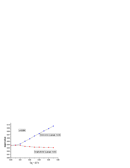
FIG. 5.: The eigenvalue (in units of ${\tilde{J}}$) of the transverse and longitudinal $\phi$ gauge mode as a function of $k_{x}/\pi=(q_{x}-\pi)/\pi$ with $q_{y}=\pi$ and $\omega_{m}=0$ for $x=0.004$. They show the expected behavior for small $x$ and $\textstyle q$ near $(\pi,\pi)$ because when $x=0$ and $\omega_{m}=0$, the transverse mode should be linear in $|\mathchoice{{\hbox{\boldmath$\displaystyle k$}}}{{\hbox{\boldmath$\textstyle k$}}}{{\hbox{\boldmath$\scriptstyle k$}}}{{\hbox{\boldmath$\scriptscriptstyle k$}}}|$ and the longitudinal mode should be zero for all $\textstyle q$ and $\omega_{m}$.

At finite $x$ the longitudinal mode becomes a real degree of freedom due to the breaking of the residual U(1) symmetry. At $\omega_{m}=0$ and $\mathchoice{{\hbox{\boldmath$\displaystyle q$}}}{{\hbox{\boldmath$\textstyle q$}}}{{\hbox{\boldmath$\scriptstyle q$}}}{{\hbox{\boldmath$\scriptscriptstyle q$}}}=(\pi,\pi)$ the eigenvalue is $a_{\phi}x$, degenerate with the transverse mode. For finite $k_{x}=q_{x}-\pi$, the eigenvalue shows a slow decrease and then saturates. This is shown in Fig.5. This is to be expected as the eigenvalue is zero for all $\omega_{m}$ and $\textstyle q$ for $x=0$. As for the spectral function, we just invert the $12\times 12$ matrix numerically with $\omega_{m}\to\omega+i\delta$, and we do not have to worry about the non-Hermitian nature of the matrix, which will be shown in the next section. It is worth noting that the longitudinal gauge mode is the only mode with significant coupling to $\delta R$ and therefore to density fluctuations.

We next discuss the Goldstone mode. We expect the eigenvalue to be of the form $\rho_{s}(\mathchoice{{\hbox{\boldmath$\displaystyle\nabla\alpha$}}}{{\hbox{\boldmath$\textstyle\nabla\alpha$}}}{{\hbox{\boldmath$\scriptstyle\nabla\alpha$}}}{{\hbox{\boldmath$\scriptscriptstyle\nabla\alpha$}}})^{2}$, where $\alpha$ is the continuum limit of a slowly varying $\alpha_{u}$. We indeed verify that upon diagonalizing the $9\times 9$ matrix described in the last section, a soft eigenvalue emerges which is linear in $q^{2}$. Furthermore the coefficient $\rho_{s}$ is proportional to $x$. This is to be expected in our SU(2) formulation, as $x=0$ is an insulator. It is interesting to analyze how this result emerges. The point is that the coefficient of $(\nabla\alpha_{u})^{2}$ in the free energy computed using Eqs.(21,40) is $\rho_{f}$, which corresponds to the superfluid density of a nearly half-filled conventional superconductor, and $\rho_{f}\approx 1$. How do we obtain $\rho_{s}=x$ ? In the numerics we find that the $\rho_{s}q^{2}$ mode is a coupled mode between $\alpha_{u}$ and $\alpha_{s}$. Recall that $\alpha_{s}$ is related to the phase of $\chi_{ij}$ and may therefore be identified with the U(1) gauge field $\textstyle a$ in the U(1) formulation.[20] In that formulation the free energy in the superconducting (Bose condensed) state takes the form

$$F=\rho_{f}(\mathchoice{{\hbox{\boldmath$\displaystyle\nabla$}}}{{\hbox{\boldmath$\textstyle\nabla$}}}{{\hbox{\boldmath$\scriptstyle\nabla$}}}{{\hbox{\boldmath$\scriptscriptstyle\nabla$}}}\alpha_{u}-\mathchoice{{\hbox{\boldmath$\displaystyle a$}}}{{\hbox{\boldmath$\textstyle a$}}}{{\hbox{\boldmath$\scriptstyle a$}}}{{\hbox{\boldmath$\scriptscriptstyle a$}}})^{2}+\rho_{b}|\mathchoice{{\hbox{\boldmath$\displaystyle a$}}}{{\hbox{\boldmath$\textstyle a$}}}{{\hbox{\boldmath$\scriptstyle a$}}}{{\hbox{\boldmath$\scriptscriptstyle a$}}}|^{2}$$ (80)

where $\rho_{b}=x$ and $\rho_{f}$ is the fermion contribution to the superfluid density, which is of order unity. Upon minimizing $F$ with respect to $\textstyle a$, we arrive at the Ioffe-Larkin formula[30] $F=\rho_{s}(\nabla\alpha_{u})^{2}$ where

$$\rho_{s}={\rho_{b}\rho_{f}\over\rho_{b}+\rho_{f}}\,\,\,.$$ (81)

The screening of $\nabla\alpha_{u}$ by the gauge field $\textstyle a$ converts the fermion response $\rho_{f}$ to the physical response $\rho_{s}\approx x$. When we express Eq.(50) in matrix form we see that the free energy has diagonal contributions $\rho_{f}(\mathchoice{{\hbox{\boldmath$\displaystyle\nabla$}}}{{\hbox{\boldmath$\textstyle\nabla$}}}{{\hbox{\boldmath$\scriptstyle\nabla$}}}{{\hbox{\boldmath$\scriptscriptstyle\nabla$}}}\alpha_{u})^{2}$ and $(\rho_{f}+\rho_{b})\mathchoice{{\hbox{\boldmath$\displaystyle a$}}}{{\hbox{\boldmath$\textstyle a$}}}{{\hbox{\boldmath$\scriptstyle a$}}}{{\hbox{\boldmath$\scriptscriptstyle a$}}}^{2}$ and an off-diagonal term $-\rho_{f}\mathchoice{{\hbox{\boldmath$\displaystyle\nabla$}}}{{\hbox{\boldmath$\textstyle\nabla$}}}{{\hbox{\boldmath$\scriptstyle\nabla$}}}{{\hbox{\boldmath$\scriptscriptstyle\nabla$}}}\alpha_{u}\cdot\mathchoice{{\hbox{\boldmath$\displaystyle a$}}}{{\hbox{\boldmath$\textstyle a$}}}{{\hbox{\boldmath$\scriptstyle a$}}}{{\hbox{\boldmath$\scriptscriptstyle a$}}}$. When we examine the $9\times 9$ matrix, we find that for small $q$, $\alpha_{u}$ is only coupled to $\alpha_{s}$ and the form of the $2\times 2$ sub-matrix is just that given by the above discussion if we identify $\textstyle a$ with $\alpha_{s}$. Upon diagonalizing the $2\times 2$ matrix, the soft mode with eigenvalue $\rho_{s}q^{2}$ emerges. This simply confirms that our SU(2) formulation contains the same U(1) gauge field and the same screening mechanism is at work. One consequence of Ioffe-Larkin screening is that at finite temperature $\rho_{s}(T)=\rho_{s}(0)-Cx^{2}T$, i.e., the coefficient of the linear $T$ term is proportional to $x^{2}$. We have also verified numerically that this is the case by computing $\rho_{s}$ at finite $T$. Experimentally, there is strong evidence that the coefficient of the linear $T$ term is independent of $x$.[31] The fact that $\rho_{s}$ is proportional to $x$ can be seen more readily if we associate the phase $\alpha_{i}$ with $b_{i}$ in Eq.(13) instead of with $z_{i}$ as we have done so far. Then it is clear that for static $\alpha_{i}$, only the last term in Eq.(12) depends on $\alpha_{i}-\alpha_{j}$ and the free energy change must be proportional to $r^{2}_{0}\approx x$. Furthermore, the coupling to fermion excitations is proportional to $x$, so that the response to thermal excitations of quasiparticles is proportional to $x^{2}$. Thus Ioffe-Larkin and our fluctuation theory are in disagreement with experiment. We believe this is an indication that the fermions and bosons are confined to become electrons in the superconducting state and that confinement physics is beyond the Gaussian fluctuation considered here.

V Numerical Results for the Spectral Functions of the $\theta$ Mode and the $\phi$ Gauge Modes

As shown in Appendix A, the collective fluctuations about the saddle point is described by the quadratic form

$$S_{\mbox{\rm eff}}=X_{\alpha}\left(M_{\alpha\beta}^{J}+M_{\alpha\beta}^{F}\right)X_{\beta},\rule{6.50403pt}{0.0pt}\alpha=1...12$$ (82)

where $X_{\alpha}=\left(\delta U_{\mu}^{\ell},...,\delta R,a_{0}^{1},a_{0}^{2},a_{0}^{3}\right)$ are the 12 degrees of freedom and $M_{\alpha\beta}^{F}(\mathchoice{{\hbox{\boldmath$\displaystyle q$}}}{{\hbox{\boldmath$\textstyle q$}}}{{\hbox{\boldmath$\scriptstyle q$}}}{{\hbox{\boldmath$\scriptscriptstyle q$}}},i\omega_{m})$ are made up of fermion bubbles computed in Appendix A. Here we study the spectral functions

$$S_{A}(\mathchoice{{\hbox{\boldmath$\displaystyle q$}}}{{\hbox{\boldmath$\textstyle q$}}}{{\hbox{\boldmath$\scriptstyle q$}}}{{\hbox{\boldmath$\scriptscriptstyle q$}}},\omega)=ImC_{A}(\mathchoice{{\hbox{\boldmath$\displaystyle q$}}}{{\hbox{\boldmath$\textstyle q$}}}{{\hbox{\boldmath$\scriptstyle q$}}}{{\hbox{\boldmath$\scriptscriptstyle q$}}},i\omega_{m}\rightarrow\omega+i\eta)$$ (83)

where

$$C_{A}(\mathchoice{{\hbox{\boldmath$\displaystyle q$}}}{{\hbox{\boldmath$\textstyle q$}}}{{\hbox{\boldmath$\scriptstyle q$}}}{{\hbox{\boldmath$\scriptscriptstyle q$}}},i\omega_{m})=\langle A(\mathchoice{{\hbox{\boldmath$\displaystyle q$}}}{{\hbox{\boldmath$\textstyle q$}}}{{\hbox{\boldmath$\scriptstyle q$}}}{{\hbox{\boldmath$\scriptscriptstyle q$}}},i\omega_{m})A(\mathchoice{{\hbox{\boldmath$\displaystyle q$}}}{{\hbox{\boldmath$\textstyle q$}}}{{\hbox{\boldmath$\scriptstyle q$}}}{{\hbox{\boldmath$\scriptscriptstyle q$}}},-i\omega_{m})\rangle$$ (84)

and we focus on three cases, the $\theta$ mode $(A=\theta_{u})$, the transverse and longitudinal $\phi$ gauge modes $(A=v_{i,i+\mu})$. Using Eq.(44) these are readily expressed in terms of

$$\langle X_{\alpha}X_{\beta}\rangle=\left(M^{J}+M^{F}\right)^{-1}$$ (85)

and computed numerically. We use parameters in Eq. (21) ${\tilde{t}}/{\tilde{J}}=16/3$, i.e., ${\tilde{t}}/J=2$ and $t^{\prime}/t=-0.5$, which gives realistic fermion bandstructure and we show results for $x=0.1$. The mean field parameters are $\chi_{0}=0.376$ and $\Delta_{0}=0.255$. Note that the maximum energy gap is $E_{g}=\Delta_{\mathchoice{{\hbox{\boldmath$\displaystyle k$}}}{{\hbox{\boldmath$\textstyle k$}}}{{\hbox{\boldmath$\scriptstyle k$}}}{{\hbox{\boldmath$\scriptscriptstyle k$}}}=(\pi,\pi)}=4\Delta_{0}\tilde{J}$ We measure energy in units of $\tilde{J}$ and the lattice constant is set to unity.

It is important to note that we define the correlators in terms of the eigenvectors [(Eq.44)] which are the eigenvectors fo r $\mathchoice{{\hbox{\boldmath$\displaystyle q$}}}{{\hbox{\boldmath$\textstyle q$}}}{{\hbox{\boldmath$\scriptstyle q$}}}{{\hbox{\boldmath$\scriptscriptstyle q$}}}=(\pi,\pi)$ and $\omega_{m}=0$. Away from $(\pi,\pi)$, the overlap with the true eigenmode is modified and other modes may mix in. Furthermore, for the $\phi$-gauge modes, the assignment in Eq.(44) corresponds to “polarization” in the $\hat{x}$ and $\hat{y}$ directions, and are the appropriate longitudinal and transverse modes only for $\textstyle q$ along the $(\mathchoice{{\hbox{\boldmath$\displaystyle q$}}}{{\hbox{\boldmath$\textstyle q$}}}{{\hbox{\boldmath$\scriptstyle q$}}}{{\hbox{\boldmath$\scriptscriptstyle q$}}}_{x},\pi)$ direction. Thus the numerical results shown here should be viewed as providing a guide for the behavior of the modes near $(\pi,\pi)$. In the next section we will compute correlation functions which are experimentally observable in the entire Brillouin zone.

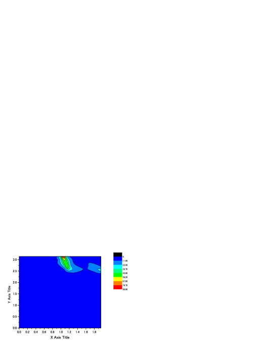
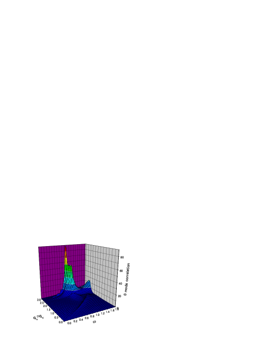
FIG. 6.: Spectral function for the $\theta$ mode for $\mathchoice{{\hbox{\boldmath$\displaystyle q$}}}{{\hbox{\boldmath$\textstyle q$}}}{{\hbox{\boldmath$\scriptstyle q$}}}{{\hbox{\boldmath$\scriptscriptstyle q$}}}=(q_{x},q_{y})$ from 0 to $(\pi,\pi)$. A contour plot and a bird’s eye view are shown. Frequency $\omega$ is in units of $\tilde{J}(={3\over 8}J)$.

Figure 6 shows the results for the $\theta$ mode $S_{\theta}(\mathchoice{{\hbox{\boldmath$\displaystyle q$}}}{{\hbox{\boldmath$\textstyle q$}}}{{\hbox{\boldmath$\scriptstyle q$}}}{{\hbox{\boldmath$\scriptscriptstyle q$}}},\omega)$ with $\textstyle q$ along the diagonal $\mathchoice{{\hbox{\boldmath$\displaystyle q$}}}{{\hbox{\boldmath$\textstyle q$}}}{{\hbox{\boldmath$\scriptstyle q$}}}{{\hbox{\boldmath$\scriptscriptstyle q$}}}_{x}=\mathchoice{{\hbox{\boldmath$\displaystyle q$}}}{{\hbox{\boldmath$\textstyle q$}}}{{\hbox{\boldmath$\scriptstyle q$}}}{{\hbox{\boldmath$\scriptscriptstyle q$}}}_{y}$ in a contour plot and also in a bird’s eye view. We see that the spectral function shows a strong peak near $\omega\approx 1.1\tilde{J}$ ($\tilde{J}$ is defined after Eq.(8) and is suggested to take the value $\tilde{J}={3\over 8}J$) which is strongly localized near $\mathchoice{{\hbox{\boldmath$\displaystyle q$}}}{{\hbox{\boldmath$\textstyle q$}}}{{\hbox{\boldmath$\scriptstyle q$}}}{{\hbox{\boldmath$\scriptscriptstyle q$}}}=(\pi,\pi)$. The spectral function disperses rapidly upwards as $\textstyle q$ deviates from $(\pi,\pi)$. The very large peak height can be anticipated from the approximate form given by Eq.(45) because the small value of the gap $ax$ gives a large spectral weight upon inversion of the effective action. The strong and narrow peak is responsible for the orbital current fluctuations in the superconducting ground state.[17]

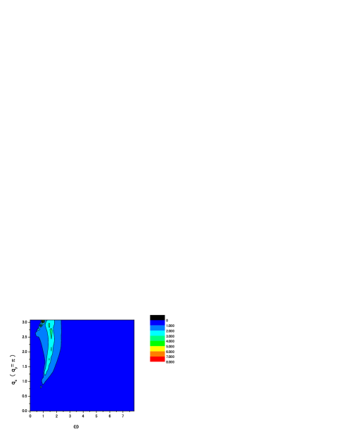
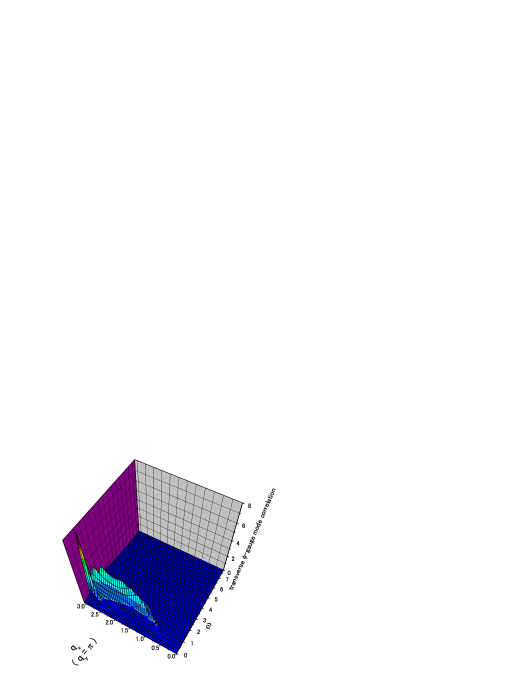
FIG. 7.: Spectral function for the transverse $\phi$ gauge mode for $\mathchoice{{\hbox{\boldmath$\displaystyle q$}}}{{\hbox{\boldmath$\textstyle q$}}}{{\hbox{\boldmath$\scriptstyle q$}}}{{\hbox{\boldmath$\scriptscriptstyle q$}}}=(q_{x},\pi)$, i.e., from $(0,\pi)$ to $(\pi,\pi)$. A contour plot and a bird’s eye view are shown. Frequency $\omega$ is in units of $\tilde{J}(={3\over 8}J)$.

Figures 7 and 8 show the transverse and longitudinal $\phi$ gauge modes along $\mathchoice{{\hbox{\boldmath$\displaystyle q$}}}{{\hbox{\boldmath$\textstyle q$}}}{{\hbox{\boldmath$\scriptstyle q$}}}{{\hbox{\boldmath$\scriptscriptstyle q$}}}=(q_{x},\pi)$. The operators are chosen to be

$$\delta\phi_{t}=\cos\Phi_{0}\delta\Delta_{y}-\sin\Phi_{0}\delta\chi_{y}$$ (86)

$$\delta\phi_{\ell}=\cos\Phi_{0}\delta\Delta_{x}+\sin\Phi_{0}\delta\chi_{x}$$ (87)

where

$$\delta\chi_{\mu}={1\over 2}(\sum_{\sigma}f^{\dagger}_{i\sigma}f_{i+\mu\sigma}+c.c.)-\chi_{0}$$ (88)

$$\delta\Delta_{\mu}={1\over 2}(f_{i\uparrow}f_{i+\mu\downarrow}-f_{i\downarrow}f_{i+\mu\uparrow}+c.c.)-\Delta_{0}\eta_{\mu}$$ (89)

are the fluctuations of the real part of $\chi_{ij}$ and $\Delta_{ij}$, respectively. Since $\chi_{0}$, $\Delta_{0}$ are real, these correspond to amplitude fluctuations. These correlators are readily related to the correlations involving $U_{\mu}^{3}$ and $U_{\mu}^{1}$, respectively. Equations (56,57) are simply the resolution of the fluctuations illustrated in Fig.2 into its components along the vertical and horizontal axes. Near $(\pi,\pi)$ the two modes are degenerate and show a peak around $\omega=1.5\tilde{J}$. The lineshape is shown in Fig.9. The mode is damped by particle-hole excitations and a sharp feature appears as the frequency drops below the particle-hole continuum. (Recall that the particle-hole continuum is set by the scale $\omega=2E_{g}\approx 2\tilde{J}$ with our parameters.) The transverse mode frequency remains low but loses spectral weight as $\textstyle q$ goes away from ${\pi,\pi}$ towards $(0,\pi)$. On the other hand, the longitudinal mode disperses upwards and gains in strength.

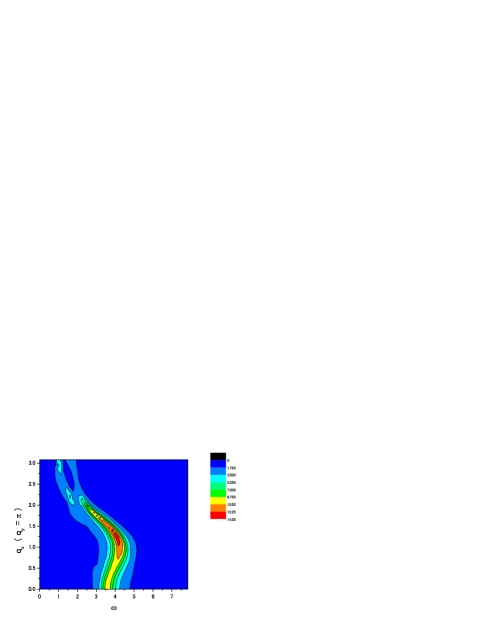
FIG. 8.: Contour plot of the spectral function for the longitudinal $\phi$ gauge mode for $\mathchoice{{\hbox{\boldmath$\displaystyle q$}}}{{\hbox{\boldmath$\textstyle q$}}}{{\hbox{\boldmath$\scriptstyle q$}}}{{\hbox{\boldmath$\scriptscriptstyle q$}}}=(q_{x},\pi)$, i.e., from $(0,\pi)$ to $(\pi,\pi)$. Frequency $\omega$ is in units of $\tilde{J}(={3\over 8}J)$.

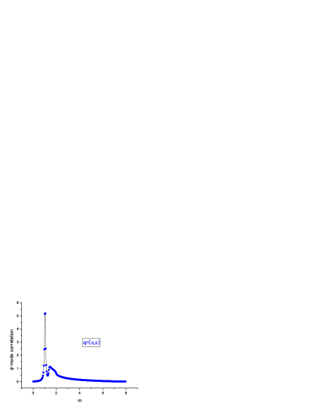
FIG. 9.: The lineshape for the $\phi$ mode at $\mathchoice{{\hbox{\boldmath$\displaystyle q$}}}{{\hbox{\boldmath$\textstyle q$}}}{{\hbox{\boldmath$\scriptstyle q$}}}{{\hbox{\boldmath$\scriptscriptstyle q$}}}=(\pi,\pi)$. Frequency $\omega$ is in units of $\tilde{J}(={3\over 8}J)$.

Finally we discuss another important mode which is closely related to the $\phi$ gauge mode. It is the fluctuation of the amplitude $A_{\mu}=\sqrt{|\chi_{i,i+\mu}|^{2}+|\Delta_{i,i+\mu}|^{2}}$ and is parametrized by

$$\delta A_{\mu}=\sin\Phi_{0}\delta\Delta_{\mu}+\cos\Phi_{0}\delta\chi_{\mu}\,\,\,.$$ (90)

Unlike the modes discussed so far, the amplitude mode has finite eigenvalue in the $x=0$ limit. However, for $x\approx 0.1$ the $\omega_{m}=0$ eigenvalue for the $\phi$ mode has reached the value 0.493, quite close to the amplitude mode eigenvalue of 0.669. As seen from Eqs.(56,57,60) both these modes involve the fluctuation of the amplitudes of $\chi$ and $\Delta$, and they will admix for finite frequency. This complicates the interpretation of these collective modes. In contrast, the eigenvalue of the $\theta$ mode is quite low at 0.155 and its interpretation as a collective mode is more clear. In Fig.10 we show the spectral function for the ampltidue mode at $\mathchoice{{\hbox{\boldmath$\displaystyle q$}}}{{\hbox{\boldmath$\textstyle q$}}}{{\hbox{\boldmath$\scriptstyle q$}}}{{\hbox{\boldmath$\scriptscriptstyle q$}}}=(\pi,\pi)$.

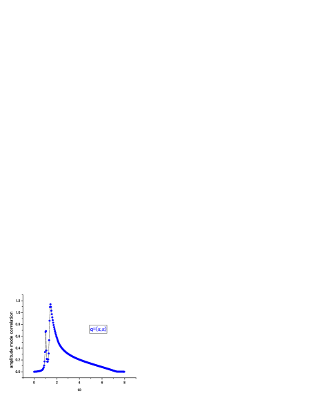
FIG. 10.: Spectral function of the amplitude mode at $\mathchoice{{\hbox{\boldmath$\displaystyle q$}}}{{\hbox{\boldmath$\textstyle q$}}}{{\hbox{\boldmath$\scriptstyle q$}}}{{\hbox{\boldmath$\scriptscriptstyle q$}}}=(\pi,\pi)$.

VI Experimental Observation of the Collective Modes

Finally, we discuss possible experimental consequences of these collective modes. As discussed earlier, the $\theta$ mode produces staggered orbital currents. These in turn generate a physical magnetic field which is staggered and which is, in principle, observable by inelastic neutron scattering. Here we compute the scattering cross-section. The neutron scattering by orbital currents has been considered by Hsu et al.[32] and we follow their discussion. We find that

$${d\sigma\over d\Omega d{\mathchoice{{\hbox{\boldmath$\displaystyle q$}}}{{\hbox{\boldmath$\textstyle q$}}}{{\hbox{\boldmath$\scriptstyle q$}}}{{\hbox{\boldmath$\scriptscriptstyle q$}}}}}={k^{\prime}\over k}\left({m_{n}\over 2\pi}\right)\left({4\pi\mu_{z}\over Vq^{2}}\right)^{2}I(\mathchoice{{\hbox{\boldmath$\displaystyle q$}}}{{\hbox{\boldmath$\textstyle q$}}}{{\hbox{\boldmath$\scriptstyle q$}}}{{\hbox{\boldmath$\scriptscriptstyle q$}}},\omega)$$ (91)

where

$$I(\mathchoice{{\hbox{\boldmath$\displaystyle q$}}}{{\hbox{\boldmath$\textstyle q$}}}{{\hbox{\boldmath$\scriptstyle q$}}}{{\hbox{\boldmath$\scriptscriptstyle q$}}},\omega) = {2\over 1-e^{-\beta\hbar\omega}}\left\{\left({q_{y}\over q_{x}}\right)^{2}(1-\cos q_{x})Im\chi_{x,x}(\mathchoice{{\hbox{\boldmath$\displaystyle q$}}}{{\hbox{\boldmath$\textstyle q$}}}{{\hbox{\boldmath$\scriptstyle q$}}}{{\hbox{\boldmath$\scriptscriptstyle q$}}},\omega)\right.$$ (95)

$$+\left({q_{x}\over q_{y}}\right)^{2}(1-\cos q_{y})Im\chi_{y,y}(\mathchoice{{\hbox{\boldmath$\displaystyle q$}}}{{\hbox{\boldmath$\textstyle q$}}}{{\hbox{\boldmath$\scriptstyle q$}}}{{\hbox{\boldmath$\scriptscriptstyle q$}}},\omega)$$

$$-{1\over 2}\left(1-e^{iq_{x}}\right)\left(1-e^{-iq_{y}}\right)Im\chi_{x,y}(\mathchoice{{\hbox{\boldmath$\displaystyle q$}}}{{\hbox{\boldmath$\textstyle q$}}}{{\hbox{\boldmath$\scriptstyle q$}}}{{\hbox{\boldmath$\scriptscriptstyle q$}}},\omega)$$

$$\left.\rule{-3.61371pt}{18.06749pt}-{1\over 2}\left(1-e^{-iq_{x}}\right)\left(1-e^{iq_{y}}\right)Im\chi_{y,x}(\mathchoice{{\hbox{\boldmath$\displaystyle q$}}}{{\hbox{\boldmath$\textstyle q$}}}{{\hbox{\boldmath$\scriptstyle q$}}}{{\hbox{\boldmath$\scriptscriptstyle q$}}},\omega)\right\}$$

where $\chi_{\mu\nu}=\langle J_{\mu}J_{\nu}\rangle$, $\mathchoice{{\hbox{\boldmath$\displaystyle\mu$}}}{{\hbox{\boldmath$\textstyle\mu$}}}{{\hbox{\boldmath$\scriptstyle\mu$}}}{{\hbox{\boldmath$\scriptscriptstyle\mu$}}}=-1.91{e\hbar\over m_{n}c}\mathchoice{{\hbox{\boldmath$\displaystyle S$}}}{{\hbox{\boldmath$\textstyle S$}}}{{\hbox{\boldmath$\scriptstyle S$}}}{{\hbox{\boldmath$\scriptscriptstyle S$}}}$ is the neutron magnetic moment, $m_{n}$ is the neutron mass, and $V$ is the volume. We take the current operator to be the mean field expression $\left(b=b_{0}=\sqrt{x}\right)$

$$J_{\mu}=ixt\sum_{i\sigma}\left(f_{i\sigma}^{\dagger}f_{i+\mu\sigma}-c.c.\right)\,\,\,.$$ (96)

In order to compute the correlation function, $\chi_{\mu\nu}$, we note that any bilinear fermion operator can be written in terms of $\psi_{j}^{\dagger}\Delta U_{ij}\psi_{i}$ for a suitable $\Delta U$ which in turn can be expanded according to Eq.(26) as $\Delta U_{i,i+\mu}=\sum_{a=0}^{3}\eta_{\mu}^{a}\tau^{a}$. The correlation function is then computed by treating $\eta_{\mu}^{a}$ as source terms and then differentiate the effective free energy with respect to $\eta_{\mu}^{a}$. The source terms simply modify the effective action $S_{\mbox{\rm{eff}}}$ [Eq.(52)] by

$$S_{\mbox{\rm{eff}}}^{\prime}=X_{\alpha}M_{\alpha\beta}^{J}X_{\beta}+X_{\alpha}^{\prime}M_{\alpha\beta}^{F}X_{\beta}^{\prime}$$ (97)

where $X_{\alpha}^{\prime}$ is obtained from $X_{\alpha}$ by $\delta U_{\mu}^{a}\rightarrow\delta U_{\mu}^{a}+\eta_{\mu}^{a}$. Upon completing the square and integrating out $X_{\alpha}$, we find that $\langle O_{\mu}^{a}O_{\nu}^{b}\rangle$ where $O_{\mu}^{a}=\psi_{i+\mu}^{\dagger}\tau^{a}\psi_{i}$ is obtained from the appropriate matrix element of

$$M^{F}\left(1-(M^{J}+M^{F})^{-1}M^{F}\right)\,\,\,.$$ (98)

In this way the neutron scattering cross-section is evaluated numericaly. We expect that the scattering is predominantly coupled to the $\theta$ mode and indeed the result is very similar to the $\theta$ mode spectral function shown in Fig.6. In Fig.11 we show the lineshape $I(\mathchoice{{\hbox{\boldmath$\displaystyle q$}}}{{\hbox{\boldmath$\textstyle q$}}}{{\hbox{\boldmath$\scriptstyle q$}}}{{\hbox{\boldmath$\scriptscriptstyle q$}}},\omega)$ given by Eq.(62) in the zero temperature limit at $\mathchoice{{\hbox{\boldmath$\displaystyle q$}}}{{\hbox{\boldmath$\textstyle q$}}}{{\hbox{\boldmath$\scriptstyle q$}}}{{\hbox{\boldmath$\scriptscriptstyle q$}}}=(\pi,\pi)$. In order to estimate the experimental feasibilty, we compare the total cross-section (integrated overall $\textstyle q$ and $\omega$) to the scattering from a lattice of $S={1\over 2}$ moments. Hsu et al. estimated the total cross-section to be about 1% of that of spin scattering and our results are in rough agreement. The experimental detection of this signal may be difficult because a resonance in the spin scattering exists around 30 meV at $\mathchoice{{\hbox{\boldmath$\displaystyle q$}}}{{\hbox{\boldmath$\textstyle q$}}}{{\hbox{\boldmath$\scriptstyle q$}}}{{\hbox{\boldmath$\scriptscriptstyle q$}}}=(\pi,\pi)$ for underdoped cuprates. This resonance is very narrow in $\textstyle q$ and $\omega$, but its integrated weight near $(\pi,\pi)$ is also about 1% of the total spin scattering. The scattering due to the $\theta$ mode is of comparable total strength but more spread out in $\omega$, making it harder to detect. However, unlike the spin fluctuation which is isotropic, the orbital currents give rise to an effective moment which is perpendicular to the $a$-$b$ plane. Since neutron is sensitive only to the comonent of the moment normal to the $\textstyle q$ vector, the orbital contribution can in principle be extracted by varying the $\textstyle q$ vector from normal to parallel to the $a$-$b$ plane.

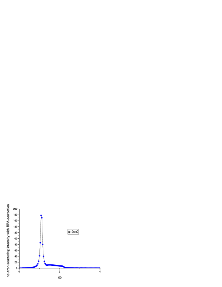
FIG. 11.: Neutron scattering intensity $I(\mathchoice{{\hbox{\boldmath$\displaystyle q$}}}{{\hbox{\boldmath$\textstyle q$}}}{{\hbox{\boldmath$\scriptstyle q$}}}{{\hbox{\boldmath$\scriptscriptstyle q$}}},\omega)$ at zero temperature vs. $\omega$ (in units of $\tilde{J}={3\over 8}J$) at $\mathchoice{{\hbox{\boldmath$\displaystyle q$}}}{{\hbox{\boldmath$\textstyle q$}}}{{\hbox{\boldmath$\scriptstyle q$}}}{{\hbox{\boldmath$\scriptscriptstyle q$}}}=(\pi,\pi)$.

Another probe which couples to the orbital current is Raman scattering. However, since the excitation is epected to peak at $(\pi,\pi)$, the large momentum transfer requires X-ray Raman scattering. It is known that X-ray couples to magnetic moments as well as orbital moments.[33] The moment due to the orbital current is weak and corresponds in strength to roughly $0.1\mu_{B}$. While Bragg scattering from an ordered spin moment has been observed,[34] inelastic scattering from a short-range order of such a small moment is beyond the current capability of X-ray scattering. We note, however, that polarization dependence is a powerful tood to distinguish between spin and orbital contributions in X-ray scattering.[33]

Next we discuss the possible measurement of the $\phi$ gauge modes. As discussed before, these modes involve the modulation of the amplitude of the hopping parameter $\chi_{ij}$ and the pairing parameter $\Delta_{ij}$ in a staggered fashion, i.e., with momentum $(\pi,\pi)$. The amplitude fluctuations of the superconducting order parameter is not easy to detect and has been experimentally observed only in the special case of superconductivity in a charge density wave system.[35, 36] On the other hand, the fluctuations in $\chi_{ij}$ couples to the quasiparticle hopping matrix element. In the mean field theory we can write an effective coupling as

$$H_{1}=-xt\sum_{<ij>\sigma}e^{i(e/c)A_{ij}}f_{i\sigma}^{\dagger}f_{j\sigma}+c.c.$$ (99)

where we include $A_{i,i+\mu}=aA_{\mu}$ as the lattice version of the electromagnetic field $\textstyle A$. Expansion of Eq.(66) to first order in $A_{ij}$ yields the standard $\mathchoice{{\hbox{\boldmath$\displaystyle j$}}}{{\hbox{\boldmath$\textstyle j$}}}{{\hbox{\boldmath$\scriptstyle j$}}}{{\hbox{\boldmath$\scriptscriptstyle j$}}}\cdot\mathchoice{{\hbox{\boldmath$\displaystyle A$}}}{{\hbox{\boldmath$\textstyle A$}}}{{\hbox{\boldmath$\scriptstyle A$}}}{{\hbox{\boldmath$\scriptscriptstyle A$}}}$ coupling. When expanded to second order we obtain ${1\over 2}xt\left({e\over c}\right)^{2}A_{ij}^{2}\left(f_{i\sigma}^{\dagger}f_{j\sigma}+c.c.\right)$. This gives rise to Raman scattering which is coupled to fluctuations in $\chi_{ij}$. This kind of coupling was discussed by Shastry and Shraiman[37] as an explanation of the continuum background due to incoherent electronic excitations. Here we expect that Raman scattering will couple to the transverse and longitudinal $\phi$ gauge mode. Physically, a modulation of $|\chi_{ij}|$ is a modulation of the bond charge density which should couple to Raman scattering. Standard Raman scattering provides essentially zero momentum transfer. In order to couple to the $\phi$ gauge mode at $(\pi,\pi)$ and to follow its dispersion, X-ray Raman scattering will be needed. The leading contribution to inelastic X-ray scattering originates from the ${e^{2}\over 2mc^{2}}\mathchoice{{\hbox{\boldmath$\displaystyle A$}}}{{\hbox{\boldmath$\textstyle A$}}}{{\hbox{\boldmath$\scriptstyle A$}}}{{\hbox{\boldmath$\scriptscriptstyle A$}}}^{2}$ term in the single particle Hamiltonian and the scattering cross-section is usually written as[38]

$${d^{2}\sigma\over d\Omega d\omega}=\left({d\sigma\over d\Omega}\right)_{Th}S(q,\omega)$$ (100)

where the Thomson cross-section is

$$\left({d\sigma\over d\Omega}\right)_{Th}=r_{0}^{2}\left(\hat{\epsilon}_{1}\cdot\hat{\epsilon}_{2}\right)^{2}{\omega_{2}\over\omega_{1}}\,\,\,,$$ (101)

$r_{0}=e^{2}/mc^{2}$ is the Thomson radius, $\hat{\epsilon}_{1},\omega_{1}$, and $\hat{\epsilon}_{2},\omega_{2}$ are the incident and scattering polarization vector and frequency, respectively, and $S(q,\omega)$ is the Fourier transform of the electron density-density correlation function. On a lattice, the corresponding matrix element comes from the second-order expansion of Eq.(66) and can be written as

$${1\over 2}\sum_{<i,j>}xt\left({e\over c}\right)^{2}A_{ij}^{2}\left(f_{i\sigma}^{\dagger}f_{j\sigma}+c.c.\right)$$ (102)

$$={x\over 4}\left({m\over m^{*}}\right)\left({e^{2}\over mc^{2}}\right){1\over 2}\sum_{i,\mu}\mathchoice{{\hbox{\boldmath$\displaystyle A$}}}{{\hbox{\boldmath$\textstyle A$}}}{{\hbox{\boldmath$\scriptstyle A$}}}{{\hbox{\boldmath$\scriptscriptstyle A$}}}^{2}_{\mu}(r_{i})\left(f_{i\sigma}^{\dagger}f_{i+\mu\sigma}+c.c.\right)$$ (103)

where the sum is over nearest neighbors and $ta^{2}={1\over 4m^{\ast}}$. Apart from ${m\over m^{\ast}}$, which is of order ${1\over 2}$, we see that the coupling is similar to the continuum theory, except that the number operator $f_{i\sigma}^{\dagger}f_{i\sigma}$ is replaced by ${1\over 4}\left(f_{i\sigma}^{\dagger}f_{i+\mu\sigma}+c.c.\right)$. Furthermore, a factor $x$ arises due to the strong correlation. We see from Eq.(69) that X-ray Raman scattering directly couples to the fluctuating in $\chi_{ij}$ and therefore to the $\phi$ gauge mode. It seems that high resolution inelastic X-ray scattering is a promising technique to observe the appearance of the $\phi$ gauge mode at low temperatures. The cross-section for X-ray scattering is proportional to $<|\gamma(\mathchoice{{\hbox{\boldmath$\displaystyle q$}}}{{\hbox{\boldmath$\textstyle q$}}}{{\hbox{\boldmath$\scriptstyle q$}}}{{\hbox{\boldmath$\scriptscriptstyle q$}}},\omega)|^{2}>$ where

$$\gamma(\mathchoice{{\hbox{\boldmath$\displaystyle q$}}}{{\hbox{\boldmath$\textstyle q$}}}{{\hbox{\boldmath$\scriptstyle q$}}}{{\hbox{\boldmath$\scriptscriptstyle q$}}},\omega)=\sum_{\mu}\hat{\epsilon}^{\prime}_{\mu}\hat{\chi}_{\mu}(\mathchoice{{\hbox{\boldmath$\displaystyle q$}}}{{\hbox{\boldmath$\textstyle q$}}}{{\hbox{\boldmath$\scriptstyle q$}}}{{\hbox{\boldmath$\scriptscriptstyle q$}}},\omega)\hat{\epsilon}_{\mu}\,\,\,,$$ (104)

$\hat{\epsilon}$ and $\hat{\epsilon}^{\prime}$ are the incoming and outgoing photon polarization and $\hat{\chi}_{\mu}(\mathchoice{{\hbox{\boldmath$\displaystyle q$}}}{{\hbox{\boldmath$\textstyle q$}}}{{\hbox{\boldmath$\scriptstyle q$}}}{{\hbox{\boldmath$\scriptscriptstyle q$}}},\omega)$ is the Fourier transform of the kinetic energy operator defined in Eq.(58). Thus the Raman scattering is given in terms of

$$S_{\mu\nu}^{\chi}(\mathchoice{{\hbox{\boldmath$\displaystyle q$}}}{{\hbox{\boldmath$\textstyle q$}}}{{\hbox{\boldmath$\scriptstyle q$}}}{{\hbox{\boldmath$\scriptscriptstyle q$}}},\omega)=<\hat{\chi}_{\mu}(\mathchoice{{\hbox{\boldmath$\displaystyle q$}}}{{\hbox{\boldmath$\textstyle q$}}}{{\hbox{\boldmath$\scriptstyle q$}}}{{\hbox{\boldmath$\scriptscriptstyle q$}}},\omega)\hat{\chi}_{\nu}(\mathchoice{{\hbox{\boldmath$\displaystyle q$}}}{{\hbox{\boldmath$\textstyle q$}}}{{\hbox{\boldmath$\scriptstyle q$}}}{{\hbox{\boldmath$\scriptscriptstyle q$}}},\omega)>\,\,\,.$$ (105)

This is computed numerically using the same method described by Eqs.(64) and (65). The results are shown in Fig. 12 along $(q_{x},\pi)$.

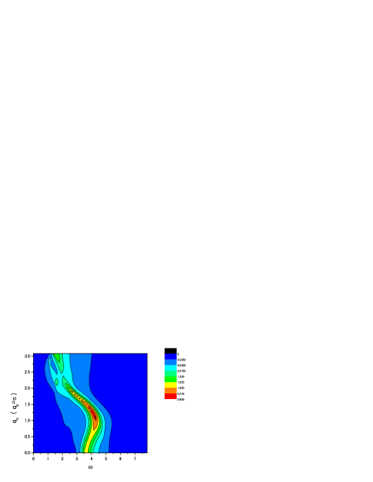
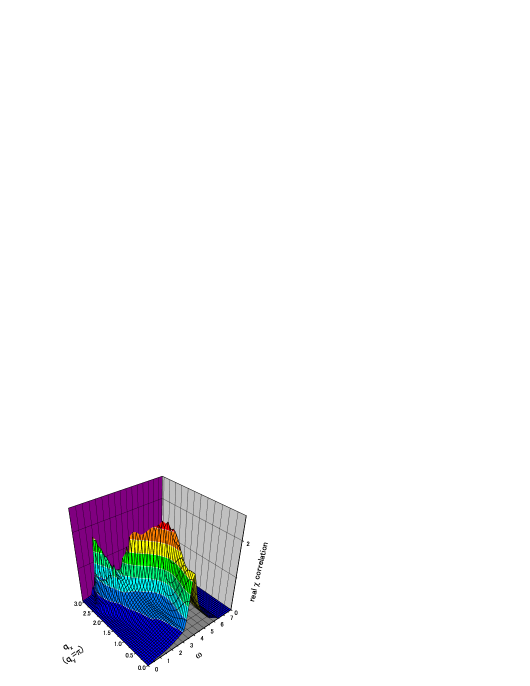
FIG. 12.: Spectral function $S_{\mu\mu}^{\chi}(\mathchoice{{\hbox{\boldmath$\displaystyle q$}}}{{\hbox{\boldmath$\textstyle q$}}}{{\hbox{\boldmath$\scriptstyle q$}}}{{\hbox{\boldmath$\scriptscriptstyle q$}}},\omega)(\mu=\hat{x})$ for the correlation of the kinetic energy operator [Eq.(71)] which is measured by inelastic X-ray scattering. A contour plot and a bird’s eye view are shown. $\textstyle q$ ranges from $(0,\pi)$ to $(\pi,\pi)$, i.e., $\mathchoice{{\hbox{\boldmath$\displaystyle q$}}}{{\hbox{\boldmath$\textstyle q$}}}{{\hbox{\boldmath$\scriptstyle q$}}}{{\hbox{\boldmath$\scriptscriptstyle q$}}}=(q_{x},\pi)$. Frequency $\omega$ is in units of $\tilde{J}(={3\over 8}J)$.

The spectral function is peaked at $(\pi,\pi)$ as expected. Note that along the $(\mathchoice{{\hbox{\boldmath$\displaystyle q$}}}{{\hbox{\boldmath$\textstyle q$}}}{{\hbox{\boldmath$\scriptstyle q$}}}{{\hbox{\boldmath$\scriptscriptstyle q$}}}_{x},\pi)$ direction (Fig.12) the spectral function has similar structure as the longitudinal $\phi$ gauge mode (Fig.8).

The spectral function at $\mathchoice{{\hbox{\boldmath$\displaystyle q$}}}{{\hbox{\boldmath$\textstyle q$}}}{{\hbox{\boldmath$\scriptstyle q$}}}{{\hbox{\boldmath$\scriptscriptstyle q$}}}=(\pi,\pi)$ is shown in Fig.13. We note that its shape is quite similar to that of the amplitude mode shown in Fig.10. For completeness, we also computed the correlation $S_{\Delta}=<\delta\Delta_{\mu}\delta\Delta_{\mu}>$ where $\Delta_{\mu}$ was defined in Eq.(59). This describes the fluctuations of the real part of $\Delta_{ij}$ and would correspond to the conventional superconducting amplitude mode. As shown in Fig.14, its shape is similar to that of the $\phi$ gauge mode.

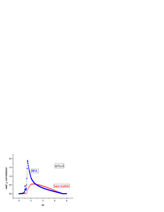
FIG. 13.: The lineshape of the kinetic operator correlator $S^{\chi}_{\mu,\mu}(\mathchoice{{\hbox{\boldmath$\displaystyle q$}}}{{\hbox{\boldmath$\textstyle q$}}}{{\hbox{\boldmath$\scriptstyle q$}}}{{\hbox{\boldmath$\scriptscriptstyle q$}}},\omega)$ $(\mu=\hat{x})$ as a function of $\omega$ (in units of $\tilde{J}={3\over 8}J$) at $\mathchoice{{\hbox{\boldmath$\displaystyle q$}}}{{\hbox{\boldmath$\textstyle q$}}}{{\hbox{\boldmath$\scriptstyle q$}}}{{\hbox{\boldmath$\scriptscriptstyle q$}}}=(\pi,\pi)$. This is the curve labeled as RPA. Also shown is the curve labeled as bare bubble, which is computed by coupling to particle-hole excitations without allowing any collective enhancement.

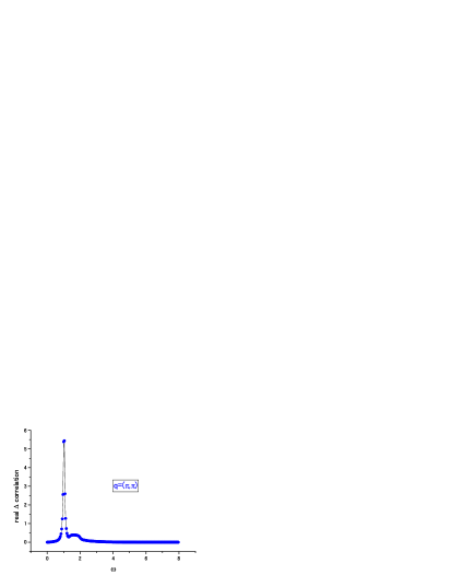
FIG. 14.: The spectral function $S_{\Delta}(\mathchoice{{\hbox{\boldmath$\displaystyle q$}}}{{\hbox{\boldmath$\textstyle q$}}}{{\hbox{\boldmath$\scriptstyle q$}}}{{\hbox{\boldmath$\scriptscriptstyle q$}}},\omega)$ at $\mathchoice{{\hbox{\boldmath$\displaystyle q$}}}{{\hbox{\boldmath$\textstyle q$}}}{{\hbox{\boldmath$\scriptstyle q$}}}{{\hbox{\boldmath$\scriptscriptstyle q$}}}=(\pi,\pi)$.

Given that $\delta\chi$ and $\delta\Delta$ are linear superpositions of $\delta A$ and $\delta\phi$ according to Eqs.(56,60), it is surprising that their spectral functions are not simply weighted averages of the amplitude and $\phi$ gauge modes. The reason is that there is significant cross-correlation between $\delta\chi$ and $\delta\Delta$, as well as between $\delta A$ and $\delta\phi$, i.e., the amplitude and $\phi$ fluctuations are not truly eigenmodes. This is a consequence of the significant mixing at $x=0.1$ between these modes at finite frequencies as discussed earlier. It is perhaps better to focus on $S^{\chi}_{\mu,\nu}$ which is experimentally measurable. The peak observed in $S^{\chi}_{\mu,\mu}$ corresponds to collective oscillations of the hopping matrix element. This is a new degree of freedom not present in conventional superconductors. To emphasize this point we have also computed the “bare bubble” response, i.e., using $M^{F}_{\alpha\beta}$ without the collective enhancement shown in in Eq.(65). As seen in Fig.13, the latter is much more spread out in frequency. Finally we note that for the relatively high doping considered here, the $\phi$ gauge mode appears to be closely related to the more conventional superconductor amplitude fluctuation $\delta\Delta_{\mu}$ (albeit at $\mathchoice{{\hbox{\boldmath$\displaystyle q$}}}{{\hbox{\boldmath$\textstyle q$}}}{{\hbox{\boldmath$\scriptstyle q$}}}{{\hbox{\boldmath$\scriptscriptstyle q$}}}=(\pi,\pi)$) and is difficult to detect.

We note that since $\chi_{ij}$ couples to the quasiparticle hopping matrix element, it in turn is coupled to phonons. In Appendix B we consider the possibility that the collective modes may appear as phonon sidebands which may be detected optically.

VII Conclusion

We have shown that in the gauge theory description of the $t$-$J$ model, new collective modes appear in the superconducting ground state. The SU(2) gauge theory allows us to classify these collective modes and predict them analytically. These predictions are confirmed by numerical computation of the collective mode spectra. In particular, we see that the SU(2) formulation allows us to smoothly connect to the $x=0$ limit, whereas in the U(1) formulation, spurious modes would have appeared.

In this paper we describe the bosons in the radial gauge. It is then clear that boson dynamics do not play a role and that collective modes dynamics are entirely determined by the fermions via the fermion bubbles which make up the matrix $M^{F}$. In Ref. (24) we proposed a $\sigma$-model formulation where the low-lying excitations are parametrized by the boson $h=\sqrt{x}z=\sqrt{x}\pmatrix{z_{1}\cr z_{2}}$. We proposed an effective action which included a term $xz^{\dagger}D_{0}z$ where $D_{0}=\partial_{\tau}+eA_{0}+a_{0}^{3}\tau^{3}$ [Eq.(78) Ref. (24)]. Note that this term produces a coupling between the $\theta$ and $\phi$ modes of the form $\delta\theta\partial_{\tau}\phi$. This Berry’s phase term is absent in the present paper. Thus Eq.(78) of ref. (24) disagrees with the present work and we believe that it is incorrect. Within the $\sigma$-model approach in ref. (24), one should have absorbed the $z^{\dagger}\partial_{\tau}z$ term into the $z^{\dagger}a_{0}^{3}\tau^{3}z$ term by a gauge transformation and solve for the $a_{0}^{\prime\ell}$ terms by imposing the constraint locally. That is in fact what is done in this paper for small $\delta\theta$ and $\delta\phi$. A similar procedure can be adopted for arbitrary $\theta$ and $\phi$ to generate a $\sigma$-model. Thus the $\sigma$-model should be viewed as a way to parametrize the low-lying fluctuation of the $U_{ij}$ matrix [as in Eq.(40)] and the effective action depends only on the fermion dynamics.

The appearance of the new collective modes answers the question of whether the superconducting state described by the gauge theory is any different from a conventional BCS state. The $\theta$ mode is coupled to staggered orbital currents. The importance of these currents was already revealed in the Gutzwiller projected BCS wavefunction.[17] In principle, they should be observable by neutron scattering or X-ray Raman scattering. A new collective degree of freedom is the moduation of the hopping amplitude which is observable by high resolution inelastic X-ray scattering. We also show how they give rise to side-bands in certain phonon modes. However, the weakness of the coupling makes its observation difficult. The predictions of these collective modes are unique features of the slave-boson/gauge-field approach to the $t$-$J$ model and experimental searches for the collective modes will serve as important tests of this line of approach to the high T_c problem.

A Derivation of the effective action for collective modes

In this appendix, we sketch the calculation of the effective action for the collective modes up to quadratic order. For simplicity, we consider here the case of $t^{\prime}=0$. The inclusion of $t^{\prime}$-term is rather trivial. We start with the Lagrangian Eq.(21) in the text, because we consider the superconducting ground state with the bose condensation. The procedure is standard as in the usual 1/N expansion. Namely we first divide the integral variables into the mean field (saddle point) values and the fluctuations as given in Eq.(24). Integrating over the fermionic integral variables, we can expand the effective action with respect to the fluctuating part $\delta U_{ij}$, $\delta a_{0}^{3}$, $\delta a_{0}^{1},\delta a_{0}^{2}$, and $\delta R$.

Then the stationary condition that the linear order terms in $\delta U_{ij}$ etc. vanish gives the self-consistent mean field equations as

$$\chi=\int_{-\pi}^{\pi}{{dk_{x}}\over{2\pi}}\int_{-\pi}^{\pi}{{dk_{y}}\over{2\pi}}{{-\xi_{k}\gamma_{k}}\over{2E_{k}}}=\int{d^{2}\mathchoice{{\hbox{\boldmath$\displaystyle k$}}}{{\hbox{\boldmath$\textstyle k$}}}{{\hbox{\boldmath$\scriptstyle k$}}}{{\hbox{\boldmath$\scriptscriptstyle k$}}}\over(2\pi)^{2}}{{-\xi_{k}\gamma_{k}}\over{2E_{k}}}$$ (A1)

$$\Delta=\int{d^{2}\mathchoice{{\hbox{\boldmath$\displaystyle k$}}}{{\hbox{\boldmath$\textstyle k$}}}{{\hbox{\boldmath$\scriptstyle k$}}}{{\hbox{\boldmath$\scriptscriptstyle k$}}}\over(2\pi)^{2}}{{{\tilde{J}}\Delta\beta_{k}^{2}}\over{E_{k}}}$$ (A2)

$$\lambda_{0}=\int{d^{2}\mathchoice{{\hbox{\boldmath$\displaystyle k$}}}{{\hbox{\boldmath$\textstyle k$}}}{{\hbox{\boldmath$\scriptstyle k$}}}{{\hbox{\boldmath$\scriptscriptstyle k$}}}\over(2\pi)^{2}}{{2{\tilde{t}}\gamma_{k}\xi_{k}}\over{E_{k}}}$$ (A3)

where $\gamma_{k}=\cos k_{x}+\cos k_{y}$, $\beta_{k}=\cos k_{x}-\cos k_{y}$, and $E_{k}=\sqrt{\xi_{k}^{2}+\Delta_{k}^{2}}$ with $\xi_{k}$ and $\Delta_{k}$ being given below eq.(23).

The Gaussian fluctuations are represented by the quadratic terms $S_{2}$.

$$S_{2} = \int_{0}^{\beta}d\tau\biggl{[}{\tilde{J}}\sum_{i,\mu=x,y}\bigl{(}|\delta\chi_{ii+\mu}|^{2}+|\delta\Delta_{ii+\mu}|^{2}\bigr{)}-r_{0}^{2}\sum_{i}\bigl{(}2i\delta a^{3}_{0}(i)\delta R_{i}+\lambda_{0}(\delta R_{i})^{2}\bigr{)}$$ (A4)

$$- \sum_{<i,j>\sigma}r_{0}^{2}{\tilde{t}}_{ij}\delta R_{i}\delta R_{j}<f^{\dagger}_{i\sigma}f_{j\sigma}+f^{\dagger}_{j\sigma}f_{i\sigma}>\biggr{]}$$ (A5)

$$+ {1\over 2}Tr[GVGV]$$ (A6)

where $\beta$ is the inverse temperature and the last term represents the second order contributions from the fermionic determinant. Here the Green’s function is $2\times 2$ matrix for each $k=({\mathchoice{{\hbox{\boldmath$\displaystyle k$}}}{{\hbox{\boldmath$\textstyle k$}}}{{\hbox{\boldmath$\scriptstyle k$}}}{{\hbox{\boldmath$\scriptscriptstyle k$}}}},\omega_{n})$ ($\textstyle k$: wave vector, $\omega_{n}$: fermionic Matsubara frequency). Then the explicit form of the last term in eq.(A4) is ($q=({\mathchoice{{\hbox{\boldmath$\displaystyle q$}}}{{\hbox{\boldmath$\textstyle q$}}}{{\hbox{\boldmath$\scriptstyle q$}}}{{\hbox{\boldmath$\scriptscriptstyle q$}}}},\omega_{m})$)

$${1\over{2\beta V}}\sum_{q}\sum_{k}tr[G(k-q/2)V(k-q/2,k+q/2)G(k+q/2)V(k+q/2,k-q/2)],$$ (A7)

where $tr$ means the trace over the $2\times 2$ matrix. The Green’s function is given by,

$$[G(k)]^{-1}=\pmatrix{i\omega_{n}-\xi_{\mathchoice{{\hbox{\boldmath$\displaystyle k$}}}{{\hbox{\boldmath$\textstyle k$}}}{{\hbox{\boldmath$\scriptstyle k$}}}{{\hbox{\boldmath$\scriptscriptstyle k$}}}}&,&-\Delta_{\mathchoice{{\hbox{\boldmath$\displaystyle k$}}}{{\hbox{\boldmath$\textstyle k$}}}{{\hbox{\boldmath$\scriptstyle k$}}}{{\hbox{\boldmath$\scriptscriptstyle k$}}}}\cr-\Delta_{k}&,&i\omega_{n}+\xi_{\mathchoice{{\hbox{\boldmath$\displaystyle k$}}}{{\hbox{\boldmath$\textstyle k$}}}{{\hbox{\boldmath$\scriptstyle k$}}}{{\hbox{\boldmath$\scriptscriptstyle k$}}}}},$$ (A8)

which is represented in a compact form in terms of the Pauli matrices $\tau^{1},\tau^{2},\tau^{3}$ as

$$G(k)=-[\omega_{n}^{2}+E_{k}^{2}]^{-1}[i\omega_{n}+\Delta_{k}\tau^{1}-\xi_{k}\tau^{3}].$$ (A9)

The matrix $V$ is explicitely given by

$$V(k+q/2,k-q/2)={{2{\tilde{J}}}\over{\sqrt{\beta V}}}\sum_{\mu=x,y}$$ (A10)

$$\times \pmatrix{-i\delta a_{0}^{3}(q)-\delta\chi^{\prime\prime}_{\mu}(q)\sin k_{\mu}-\delta\chi^{\prime}_{\mu}(q)\cos k_{\mu}&,&-i\delta a_{0}^{1}(q)-\delta a_{0}^{2}(q)+\delta\Delta^{\prime}_{\mu}(q)\cos k_{\mu}+i\delta\Delta^{\prime\prime}_{\mu}(q)\cos k_{\mu}\cr-i\delta a_{0}^{1}(q)+\delta a_{0}^{2}(q)+\delta\Delta^{\prime}_{\mu}(q)\cos k_{\mu}-i\delta\Delta^{\prime\prime}_{\mu}(q)\cos k_{\mu}&,&+i\delta a_{0}^{3}(q)-\delta\chi^{\prime\prime}_{\mu}(q)\sin k_{\mu}+\delta\chi^{\prime}_{\mu}(q)\cos k_{\mu}}.$$ (A11)

Here it is noted that $\delta U_{ij}$ is represented as

$$\delta U_{ii+\mu}=-\delta\chi^{\prime}_{\mu}(i)\tau^{3}+i\delta\chi^{\prime\prime}_{\mu}(i)+\delta\Delta^{\prime}_{\mu}(i)\tau^{1}-\delta\Delta^{\prime\prime}_{\mu}(i)\tau^{2}$$ (A12)

where $\chi_{\mu}(i)=\chi^{\prime}_{\mu}(i)+i\chi^{\prime\prime}_{\mu}(i)$, and $\Delta_{\mu}(i)=\Delta^{\prime}_{\mu}(i)+i\Delta^{\prime\prime}_{\mu}(i)$. The Fourier transformations of these variables are defined as

$$\chi^{\prime}_{\mu}(i,\tau)={1\over{\sqrt{\beta V}}}\sum_{q}\chi^{\prime}_{\mu}(q)e^{-i\omega_{m}\tau+i{\mathchoice{{\hbox{\boldmath$\displaystyle q$}}}{{\hbox{\boldmath$\textstyle q$}}}{{\hbox{\boldmath$\scriptstyle q$}}}{{\hbox{\boldmath$\scriptscriptstyle q$}}}}\cdot{\mathchoice{{\hbox{\boldmath$\displaystyle R$}}}{{\hbox{\boldmath$\textstyle R$}}}{{\hbox{\boldmath$\scriptstyle R$}}}{{\hbox{\boldmath$\scriptscriptstyle R$}}}}_{i+\mu/2}},$$ (A13)

and similar expressions for other variables. We define the 12 variables $X_{\alpha}(q)$ ($\alpha=1,...,12$) as

$$X(q)=\pmatrix{\delta\chi^{\prime\prime}_{x}(q)\cr\delta\chi^{\prime\prime}_{y}(q)\cr\delta\Delta^{\prime}_{x}(q)\cr\delta\Delta^{\prime}_{y}(q)\cr\delta\Delta^{\prime\prime}_{x}(q)\cr\delta\Delta^{\prime\prime}_{y}(q)\cr\delta\chi^{\prime}_{x}(q)\cr\delta\chi^{\prime}_{y}(q)\cr\delta R(q)\cr\delta a^{1}_{0}(q)\cr\delta a^{2}_{0}(q)\cr\delta a^{3}_{0}(q)}$$ (A14)

In the calculation of the fermionic polarization function the following integrals are needed.

$$F_{ab}({\mathchoice{{\hbox{\boldmath$\displaystyle q$}}}{{\hbox{\boldmath$\textstyle q$}}}{{\hbox{\boldmath$\scriptstyle q$}}}{{\hbox{\boldmath$\scriptscriptstyle q$}}}},\omega_{m};{\mathchoice{{\hbox{\boldmath$\displaystyle k$}}}{{\hbox{\boldmath$\textstyle k$}}}{{\hbox{\boldmath$\scriptstyle k$}}}{{\hbox{\boldmath$\scriptscriptstyle k$}}}})={1\over{\beta}}\sum_{\omega_{n}}tr[G(k+q/2)\tau^{a}G(k-q/2)\tau^{b}],$$ (A15)

where $\tau^{0}=1$ (unit matrix) and $\tau^{1,2,3}$ are Pauli matrices. At zero temperature, the summation over $\omega_{n}$ is reduced to the integral, i.e., $\beta^{-1}\sum_{\omega_{n}}\to\int d\omega/2\pi$, which can be done to result in the following $4\times 4$ matrix.

$$F({\mathchoice{{\hbox{\boldmath$\displaystyle q$}}}{{\hbox{\boldmath$\textstyle q$}}}{{\hbox{\boldmath$\scriptstyle q$}}}{{\hbox{\boldmath$\scriptscriptstyle q$}}}},\omega_{m})=$$ (A16)

$$\left(\matrix{(\omega_{m}^{2}/4+\chi_{+}\chi_{-}+\Delta_{+}\Delta_{-})I_{1}-I_{3},&i(\Delta_{+}+\Delta_{-})I_{2}+i\omega_{m}(\Delta_{-}-\Delta_{+})I_{1}/2,\cr i(\Delta_{+}+\Delta_{-})I_{2}+i\omega_{m}(\Delta_{-}-\Delta_{+})I_{1}/2,&(\omega_{m}^{2}/4-\chi_{+}\chi_{-}+\Delta_{+}\Delta_{-})I_{1}-I_{3},\cr i(\chi_{+}\Delta_{-}-\chi_{-}\Delta_{+})I_{1},&(-\chi_{+}+\chi_{-})I_{2}+\omega_{m}(\chi_{+}+\chi_{-})I_{1}/2,\cr-i(\chi_{+}+\chi_{-})I_{2}+i\omega_{m}(\chi_{+}-\chi_{-})I_{1}/2,&-(\chi_{+}\Delta_{-}+\chi_{-}\Delta_{+})I_{1},\cr}\right.$$ (A17)

$$\rule{137.31255pt}{0.0pt}\left.\matrix{i(-\chi_{+}\Delta_{-}+\chi_{-}\Delta_{+})I_{1},&-i(\chi_{+}+\chi_{-})I_{2}+i\omega_{m}(\chi_{+}-\chi_{-})I_{1}/2\cr(\chi_{+}-\chi_{-})I_{2}-\omega_{m}(\chi_{+}+\chi_{-})I_{1}/2,&-(\chi_{+}\Delta_{-}+\chi_{-}\Delta_{+})I_{1}\cr(\omega_{m}^{2}/4-\chi_{+}\chi_{-}-\Delta_{+}\Delta_{-})I_{1}-I_{3},&(-\Delta_{+}+\Delta_{-})I_{2}+\omega_{m}(\Delta_{+}+\Delta_{-})I_{1}/2\cr(\Delta_{+}-\Delta_{-})I_{2}-\omega_{m}(\Delta_{+}+\Delta_{-})I_{1}/2,&(\omega_{m}^{2}/4+\chi_{+}\chi_{-}-\Delta_{+}\Delta_{-})I_{1}-I_{3}}\right)$$ (A18)

where

$$I_{1}(q) = {1\over{\omega_{m}^{4}+2\omega_{m}^{2}(E_{+}^{2}+E_{-}^{2})+(E_{+}^{2}-E_{-}^{2})^{2}}}\biggl{[}{{\omega_{m}^{2}-E_{+}^{2}+E_{-}^{2}}\over{2E_{+}}}+{{\omega_{m}^{2}+E_{+}^{2}-E_{-}^{2}}\over{2E_{-}}}\biggr{]}$$ (A19)

$$I_{2}(q) = {1\over{\omega_{m}^{4}+2\omega_{m}^{2}(E_{+}^{2}+E_{-}^{2})+(E_{+}^{2}-E_{-}^{2})^{2}}}\biggl{[}{{\omega_{m}(E_{+}-E_{-})[\omega_{m}^{2}+(E_{+}-E_{-})^{2}]}\over{4E_{+}E_{-}}}$$ (A20)

$$I_{3}(q) = {1\over{\omega_{m}^{4}+2\omega_{m}^{2}(E_{+}^{2}+E_{-}^{2})+(E_{+}^{2}-E_{-}^{2})^{2}}}\biggl{[}{{(E_{+}+E_{-})\omega_{m}^{4}}\over{8E_{+}E_{-}}}+{{(E_{+}+E_{-})^{3}\omega_{m}^{2}}\over{8E_{+}E_{-}}}+{{(E_{+}-E_{-})^{2}(E_{+}+E_{-})}\over{2}}\biggr{]}$$ (A21)

The static limit of these funcitons are easily estimated as

$$I_{1}({\mathchoice{{\hbox{\boldmath$\displaystyle q$}}}{{\hbox{\boldmath$\textstyle q$}}}{{\hbox{\boldmath$\scriptstyle q$}}}{{\hbox{\boldmath$\scriptscriptstyle q$}}}},\omega_{m}=0) = {1\over{2E_{+}E_{-}(E_{+}+E_{-})}}$$ (A22)

$$I_{2}({\mathchoice{{\hbox{\boldmath$\displaystyle q$}}}{{\hbox{\boldmath$\textstyle q$}}}{{\hbox{\boldmath$\scriptstyle q$}}}{{\hbox{\boldmath$\scriptscriptstyle q$}}}},\omega_{m}=0) = 0$$ (A23)

$$I_{3}({\mathchoice{{\hbox{\boldmath$\displaystyle q$}}}{{\hbox{\boldmath$\textstyle q$}}}{{\hbox{\boldmath$\scriptstyle q$}}}{{\hbox{\boldmath$\scriptscriptstyle q$}}}},\omega_{m}=0) = {1\over{2(E_{+}+E_{-})}}.$$ (A24)

Here we have introduced the abbrebiations such as $E_{\pm}=E_{{\mathchoice{{\hbox{\boldmath$\displaystyle k$}}}{{\hbox{\boldmath$\textstyle k$}}}{{\hbox{\boldmath$\scriptstyle k$}}}{{\hbox{\boldmath$\scriptscriptstyle k$}}}}\pm{\mathchoice{{\hbox{\boldmath$\displaystyle q$}}}{{\hbox{\boldmath$\textstyle q$}}}{{\hbox{\boldmath$\scriptstyle q$}}}{{\hbox{\boldmath$\scriptscriptstyle q$}}}}/2}$ etc. Then the quadratic action $S_{2}$ with respect to the variables $X_{\alpha}$ is given by

$$S_{2} = \sum_{q}\biggl{[}\sum_{\alpha,\beta=1,12}\Pi_{\alpha\beta}(q)X_{\alpha}(q)X_{\beta}(-q)$$ (A25)

$$+ \sum_{\alpha=1,8}{\tilde{J}}X_{\alpha}(q)X_{\alpha}(-q)-ix(X_{12}(q)X_{9}(-q)+X_{12}(q)X_{9}(-q))-{{x\lambda_{0}}\over 2}(\cos q_{x}+\cos q_{y})X_{9}(q)X_{9}(-q).\biggr{]}$$ (A26)

Here

$$\Pi_{\alpha\beta}={1\over V}\sum_{k}\zeta_{\alpha}(k)\zeta_{\beta}(k)F_{a(\alpha),a(\beta)}({\mathchoice{{\hbox{\boldmath$\displaystyle q$}}}{{\hbox{\boldmath$\textstyle q$}}}{{\hbox{\boldmath$\scriptstyle q$}}}{{\hbox{\boldmath$\scriptscriptstyle q$}}}},\omega_{m};{\mathchoice{{\hbox{\boldmath$\displaystyle k$}}}{{\hbox{\boldmath$\textstyle k$}}}{{\hbox{\boldmath$\scriptstyle k$}}}{{\hbox{\boldmath$\scriptscriptstyle k$}}}})$$ (A27)

where

$$\zeta(k)=\pmatrix{-2\sin k_{x}\cr-2\sin k_{y}\cr 2\cos k_{x}\cr 2\cos k_{y}\cr-2\cos k_{x}\cr-2\cos k_{y}\cr-2\cos k_{x}\cr-2\cos k_{y}\cr-4x{\tilde{t}}(\cos(k_{x})\cos(q_{x}/2)+\cos(k_{y})\cos(q_{y}/2))\cr-1\cr-1\cr-1}$$ (A28)

and $a(\alpha)$ is the index of the Pauli matrix corresponding to each component and is given as $a(1)=a(2)=0,a(3)=a(4)=1,a(5)=a(6)=2,a(7)=a(8)=a(9)=3,a(10)=1,a(11)=2,a(12)=3$. The fermion bubble is analytically continued in the standard way as $F(i\omega_{m}\rightarrow\omega+i\eta)$. Equation (A16) is numerically evaluated by discretizing the 1st Brillouin zone by $200\times 200$ and treating $\eta$ as small but finite. The convergence with respect to the number of the lattice points has been checked.

Equation (A15) is the quadatic forms for the 12 variables $X_{\alpha}$, and by integrating over the last 3 variables $X_{10},X_{11},X_{12}(=\delta a_{0}^{1},\delta a_{0}^{2},\delta a_{0}^{3})$, we obtain the effective action for 9 variables, which has positive definite engenvalues for each $q=({\mathchoice{{\hbox{\boldmath$\displaystyle q$}}}{{\hbox{\boldmath$\textstyle q$}}}{{\hbox{\boldmath$\scriptstyle q$}}}{{\hbox{\boldmath$\scriptscriptstyle q$}}}},\omega_{m})$ when the mean field solution is stable.

B Coupling of the $\phi$ Gauge Mode to Phonons

Let us consider the mode where the planar oxygen moves in and out of the plane. We focus on the oxygen mode because the mass is light and the frequency relatively low, and both features tend to enhance the coupling. In LSCO and YBCO, the oxygen is buckled out of the plane. (In YBCO the displacement $u_{0}=0.256$ Angstroms.) Then the out-of-plane phonon mode has a linear coupling to the Cu-O bond length and therefore to the effective hopping $t$ and exchange $J$. This problem was considered by Normand et al.[39] who concluded that in YBCO

$$\delta t_{ij} = \lambda_{t}t\delta u_{ij}/a$$ (B1)

$$\delta J_{ij} = \lambda_{J}J\delta u_{ij}/a$$ (B2)

where they estimate $\lambda_{t}\approx{1\over 2}\lambda_{J}\approx 2.6$ for a displacement $\delta u_{ij}$ of the oxygen on the $ij$ bond normal to the plane. The surprising large coupling is partly due to the fact that the displacement $\delta u_{ij}$ is normalized to the lattice constant $a\approx 4$ Angstroms which is quite large. Let us first focus on the $\delta t_{ij}$ term. The modulation of the Hamiltonian is

$$\delta H_{t} = \sum_{<ij>\sigma}\delta t_{ij}c_{i\sigma}^{\dagger}c_{j\sigma}$$ (B3)

$$\approx \sum_{<ij>,\sigma}\lambda_{t}t{\delta u_{ij}\over a}b_{i}b_{j}^{\dagger}f_{i\sigma}f_{j\sigma}^{\dagger}$$ (B4)

$$\approx \lambda_{t}(\chi_{0}+\delta\chi_{ij})xt{\delta u_{ij}\over a}$$ (B5)

The last line is in the mean field approximation, where we retained the amplitude fluctuation $\delta\chi_{ij}$ of $\chi_{ij}$.

Next, recall that the $\phi$ gauge mode couples to $\chi_{ij}$ via Eqs.(37) and (38), so that

$$\delta\chi_{ij}=-\Delta_{0}(-1)^{i_{x}+i_{y}}v_{ij}\,\,\,.$$ (B6)

Combining Eqs.(B3) and (B4), we find an effective coupling between the pnonon displacement and the $\phi$ guage mode co-ordinate

$$H_{eff} = -\lambda_{eff}(-1)^{i_{x}+i_{y}}{\delta u_{ij}\over a}v_{ij}$$ (B7)

where

$$\lambda_{eff}=\lambda_{t}xt\Delta_{0}\,\,\,.$$ (B8)

Note that a fluctuation of $v_{ij}$ couples to a $(\pi,\pi)$ phonon mode as expected. It turns out that the modulation of $J$ given by Eq.(B2) does not couple to the $\phi$ gauge mode. The reason is that in mean field, the modulation of the $J$ term is $\delta J_{ij}(\chi_{ij}^{\ast}\chi_{ij}+\Delta_{ij}^{\ast}\Delta_{ij})$. This couples to the amplitude mode. On the other hand, in the $\phi$ gauge mode, the total modulus $|\chi_{ij}|^{2}+|\Delta_{ij}|^{2}$ is held fixed, as shown in Fig. 2. Thus there is no coupling between the $\phi$ gauge mode and the phonon via the $\delta J_{ij}$ term.

We next approximate the phonon as an Einstein model. The energy is given by ${1\over 2}(-\omega^{2}+\omega_{0}^{2})a^{2}M\left({\delta u\over a}\right)^{2}$ where $\omega_{0}$ is the frequency and $M$ is the mass. We approximate the gauge mode as a well defined mode at frequency $\omega_{\phi}$ with energy ${1\over 2}{\alpha_{\phi}\over\omega_{\phi}}(-\omega^{2}+\omega_{\phi}^{2})v_{ij}^{2}$ and adjust $\alpha_{\phi}$ to match the spectral weight. The coupled phonon-$\phi$ gauge modes are obtained by diagonalizing the $2\times 2$ matrix

$$D^{-1}=\pmatrix{{1\over 2}{\alpha_{\phi}\over\omega_{\phi}}(-\omega^{2}+\omega_{\phi}^{2})&-\lambda_{eff}\cr-\lambda_{eff}&{1\over 2}(-\omega^{2}+\omega_{0}^{2})a^{2}M}\,\,\,.$$ (B9)

The modes are

$$\omega_{\pm}^{2}={1\over 2}\left[(\omega_{0}^{2}+\omega_{\phi}^{2})\pm\sqrt{(\omega_{0}^{2}-\omega_{\phi}^{2})^{2}+4g^{2}\omega_{0}^{4}}\,\,\right]$$ (B10)

where the dimensionless coupling constant is

$$g^{2}={4\lambda_{eff}^{2}\omega_{\phi}\over a^{2}M\omega_{0}^{4}\alpha_{\phi}}$$ (B11)

The phonon Green’s function $D=\langle\delta u_{ij}\delta u_{ij}\rangle$ is

$$D={(-\omega^{2}+\omega_{\phi}^{2})\over(-\omega^{2}+\omega_{+}^{2})(-\omega^{2}+\omega_{-}^{2})a^{2}M}\,\,\,.$$ (B12)

Assuming $\omega_{0}>\omega_{\phi}$, the phonon mode is shifted slightly upwards in frequency to $\omega_{+}$ but a side band appears at $\omega_{-}$ which is near $\omega_{\phi}$. The ratio of the spectral weight of the $\omega_{-}$ side band to the $\omega_{+}$ mode is

$$R={\omega_{\phi}^{2}-\omega_{-}^{2}\over\omega_{+}^{2}-\omega_{\phi}^{2}}{\omega_{+}\over\omega_{-}}\,\,\,.$$ (B13)

For weak coupling $g^{2}<<1$, we expand the numerator using Eq.(B8) and replace $\omega_{+}$ by $\omega_{0}$ and $\omega_{-}$ by $\omega_{\phi}$ to obtain

$$R={g^{2}\omega_{0}^{4}\over\left(\omega_{0}^{2}-\omega_{\phi}^{2}\right)^{2}}\left({\omega_{0}\over\omega_{\phi}}\right)\,\,\,.$$ (B14)

This result for the relative spectral weight is also valid if $\omega_{0}<\omega_{\phi}$.

The spectral weight ratio is mainly determined by the coupling constant $g^{2}$. To make a rough estimate, we take $M=\mbox{\rm oxygen mass}\,\,\omega_{0}\approx J/4$ so that $a^{2}M\omega_{0}^{2}\approx 25\,\mbox{\rm eV}\approx 200J$. Taking $\lambda_{eff}\approx J/4$, we find

$$g^{2}\approx{1\over 200}{\omega_{\phi}\over\omega_{0}\alpha_{\phi}}\,\,\,.$$ (B15)

We estimate $\alpha_{\phi}\approx 1$ because we can see from Fig. 9 that the spectral weight of the $\phi$ gauge mode at $(\pi,\pi)$, is of order unity. Unfortunately, $g^{2}$ turns out to be very small.

The small spectral weight ($\sim 5\times 10^{-3}$ of the main phonon peak) means that it is probably impossible to observe the side-band by neutron scattering. Optical measurements offer higher precision. For YBCO the phonon is at $\mathchoice{{\hbox{\boldmath$\displaystyle q$}}}{{\hbox{\boldmath$\textstyle q$}}}{{\hbox{\boldmath$\scriptstyle q$}}}{{\hbox{\boldmath$\scriptscriptstyle q$}}}=(\pi,\pi)$ and do not couple to light. LSCO offers a special opportunity in that at low temperatures, the lattice is in the low temperature orthorhombic phase (LTO) where the buckeling of the oxygen is staggered, i.e., $u_{ij}=u_{0}(-1)^{i_{x}+i_{y}}$. Then a $\mathchoice{{\hbox{\boldmath$\displaystyle q$}}}{{\hbox{\boldmath$\textstyle q$}}}{{\hbox{\boldmath$\scriptstyle q$}}}{{\hbox{\boldmath$\scriptscriptstyle q$}}}=0$ distortion $u_{ij}=u_{ij}^{0}+\delta u_{ij}$ couples to the staggered modulation in $\chi_{ij}$. Hence in LSCO the $\phi$ gauge mode is coupled to the $\mathchoice{{\hbox{\boldmath$\displaystyle q$}}}{{\hbox{\boldmath$\textstyle q$}}}{{\hbox{\boldmath$\scriptstyle q$}}}{{\hbox{\boldmath$\scriptscriptstyle q$}}}=0$ phonon mode which can be studied optically either by absorption or by Raman, depending on its activity. The signature of the side band is that it should appear only in the superconducting phase, because in the normal state (pseudogap state) the $\textstyle I$ vector rotates out of the plane and is disordered, so that the $\phi$ mode is expected to be smeared out. Similarly, the weight of the side band will be reduced by applying a magnetic field by the fraction of the sample occupied by the vortex core. This is because the $\textstyle I$ vector is rotated to the north pole near the vortex core and the $\phi$ mode will lose its identity.

The above discussion was based on the assumption that the $\phi$ gauge mode is a well defined mode and that the amplitude mode $\delta A$ is much higher in frequency and plays no role. This is correct for small doping but we have seen that for $x=0.1$, the numerical results show a strong admixture of the $\phi$ gauge mode and the amplitude mode. Nevertheless, it is still correct that the phonon couples to $S^{\chi}_{\mu\mu}$, which produces a sideband with a lineshape given in Fig.13. However we should include the fact that the phonon also modulates the exchange constant according to Eq.(B2) and couples to the amplitude fluctuation as well. Since the amplitude fluctuation has a very similar lineshape (see Fig.10) to that of $S^{\chi}_{\mu\mu}$, the final result may still be interpreted as a modulation of the hopping amplitude, a new collective degree of freedom not present in conventional superconductors. Finally, we remark that we only have results for $T=0$, and in the $x=0.1$ case the issue of how much of the spectral weight in $S^{\chi}_{\mu\mu}$ survives above T_c remains open.

REFERENCES

[1]
P.W. Anderson, Science 235, 1196 (1987).
[2]
G. Kotliar and J. Liu, Phys.Rev. B38, 5142 (1988)
[3]
Y. Suzumura, Y. Hasegawa, and H. Fukuyama, J. Phys. Soc. Jpn. 57, 2768 (1988).
[4]
For a review, see P.A. Lee, cond-mat/0110316, to be published in J.
Phys. Chem. Solids;
P.A. Lee in More is Different, ed. N.P. Ong and R.N. Bhatt
(Princeton, 2001).
[5]
C. Nayak, Phys. Rev. Lett. 85, 178 (2000).
[6]
I. Ichinose and T. Matsui, Phys. Rev. Lett. 86, 942 (2001); I.
Ichinose, T. Matsui, and
M. Onoda, Phys. Rev. B64, 104516 (2001).
[7]
C. Nayak, Phys. Rev. Lett. 86, 943 (2001).
[8]
M. Oshikawa, cond-mat/0209417.
[9]
H. Kleinert, F. S. Nogueira, and A. Sudboe,
Phys. Rev. Lett. 88, 232001 (2002);
hep-th/0209132.
[10]
See D.H. Kim and P.A. Lee, Annals of Physics 272, 130 (1999).
[11]
N. Nagaosa, Phys. Rev. Lett. 71, 4210 (1993).
[12]
P.A. Lee and X.-G. Wen, Phys.Rev. Lett. 78, 4111 (1997).
[13]
L. Ioffe and A.J. Millis, cond-mat/0112509, to be published in J.
Phys. Chem. Solids.
[14]
E. Fradkin and S. Shenker, Phys. Rev. D19, 3682 (1979).
[15]
N.Nagaosa and P.A. Lee, Phys. Rev. 61, 9166 (2000).
[16]
P.W. Anderson, cond-mat/0201431.
[17]
D. Ivanov, P.A. Lee, and X.-G. Wen, Phys. Rev. Lett. 84, 3958 (2000).
[18]
P.A. Lee and X.-G. Wen, Phys. Rev. B63, 224517 (2001).
[19]
Carsten Honerkamp, and Patrick A. Lee, cond-mat/0212101.
[20]
See P.A. Lee and N. Nagaosa, Phys. Rev. B46, 5621 (1992).
[21]
G. Baskaran, Z. Zou, and P.W. Anderson, Solid State Commun. 63,
973 (1987).
[22]
I. Affleck, Z. Zou, T.Hsu, and P.W. Anderson, Phys. Rev. B38, 745 (1988).
[23]
E. Dagotto, E. Fradkin, and A. Moreo, Phys. Rev. B38, 2926 (1988).
[24]
J. Brinckmann and P.A. Lee, Phys. Rev. B65, 014502 (2001).
[25]
X.-G. Wen and P.A. Lee, Phys. Rev. Lett. 76, 503 (1996).
[26]
P.A. Lee, N. Nagaosa, T.K. Ng, and X.-G. Wen, Phys. Rev. B57,
6003 (1998).
[27]
I. Affleck and J.B. Marston, Phys. Rev. B37, 3774 (1988).
[28]
J.B. Marston and I. Affleck, Phys. Rev. B39, 11538 (1989).
See also C. Mudry and E. Fradkin, Phys. Rev. B49, 5200 (1994),
ibid. B50, 11409 (1994).
[29]
J. Kishine, P.A.Lee, and X.-G. Wen, Phys. Rev. B65, 064526 (2002).
[30]
L. Ioffe and A.I.Larkin, Phys. Rev. B39, 8988 (1989).
[31]
B.R. Boyce, J.A.Skinta, and T. Lemberger, Physica C341-348, 961 (2000);
J.Stajic,A. Iyengar, K.Levin, B.R. Boyce, and T. Lemberger, cond-mat/0205497.
[32]
T.Hsu, J.B. Marston, and I. Afleck, Phys.Rev. B43, 2866 (1991).
[33]
M. Blume and D. Gibbs, Phys. Rev. B37, 1779 (1988).
[34]
Y.S. Lee and D.E. Moncton, private communication.
[35]
R. Sooryakumar and M.V. Klein, Phys. Rev. Lett. 45, 660 (1980).