Solution effects and the order of the helix-coil transition in polyalanine

Abstract

We study helix-coil transitions in an all-atom model of polyalanine. Molecules of up to length 30 residues are investigated by multicanonical simulations. Results from two implicit solvent models are compared with each other and with that from simulations in gas phase. While the helix-coil transition is in all three models a true thermodynamic phase transition, we find that its strength is reduced by the protein-solvent interaction term. The order of the helix-coil transition depends on the details of the solvation term.

I Introduction

A key step in the folding of a protein is the formation of secondary structure elements such as $\alpha$-helices or $\beta$-sheets. In the case of $\alpha$-helices this process resembles crystalization or melting and has been extensively studied [1]. In Refs. [2, 3, 4] evidence was presented that this helix-coil transition is for polyalanine a true thermodynamic phase transition. The latter result was obtained from gas-phase simulations where interactions between all atoms in the molecule were taken into account. While available data from gas-phase experiments [5] support the numerical results of these simulations, their relevance for the biologically more important case of solvated molecules needs to be established. First attempts in this direction can be found in Ref. [6], and in more detail in Ref. [7] where various solvent models are compared. These previous investigations are restricted to homopolymers of chain lengths 10. However, a detailed study on how the thermodynamic characteristics of the helix-coil transition change with the added solvent term requires to go to larger chains and to probe the size dependence of that transition. For this purpose, we have performed multicanonical simulations of polyalanine chains of length up to 30 residues. The protein-water interaction is included by either a term that is proportional to the solvent accessible surface area [8] or by a distance-dependent permittivity [9]. Our results are compared with that of gas-phase simulations. We find that the order of the helix-coil transition depends strongly on the details of the solvation term.

II Methods

Our investigation of the helix-coil transition for polyalanine is based on a detailed, all-atom representation of that homopolymer. The interactions between the atoms are described by a standard force field, ECEPP/2 (Empirical Conformational Energy Program for Peptides, version 2) [10] as implemented in the program package SMMP (Simple Molecular Mechanics for Proteins) [11]:

$$E_{ECEPP/2} = E_{C}+E_{LJ}+E_{HB}+E_{tor},$$ (1)

$$E_{C} = \sum_{(i,j)}\frac{332q_{i}q_{j}}{\varepsilon r_{ij}},$$ (2)

$$E_{LJ} = \sum_{(i,j)}\left(\frac{A_{ij}}{r^{12}_{ij}}-\frac{B_{ij}}{r^{6}_{ij}}\right),$$ (3)

$$E_{HB} = \sum_{(i,j)}\left(\frac{C_{ij}}{r^{12}_{ij}}-\frac{D_{ij}}{r^{10}_{ij}}\right),$$ (4)

$$E_{tor} = \sum_{l}U_{l}\left(1\pm\cos(n_{l}\chi_{l})\right).$$ (5)

Here, $r_{ij}$ (in Å) is the distance between the atoms $i$ and $j$, and $\chi_{l}$ is the $l$-th torsion angle.

The interactions between our homo-oligomer and water are approximated by means of two implicit water models. In the first model one assumes that the free energy difference between atomic groups immersed in the protein interior and groups exposed to water is proportional to the solvent accessible surface area:

$$E_{solv}=\sum_{i}\sigma_{i}A_{i},$$ (6)

where $E_{solv}$ is the solvation energy, $A_{i}$ is the solvent accessible area (which depends on the configuration) of the $i$-th atom, and $\sigma_{i}$ is the solvation parameter for the atom $i$. For the present study we have chosen the parameter set of Ref. [8] that is often used in conjunction with the ECEPP force field. In the following, we will refer to this model as ASA (solvent Accessible Surface Area). Protein-water interactions are approximated differently in our second implicit water model to which we will refer as DDE (Distance Dependent Epsilon). Here, a distance dependent electrostatic permittivity [12]

$$\varepsilon(r)=D-\frac{D-2}{2}[(sr)^{2}+2sr+2]e^{-sr}\,,$$ (7)

is introduced to model electrostatic interaction between the protein atoms in the presence of water. The parameters $D$ and $s$ are chosen such that for large distances the permittivity takes the value $\varepsilon\approx 80$ of bulk water, and $\varepsilon=2$ for short distances (protein interior space).

In detailed models of biological macromolecules the various competing interactions lead to an energy landscape with a multitude of local minima separated by high energy barriers. Canonical Monte Carlo or molecular dynamics simulations likely will get trapped in one of these minima and not thermalize within the available CPU time. Only recently, with the introduction of new and sophisticated algorithms such as generalized-ensemble techniques [13] was it possible to alleviate this problem in protein simulations [14]. For this reason, we rely in our project on one of these sophisticated techniques, multicanonical sampling [15], whose performance for polyalanine is extensively discussed in Ref. [16].

The multicanonical algorithm [15] assigns a weight $w_{mu}(E)\propto 1/n(E)$ to conformations with energy $E$. Here, $n(E)$ is the density of states. A simulation with this weight will lead to a uniform distribution of energy:

$$P_{mu}(E)\,\propto\,n(E)~{}w_{mu}(E)={\rm const}~{}.$$ (8)

Thus, the simulation generates a 1D random walk in the energy space, allowing itself to escape from any local minimum. Since a large range of energies is sampled, one can use the reweighting techniques [17] to calculate thermodynamic quantities over a wide range of temperatures $T$ by

$$<{\cal{A}}>_{T}~{}=~{}\frac{{\int dx~{}{\cal{A}}(x)~{}w^{-1}(E(x))~{}e^{-\beta E(x)}}}{{\int dx~{}w^{-1}(E(x))~{}e^{-\beta E(x)}}}~{},$$ (9)

where $x$ stands for configurations and $\beta$ for the inverse temperature, $\beta=1/k_{B}T$. Note that the weights are not a priori known in multicanonical simulations and estimators need to be determined. This is often done by an iterative procedure described in detail in Refs. [18, 7], with which we needed between 100,000 ($N=10$) and 800,000 ($N=30$) sweeps for the weight factor calculations. All thermodynamic quantities are estimated then from one production run of $N_{sw}$ Monte Carlo sweeps starting from a random initial conformation. Our emphasis is on the ASA solvent for which we have chosen $N_{sw}=6,000,000$, while for the DDE solvent approximation our simulations rely on $N_{sw}=2,000,000$ sweeps. In all runs, we store every 10th sweep for further analysis. Our error bars are obtained by the jackknife method, with 12 bins for ASA, and 8 bins for the DDE model. The results of these implicit solvent simulations are compared with that of polyalanine in gas phase [2, 3, 19] that rely on $N_{sw}$=500,000, 500,000, 1,000,000, and 3,000,000 sweeps for $N=10$, 15, 20, and 30, respectively.

Thermodynamic quantities that we calculate from these multicanonical simulations for our three models (gas phase, ASA and DDE) include the average energy, specific heat, helicity and susceptibility. We further evaluate the complex partition function zeros whose analysis was introduced by us recently as a tool in studies of structural transitions in biomolecules [3, 4, 19]. Such an analysis is possible because the multicanonical algorithm allows one to calculate reliable estimates for the spectral density:

$$n(E)=P_{mu}(E)w^{-1}_{mu}(E)~{}.$$ (10)

We can therefore construct the partition function in the complex variable $u$ from these estimates,

$$Z(\beta)=\sum_{E}n(E)u^{E},$$ (11)

where $u=e^{-\beta}$. The complex solutions of the partition function (the so-called Fisher zeros [20, 21]) correspond to the complex extension of the temperature variable and determine the critical behavior of the model. Partition function zeros analysis is used here again to study for polyalanine the effects of the two implicit solvent models on the characteristics of the helix-coil transition.

III Results and Discussion

We could show in previous work that polyalanine exhibits a pronounced helix-coil transition in gas phase [16, 2, 3, 4]. In this paper, we investigate now how the characteristics of that transition change in the presence of an implicit solvent. A natural order parameter for the helix-coil transition is $q_{H}=<n_{H}(T)>/(N-2)$, i.e. the average number of helical residues divided by the number of residues that can be part of an $\alpha$-helix. A residue is considered as “helical” if its backbone dihedral angles $(\phi,\psi)$ take values in the range $(-70^{\circ}\pm 30^{\circ},-37^{\circ}\pm 30^{\circ})$ [16]. The normalization factor $N-2$ is chosen instead of $N$, the number of residues, because the terminal residues are flexible and are usually not part of an $\alpha$-helix. We start our analysis by displaying in Fig. 1a and 1b over a larger temperature range this order parameter as calculated from ASA (Fig. 1a) and DDE (Fig. 1b) simulations. We notice in both figures a clear separation between a high-temperature phase with few helical residues and a low-temperature phase that is characterized by a single $\alpha$-helix. The free energy difference per residue $\Delta g_{hc}(T)=(G_{helix}(T)-G_{coil}(T))/(N-2)$ between helix and coil configurations is plotted as a function of temperature in the inlets. At high temperatures, $\Delta g_{hc}$ is positive and coil configurations are favored. On the other hand, below a transition temperature $T_{c}$ (that depends on the chain length) helical states are favored and the free energy difference is consequently negative.

The reason for the stability of the helical state at low temperature is the large difference in intramolecular energy to the coil structures (that have a much larger entropy and dominate in the high temperature phase). For instance, at $T=275$ K, well into the low-temperature phase, we find in ASA simulations for polyalanine chains of length $N=30$ an average potential energy difference $<\Delta E_{hc}(ASA)>$ $=<E_{tot}({helix})-E_{tot}({coil})>=-43.5(2.9)$ kcal/mol. This energy difference is the sum of two competing terms. Helices are favored over coil configurations by an ECEPP/2 energy difference of $\Delta E_{ECEPP/2}=-55.2(3.7)$ kcal/mol, however, the ASA solvation term favors coil configurations and decreases that term by $\Delta E_{ASA}=9.2(1.9)$ kcal/mol. In DDE simulations, we have only one energy term, and here we find $<\Delta E_{hc}(DDE)>$ $=-73.0(1.2)$ kcal/mol. For comparison, we have found in previous gas-phase simulations of polyalanine chains of the same length at this temperature a value of $<\Delta E_{hc}>$ $=-75.9(1.8)$ kcal/mol. Hence, in both solvent models, helices are energetically less favored than in gas-phase. Consequentely, the free energy difference per residue between helix and coil configurations is, with $\Delta g_{hc}({ASA})=-0.60$ kcal/mol and $\Delta g_{hc}({DDE})=-1.07$ kcal/mol, smaller than in gas phase simulations where we have $\Delta g_{hc}({gas})=-1.17$ kcal/mol. This result is in contradiction with work by Mortenson et al. [22] who claim that solvent effects enhance helix formation, but in agreement with other recent studies by Vila et al.[23] and Levy et al.[24].

In simulations with both solvent terms, the free energy difference increases with the size of the molecule making the transition between both states sharper as the system size increases (see the inlets of Fig. 1a and 1b). This indicates that we observe in both both solvent models a phase transition for polyalanine. Such a phase transition requires long range order in the infinite system. We test our model for this criterion by calculating the helix propagation parameter $s$ and the nucleation parameter $\sigma$ of the Zimm-Bragg model [25]. These two quantities are related to the average number of helical residues $<n>$ and the average length $<\ell>$ of a helical segment. For large number $N$ of residues, we have

$${{<n>}\over N}~{} = ~{}{1\over 2}-{{1-s}\over{2\sqrt{(1-s)^{2}+4s\sigma}}}~{},$$ (12)

$$<\ell>~{}~{} = ~{}1+{2s\over{1-s+\sqrt{(1-s)^{2}+4s\sigma}}}~{}.$$ (13)

Table 1 lists the values of $s$ and $\sigma$ as calculated by this equation for all chain lengths and both models. For comparison, we have added also the corresponding values for polyalanine in gas phase as listed in Ref. [2]. We are especially interested in the nucleation parameter $\sigma$ that characterizes the probability of a helix segment to break apart into two pieces. In Fig. 2, we draw a log-log plot of this quantity as a function of chain length for $T=275$ K, deep in the low temperature region. For both implicit solvent models the data points form a straight line. Hence, $\sigma$ can be described by a power-law:

$$<\sigma(N)>=\sigma_{0}N^{-c}~{},$$ (14)

with $\sigma^{ASA}_{0}=0.6(4)$, $c^{OONS}=1.2(1)$ and $\sigma^{DDE}_{0}=0.8(2)$, $c^{DDE}=1.2(1)$. It follows that $<\sigma(\infty)>=0$ for both solvent models, i.e. the probability for a helical segment to break into pieces approaches in both models to zero for infinite chain length. The same result was found in Ref. [2] for polyalanine in gas phase, and the corresponding values of $\sigma$ are shown in Fig. 2 for comparison. It follows that polyalanine exhibits long-range order in the low-temperature phase (and therefore allows for a phase transition) independently on whether the polymer is simulated in gas phase or with ASA or DDE implicit solvent. We remark that our $s$-parameter values (see table 1) are in agreement with the experimental results of Ref. [26] where they list values of $s$(Ala) between $1.5$ and $2.19$.

In order to analyze the helix-coil transition in more detail, and to compare our results with that of previous gas phase simulations, we determine first the transition temperatures from the corresponding plots in the specific heat $C_{N}(T)$ that are shown in Fig. 3a (ASA) and 3b (DDE). The so obtained values are listed in table 2 together with the corresponding gas-phase values of Refs. [2, 3]. As already observed in Ref. [7], the transition temperatures are for ASA simulations lower than in gas phase, but higher for DDE simulations. However, the differences decrease with chain length. If we extrapolate the listed temperatures to the infinite chain limit by $T_{c}(L)=T_{c}(\infty)-a\,e^{-bN}$, we find for ASA simulations as the critical temperature $T_{c}(\infty)=480$ K, which is only 30 K lower than the corresponding value for gas-phase simulations: $T_{c}(\infty)=514$ K. For DDE simulations we find $T_{c}(\infty)=525$ K, i.e. the difference to gas-phase is only $\approx 10$ K. We note that the transition temperatures are outside of the range of physiologically relevant temperatures indicating limitations of our energy functions in protein folding studies.

Further information on the helix-coil transition can be obtained from the finite-size scaling analysis of the peak of the specific heat. We show in Fig. 4 a log-log plot of the maximum value $C_{N}^{\rm max}$ of the specific heat as calculated from gas-phase, ASA and DDE simulations for all four chain lengths. One expects that for sufficiently large chains $C_{N}^{\rm max}$ can be described by the scaling relation:

$$C_{N}^{\rm max}\propto N^{\alpha/d\nu}~{}.$$ (15)

Only the gas-phase values fall in the log-log plot on a straight line. This allowed us to calculate in Ref. [2, 3] the specific heat exponent $\alpha$ of polyalanine in gas phase: $\alpha=0.86(10)$. However, in simulations with one of solvent approximations, $C_{N}^{\rm max}$ can not be described by a straight line in a log-log plot. They rather seem to converge towards a constant value. Such a behavior is expected if the system has a specific heat exponent $\alpha=0$, in which case logarithmic corrections need to be taken into account when describing the scaling of the specific heat maximum. A similar picture (Fig. 5) appears for the scaling of the peak in the susceptibility,

$$\chi(T)=(<n_{H}^{2}>-<n_{H}>^{2})/(N-2)\,,$$ (16)

which is expected to follow the scaling law,

$$\chi_{N}^{\rm max}\propto N^{\gamma/d\nu}~{}.$$ (17)

Fig. 6 displays the corresponding log-log plot of this quantity for all three models and the four chain lengths. Again, the gas-phase values lay on a straight line and allow us to calculate an estimate for the susceptibility exponent $\gamma=1.06(14)$ [2]. However, for ASA and DDE simulations, the peak values converge again towards a constant value indicating $\gamma=0$ and logarithmic corrections to scaling.

Calculation of these correction terms is in general difficult and requires very large chain lengths and statistics (see, for instance, Ref. [27] where the problem was tackled for the $2D$-Ising model). For polyalanine, the available molecule sizes and statistics do not allow for a reliable fit where the logarithmic correction terms are taken into account. Instead, we pursue a different way. We have shown in recent articles [3, 4, 19, 28] that considerable information on structural transitions in biological molecules can be gained from an analysis of the partition function zeros of the system. We display in tables III, IV and V, respectively, the first complex zeros for polyalanine chains in the gas phase, and for both solvent models. Methods and the evaluation of these zeros are discussed in Ref. [19] for the gas-phase model. We note that constructing the partition function is more difficult for the solvated molecules. Even while the larger number of sweeps is larger than in gas phase we can obtain only the first three zeros and not four zeros as was possible for the gas phase model.

One way of extracting information on the strength of transitions in molecules from the partition function zeros is the approach by Janke and Kenna [29] who assume that the zeros condense for large systems on a single line,

$$u_{j}=u_{c}+r_{j}\,{\rm exp}(i\varphi)~{},$$ (18)

with the cumulative density of zeros given by the average

$$G_{N}(r_{j})=\frac{2j-1}{2N}\,.$$ (19)

Here, $j$ labels the complex zeros in order of increasing imaginary part, $u_{j}={\rm exp}(-\beta_{j}),j=1,2,\cdots$. Janke and Kenna postulate that this density scales for sufficiently large chains as [29]:

$$\frac{2j-1}{2N}=a_{1}({\rm Im}\,u_{j}(L))^{a_{2}}+a_{3}\,.$$ (20)

A necessary condition for the existence of a phase transition is that $a_{3}$ is compatible with zero, else it indicates that the system is in a well-defined phase. Indeed, we obtain from tables IV and V values $a_{3}$ that are compatible with zero for all chain lengths. The values of the constants $a_{1}$ and $a_{2}$ then characterize the phase transition. For instance, for first order transitions the constant $a_{2}$ should take values $a_{2}\sim 1$, and in this case the slope of this equation is related to the latent heat[29]. On the other hand, a value of $a_{2}$ larger than $1$ indicates a second order transition whose specific heat exponent is given by $\alpha=2-a_{2}$.

Table VI lists the parameter $a_{2}(N)$ of Eq. (20). The estimates are less precise for the implicit solvent models than for polyalanine in gas phase. However, the values clearly exclude the possibility of a first order transition for the solvated molecule while for the polymer in gas phase we obtained as our best value for $a_{2}=1.16(1)$ but could not exclude a value $a_{2}=1$ when we fit all chain lenghts [19, 28] (i.e. the possibility of a first order phase transition). On the other hand, a multiple fit[29] in the parameters $j$ and $N$ leads in the case of the ASA solvent to $a_{2}=1.79(8)$ (all zeros considered) and $a_{2}=1.90(9)$ if only the lowest eight zeros are considered. Similarly, one finds for DDE solvent $a_{2}=1.74(11)$ (all zeros considered) and $a_{2}=1.81(24)$ if one considers only the lowest 8 zeros. The corresponding estimates for the specific heat exponent, $\alpha=0.10(9)$ for ASA solvent and $\alpha=0.19(24)$ for DDE solvent, are small and within the errorbars compatible with zero. Hence, they support our conjecture that $\alpha=0$ for polyalanine with an implicit solvent. Note, that this calculations demonstrates the advantages of partition function zero analysis over other approaches: our data do not allow us to obtain a reliable estimate for $\alpha$ for either of the two solvent models from the finite-size scaling of the peak in the specific heat (see Fig. 4) while this is possible with partition function zero analysis.

Our analysis of the maxima of the specific heats and the partition function zeros indicate that the helix-coil transition in polyalanine with a DDE or ASA solvent is second order with exponents that are consistent with $\alpha=\gamma=0$, and by means of the hyperscaling relation $\alpha=2-d\nu$ with $d\nu=2$. Hence, the order of the transition in the solvated molecule is fundamentally different from the one in gas phase whose exponents $\alpha=0.86(14),\gamma=1.06(10)$ and $d\nu=0.93(7)$ [2, 3] are consistent with a (weak) first order transition or a strong second order transition.

The weakening of the helix-coil transition in models that try to account for protein-water interactions is not unexpected. A large part of the energy gain through helix formation comes from the formation of hydrogen bonds between a residue and the forth following one that characterizes an $\alpha$-helix. Within water this process competes with the entropically more favorable formation of hydrogen bonds with the surrounding water. Another factor are hydrophobic forces that penalize the extended structure of an $\alpha$-helix for the hydrophobic alanine. The corresponding smaller gain in potential energy through helix formation in water when compared to gas phase is observed by us for both implicit solvent models. Hence, one can expect that helix-formation is more favored in gas-phase than in solvent. This is consistent with our observation of a weaker transition in the solvated molecule than observed in gas phase.

IV conclusion

We have studied the helix-coil transition in two models of polyalanine that attempt to approximate the interaction of the molecule with the surrounding water by an implicit solvent. We find that the helix-coil transition in these models is a true thermodynamic phase transition. However, while we have for polyalanine in gas phase critical exponents that are consistent with a (weak) first order phase transition, our results rather indicate for ASA and DDE solvent models a (weak) second order transition with critical exponents $\alpha$ and $\gamma$ close to zero and $d\nu$ close to two. This change in the strength of the helix-coil transition is consistent with our understanding of the protein-water interactions. While our results show that the two implicit solvation models describe qualitatively correct the physics of protein-water interaction, the un-physiologically high transition temperatures demonstrate also the limitations of these models.

Acknowledgements:
N.A. Alves gratefully acknowledges support by CNPq (Brazil), and U.H. Hansmann support by a research grant from the National Science Foundation (CHE-9981874). Part of this work was done while U.H. visited the Ribeirão Preto campus of the University of São Paulo. He thanks FAPESP for a generous travel grant and the Department of Physics and Mathematics for kind hospitality. The authors are also grateful to DFMA (IFUSP) for the computer facilities made available to them.

Table I.: Nucleation parameter $\sigma$ and helix-propagation parameter $s$ of the Zimm-Bragg model, as calculated from multicanonical simulations for polyalanine chains of length $N=10,15,20$ and $30$ in DDE or ASA solvent. The gas phase results (GP) are taken from Ref. 2

		GP			ASA			DDE
$N$		$\sigma$	$s$		$\sigma$	$s$		$\sigma$	$s$
10		0.126(4)	1.561(28)		0.122(1)	1.345(29)		0.130(1)	1.767(6)
15		0.074(2)	1.679(10)		0.064(1)	1.501(13)		0.073(1)	1.860(11)
20		0.056(1)	1.780(13)		0.045(1)	1.561(12)		0.052(1)	1.890(10)
30		0.036(1)	1.845(25)		0.032(1)	1.501(96)		0.034(1)	1.934(11)

Table II.: Numerical results for various polyalanine chain lenghts $N$: critical temperature $T_{c}$ defined by the maximum of specific heat $C^{\rm max}$ and the maximum of susceptibility $\chi^{\rm max}$. The gas phase results (GP) are taken from Ref. 2.

		GP				ASA				DDE
$~{}N$		$T_{c}$	$C^{\rm max}$	$\chi^{\rm max}$		$T_{c}$	$C^{\rm max}$	$\chi^{\rm max}$		$T_{c}$	$C^{\rm max}$	$\chi^{\rm max}$
10		427(7)	8.9(3)	0.49(2)		333(2)	10.2(1)	0.613(7)		482(1)	9.9(1)	0.605(5)
15		492(5)	12.3(4)	0.72(3)		403(3)	13.1(2)	0.81(1)		517(3)	12.3(2)	0.71(1)
20		508(5)	16.0(8)	1.08(3)		430(2)	14.5(4)	0.91(3)		518(4)	14.0(4)	0.79(2)
30		518(7)	22.8(1.2)	1.50(8)		461(3)	15.5(1.1)	1.00(8)		523(7)	13.9(6)	0.81(4)

Table III.: Partition function zeros for polyalanine in the gas phase. The data are taken from Ref. 19.

$~{}N$	Re$(u_{1})$	Im$(u_{1})$	Re$(u_{2})$	Im$(u_{2})$	Re$(u_{3})$	Im$(u_{3})$	Re$(u_{4})$	Im$(u_{4})$
10	0.30530(12)	0.07720(14)	0.2823(13)	0.13820(61)	0.2459(72)	0.1851(63)	0.172(11)	0.2200(71)
15	0.356863(61)	0.053346(39)	0.34167(60)	0.10440(59)	0.3331(48)	0.1454(28)	0.3067(81)	0.1689(32)
20	0.374016(41)	0.042331(45)	0.36161(27)	0.08109(24)	0.3569(27)	0.1154(13)	0.3336(56)	0.1470(27)
30	0.378189(19)	0.027167(32)	0.37399(14)	0.05420(27)	0.3693(11)	0.0804(13)	0.35854(63)	0.1022(43)

Table IV.: Partition function zeros for polyalanine chain lenghts $N$ with ASA solvent.

$~{}N$	Re$(u_{1})$	Im$(u_{1})$	Re$(u_{2})$	Im$(u_{2})$	Re$(u_{3})$	Im$(u_{3})$
10	0.2191(20)	0.06511(65)	0.1777(12)	0.1182(15)	0.1242(30)	0.1543(27)
15	0.2870(24)	0.05092(83)	0.2695(21)	0.0981(14)	0.2463(27)	0.1265(38)
20	0.3116(14)	0.04458(99)	0.2850(54)	0.0813(42)	0.2769(52)	0.1281(54)
30	0.3378(23)	0.0385(28)	0.3255(98)	0.0611(74)	0.304(15)	0.0829(97)

Table V.: Partition function zeros for polyalanine chain lenghts $N$ with DDE solvent.

$~{}N$	Re$(u_{1})$	Im$(u_{1})$	Re$(u_{2})$	Im$(u_{2})$	Re$(u_{3})$	Im$(u_{3})$
10	0.35256(86)	0.07316(63)	0.3329(12)	0.1424(12)	0.2959(32)	0.1907(16)
15	0.3795(19)	0.05653(89)	0.3588(21)	0.0972(15)	0.3612(87)	0.1475(71)
20	0.3794(30)	0.0487(22)	0.3710(40)	0.0788(24)	0.3784(62)	0.1202(54)
30	0.3883(36)	0.0449(31)	0.3976(37)	0.0774(37)	0.378(20)	0.1143(71)

Table VI.: Estimates of the parameter $a_{2}$ for polyalanine. The gas phase results (GP) are from Ref. 19.

$~{}N$	GP	ASA	DDE
10	1.862(46)	1.861(18)	1.675(23)
15	1.664(16)	1.750(73)	1.70(23)
20	1.558(24)	1.541(20)	1.79(31)
30	1.473(30)	2.12(19)	1.74(20)

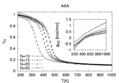
(Fig.1a) 1.: Temperature dependence of the helicity order parameter $q_{H}=<n_{H}>/(N-2)$ as obtained from simulations of polyalanine of chain length $N=10,15,20,30$ with ASA solvent representation. The free energy difference per residue $g_{hc}$ between helical and coil states is shown in the corresponding inlets.

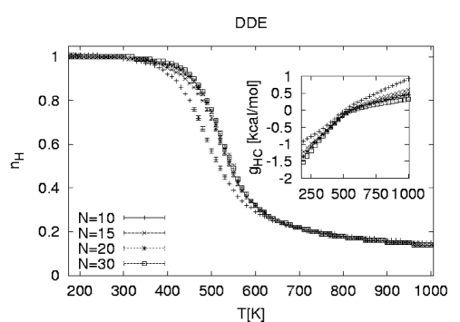
(Fig.1b) 2.: Temperature dependence of the helicity order parameter $q_{H}=<n_{H}>/(N-2)$ as obtained from simulations of polyalanine of chain length $N=10,15,20,30$ with DDE solvent. The free energy difference per residue $g_{hc}$ between helical and coil states is shown in the corresponding inlets.

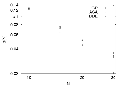
(Fig.2) 3.: Log-log plot of the nucleation parameter $\sigma$ as a function of the number of residues at $T=275$ K. The gas-phase values (GP) are taken from Ref. 2.

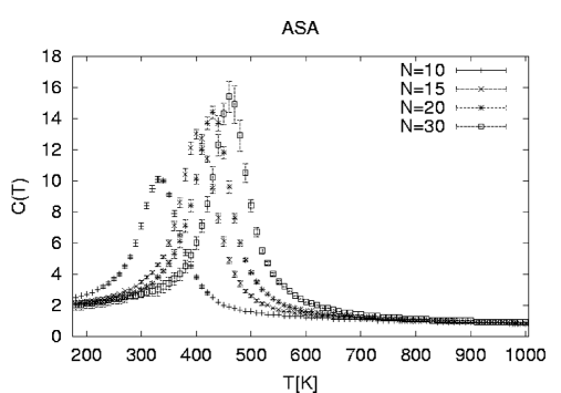
(Fig.3a) 4.: Specific heat $C(T)$ as a function of temperature $T$ for polyalanine molecules of chain length $N=10,15,20,$ and $30$ with ASA solvent representation.

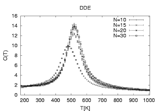
(Fig.3b) 5.: Specific heat $C(T)$ as a function of temperature $T$ for polyalanine molecules of chain length $N=10,15,20,$ and $30$ with DDE solvent representation.

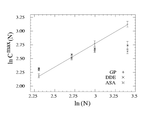
(Fig.4) 6.: Log-log plot of the peak value $C^{\rm max}(N)$ of the specific heat as a function of chain length $N$ for ASA and DDE simulations. For comparison, we show also the corresponding gas-phase values (GP) of Refs. 2,3 and the straight-line fit through them.

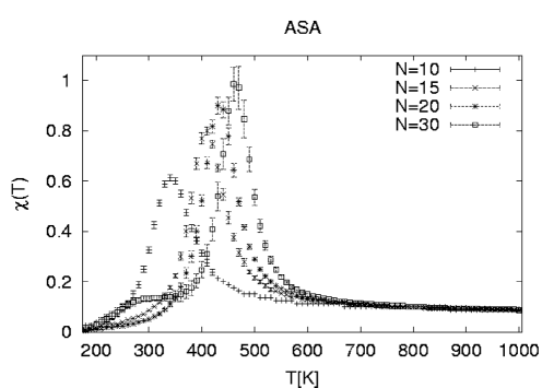
(Fig.5a) 7.: Susceptibility $\chi(T)$ as a function of temperature $T$ for polyalanine molecules of chain length $N=10,15,20,$ and $30$ with ASA solvent representation.

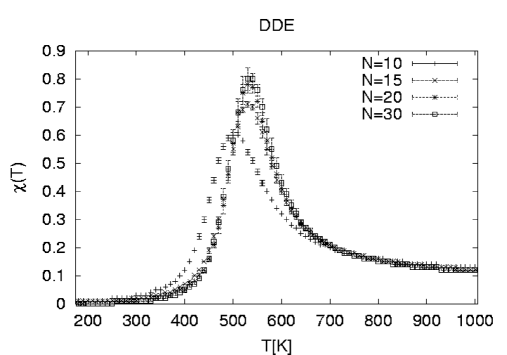
(Fig.5b) 8.: Susceptibility $\chi(T)$ as a function of temperature $T$ for polyalanine molecules of chain length $N=10,15,20,$ and $30$ with DDE solvent representation.

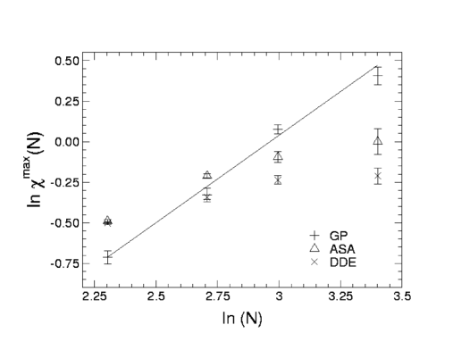
(Fig.6) 9.: Log-log plot of the peak value $\chi^{\rm max}(N)$ of the susceptibility as a function of chain length $N$ for ASA and DDE simulations. The corresponding gas-phase values (GP) of Ref. 2 and the straight-line fit through them are shown for comparison.

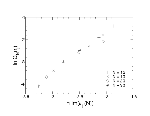
(Fig.7) 10.: Distribution of zeros for the polyalanine model with ASA solvent.

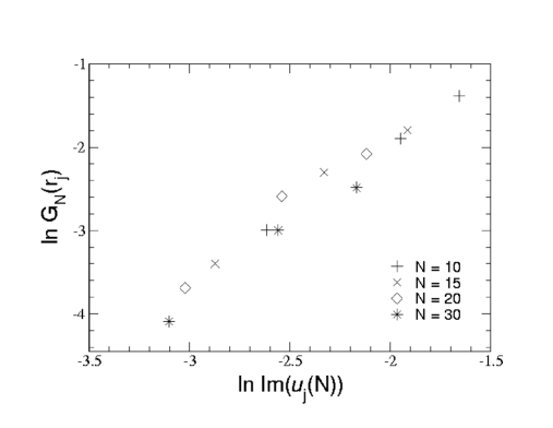
(Fig.8) 11.: Distribution of zeros for the polyalanine model with DDE solvent.

REFERENCES

- [1] D. Poland and H.A. Scheraga, Theory of Helix-Coil Transitions in Biopolymers (Academic Press, New York, 1970).
- [2] U.H.E. Hansmann and Y. Okamoto, J. Chem. Phys. 110, 1267 (1999); 111 1339(E) (1999).
- [3] N.A. Alves and U.H.E. Hansmann, Phys. Rev. Lett. 84, 1836 (2000).
- [4] N.A. Alves and U.H.E. Hansmann, Physica A 292, 509 (2001).
- [5] R.R. Hudgins, M.A. Ratner and M.F. Jarrold, J. Am. Chem. Soc. 120, 12974 (1998).
- [6] A. Mitsutake and Y. Okamoto, J. Chem. Phys. 112, 10638 (2000).
- [7] Y. Peng and U.H.E. Hansmann, Biophys. J. 82, 3269 (2002).
- [8] T. Ooi, M. Obatake, G. Nemethy, H.A. Scheraga, Proc. Natl. Acad. Sci. USA 8, 3086 (1987).
- [9] R. Lavery, H. Sklenar, K. Zakrzewska, B. Pullman, J. Biomol. Struct. & Dynamics 3, 989 (1986).
- [10] M.J. Sippl, G. Némethy, and H.A. Scheraga, J. Phys. Chem. 88, 6231 (1984), and references therein.
- [11] F. Eisenmenger, U.H.E. Hansmann, Sh. Hayryan, C.-K. Hu, Comp. Phys. Comm. 138, 192 (2001).
- [12] B. Hingerty, R.H. Richie, T.L. Ferrel, J. Turner, Biopolymers 24, 427 (1985).
- [13] U.H.E. Hansmann and Y. Okamoto, in: Stauffer, D. (ed.) “Annual Reviews in Computational Physics VI”,(Singapore: World Scientific), p.129. (1998).
- [14] U.H.E. Hansmann and Y. Okamoto, J. Comp. Chem. 14, 1333 (1993).
- [15] B.A. Berg and T. Neuhaus, Phys. Lett. B 267, 249 (1991).
- [16] Y. Okamoto and U.H.E. Hansmann, J. Phys. Chem. 99, 11276 (1995).
- [17] A.M. Ferrenberg and R.H. Swendsen, Phys. Rev. Lett. 61, 2635 (1988); Phys. Rev. Lett. 63, 1658(E) (1989), and references given in the erratum.
- [18] B.A. Berg, J. Stat. Phys. 82, 323 (1996).
- [19] N.A. Alves, J.P.N. Ferrite and U.H.E. Hansmann, Phys. Rev. E 65, 036110 (2002).
- [20] M.E. Fisher, in Lectures in Theoretical Physics, vol. 7c p.1 (University of Colorado Press, Boulder, 1965).
- [21] C. Itzykson, R.B. Pearson, and J.B. Zuber, Nucl. Phys. B 220 [FS8], 415 (1983).
- [22] P.N. Mortenson, D.A. Evans and D.J. Wales, J. Chem. Phys. 117, 1363 (2002).
- [23] J.A. Vila, D.R. Ripoll and H.A. Scheraga, Proc. Natl. Acad. Sci. USA 97, 13075 (2000).
- [24] Y. Levy, J. Jortner and O.M. Becker, Proc. Natl. Acad. Sci. USA 98, 2188 (2001).
- [25] B.H. Zimm and J.K. Bragg, J. Chem. Phys. 31, 526 (1959).
- [26] Chakrabartty, A.; R.L. Baldwin, R.L. In Protein Folding: In Vivo and In Vitro; Cleland J.; King, J. eds.; ACS Press: Washington, D.C., 1993; pp. 166–177.
- [27] N.A. Alves, J.R. Drugowich de Felicio and U.H.E. Hansmann, Int. J. Mod. Phys. C 8, 1063 (1997).
- [28] N.A. Alves, U.H.E. Hansmann and Y. Peng, Int. J. Mol. Sci. 3, 17 (2002).
- [29] W. Janke and R. Kenna, J. Stat. Phys. 102, 1211 (2001); Nucl. Phys. Proc. Supl. B106, 905 (2002); http://arXiv.org/abs/cond-mat/0103333; http://arXiv.org/abs/cond-mat/0208014.