Understanding correlated electron systems by a classification of Mott insulators

Abstract

This article surveys the physics of systems proximate to Mott insulators, and presents a classification using conventional and topological order parameters. This classification offers a valuable perspective on a variety of conducting correlated electron systems, from the cuprate superconductors to the heavy fermion compounds. Connections are drawn, and distinctions made, between collinear/non-collinear magnetic order, bond order, neutral spin 1/2 excitations in insulators, electron Fermi surfaces which violate Luttinger’s theorem, fractionalization of the electron, and the fractionalization of bosonic collective modes. Two distinct categories of $Z_{2}$ gauge theories are used to describe the interplay of these orders. Experimental implications for the cuprates are briefly noted, but these appear in more detail in a companion review article (S. Sachdev, cond-mat/0211005).

url]http://pantheon.yale.edu/~subir

1 Introduction

The foundations of solid state physics reside on a few simple paradigms of electron behavior which have been successfully applied and extended in a wide variety of physical contexts. The paradigms include the independent electron theory of Bloch, its more sophisticated formulation in Landau’s Fermi liquid theory, and the Bardeen-Cooper-Schrieffer (BCS) theory of electron pairing by an instability of the Fermi surface under attractive interactions between the electrons.

In the past decade, it has become increasingly clear that these paradigms are not particularly useful in understanding correlated electron systems such as the cuprate superconductors and the “heavy fermion” compounds. Many electrical and magnetic properties of these materials are rather far removed from those of the Fermi liquid, and remain poorly understood despite much theoretical work. The strong correlations between the electrons clearly makes the Fermi liquid an inappropriate starting point for a physical understanding of the many electron ground state.

One approach to the strong correlation problem, advocated here, is to begin at the point where the breakdown of the Bloch theory is complete: in the Mott insulator. These are materials in which Bloch theory predicts metallic behavior due to the presence of partially filled bands. However, the strong Coulomb repulsion between the electrons leads to dramatically different insulating behavior, often with a very large activation energy towards conduction. A key ingredient in our discussion here will be a classification of such Mott insulators: we will characterize the ground states of Mott insulators with a variety of “order parameters”. Some of these orders will have a conventional association with a symmetry of the Hamiltonian which is broken in the ground state, but others are linked to a more subtle ‘topological’ order [1].

An implicit assumption in our approach is that these same order parameters, or their closely related extensions, can also be used fruitfully in a description of other correlated systems, which may be either metallic or superconducting. In the latter systems, it is sometimes the case that the true long-range order characterizes only a proximate Mott insulator, and the order parameter ‘fluctuates’ at intermediate scales. In such a situation, the ground state and its elementary excitations are adiabatically connected to the Bloch/BCS states, but the order of the proximate Mott insulator is nevertheless important in understanding experiments, and especially those that explore correlations at mesoscopic scales. The theory of quantum phase transitions offers a powerful method for controlled predictions for such experiments: identify a quantum critical point associated with the onset of long-range order, and use it to expand back into the region with fluctuating order. The reader is referred to Ref. [2] for the application of such an approach to recent experiments in the cuprates.

With this motivation, let us turn to the central problem of the classification of Mott insulators. Newcomers to the Mott insulator problem should consult Section III of Ref. [2] at this point for an elementary introduction to the microscopic physics. The most important degrees of freedom in Mott insulators are the quantum spins $S_{\alpha}({\bf r})$, $\alpha=x,y,z$, which resides on the sites, ${\bf r}$, of some lattice. The states on each site transform under the spin $S$ representation of SU(2) (we are usually interested in $S=1/2$), and the sites are coupled together with the Hamiltonian

$$H=\sum_{{\bf r}<{\bf r}^{\prime}}J({\bf r},{\bf r}^{\prime})S_{\alpha}({\bf r})S_{\alpha}({\bf r}^{\prime})+\ldots,$$ (1)

where $J({\bf r},{\bf r}^{\prime})$ are short-range exchange interactions (usually all positive, realizing antiferromagnetic exchange), and the ellipses represent possible multiple spin couplings, all of which preserve full SU(2) spin rotation invariance. Here, and henceforth, there is an implied summation over repeated spin indices.

At the outset, it useful to distinguish Mott insulators by whether their ground states break the SU(2) spin rotation invariance of the Hamiltonian or not. The paramagnetic states have $\langle S_{\alpha}({\bf r})\rangle=0$ and preserve SU(2) spin rotation invariance, while the magnetically ordered states we consider break spin rotation invariance in the following simple manner

$$\langle S_{\alpha}({\bf r})\rangle={\rm Re}\left[\Phi_{\alpha}e^{i{\bf K}\cdot{\bf r}}\right];$$ (2)

here ${\bf K}$ is the ordering wavevector, while $\Phi_{\alpha}$ is a three-component complex order parameter; this order parameter transforms as a vector under spin rotations, while $\Phi_{\alpha}\rightarrow e^{-i{\bf K}\cdot{\bf a}}\Phi_{\alpha}$ under translations by a Bravais lattice vector ${\bf a}$. For simplicity we only consider systems with a single ordering wavevector, although the generalization to multiple wavevectors is not difficult.

The quantum theory of the magnetically ordered states has been well established for a long time: one considers slowly varying quantum fluctuations of the field $\Phi_{\alpha}$ in spacetime, and so obtains the Goldstone spin-wave excitations. Here, we wish to push the logic of this approach further: what happens when the quantum spin-wave fluctuations become strong enough to destroy the magnetic order in the ground state, and we reach a paramagnetic state with $\langle\Phi_{\alpha}\rangle=0$ ? We can think of this paramagnetic state as one with a ‘fluctuating’ $\Phi_{\alpha}$ order: does this tell us anything about the physical properties of the paramagnetic state ? We argue here that a surprising amount of information can gleaned from this seemingly naive approach, and it ultimately shows the way to a classification of both the magnetically ordered and the paramagnetic states.

1.1 Landau theory

We begin with the simple canonical procedure of considering the effective potential for $\Phi_{\alpha}$ fluctuations; our procedure here is general enough that it applies equally to both quantum and thermal fluctuations in insulators, metals, and superconductors. The structure of this effective potential is constrained by spin-rotation invariance and Bravais lattice translational symmetries, and the following low order terms are always allowed:

$$V(\Phi_{\alpha})=s\Phi_{\alpha}^{\ast}\Phi_{\alpha}+\frac{u}{2}\Phi_{\alpha}^{\ast}\Phi_{\beta}^{\ast}\Phi_{\alpha}\Phi_{\beta}+\frac{v}{2}\Phi_{\alpha}^{\ast}\Phi_{\alpha}^{\ast}\Phi_{\beta}\Phi_{\beta}$$ (3)

here $s$, $u$, $v$ are phenomenological Landau parameters ($u>0$, $v>-u$). If the value of ${\bf K}$ is commensurate with a reciprocal lattice vector, then additional low order terms can appear in the effective potential, but we defer considerations of such terms to later in this subsection.

As is usual, we begin with a minimization of $V$ over the values of the 3 complex numbers $\Phi_{\alpha}$. For $s>0$, we obtain the optimum value $\Phi_{\alpha}=0$, which obviously corresponds to the paramagnet. For $s<0$, we obtain two distinct classes of minima, which are not related to each other by any symmetry of the Hamiltonian. They are

$$({\rm A})~{}\mbox{\bf Non-collinear spins},~{}~{}v>0~{}~{}:~{}~{}\Phi_{\alpha}=n_{1\alpha}+in_{2\alpha}$$

$$~{}~{}~{}~{}~{}~{}~{}~{}~{}~{}~{}~{}~{}~{}~{}~{}~{}~{}~{}\mbox{with $n_{1,2\alpha}$ real, $n_{1\alpha}n_{2\alpha}=0$ and }n_{1\alpha}^{2}=n_{2\alpha}^{2}=\frac{-s}{2u}.$$

$$({\rm B})~{}\mbox{\bf Collinear spins},~{}~{}-u<v<0~{}~{}:~{}~{}\Phi_{\alpha}=e^{i\theta}n_{\alpha}$$

$$~{}~{}~{}~{}~{}~{}~{}~{}~{}~{}~{}~{}~{}~{}~{}~{}~{}~{}~{}~{}~{}~{}~{}~{}~{}~{}~{}~{}~{}~{}~{}\mbox{with $n_{\alpha}$ real and }n_{\alpha}^{2}=\frac{-s}{u+v}.$$ (4)

From (2) we can see easily that in case (B) the average values of the spins at all ${\bf r}$ are either parallel or antiparallel to each other, while in (A) the average spins values map out a circular spiral.

All the solutions in (A) or (B) represent physically distinct magnetically ordered ground states, but the states within a category are degenerate and can be transformed to each other by symmetries of the Hamiltonian. It is useful to more carefully specify the manifold of degenerate magnetically ordered ground states. For (A), the ground state manifold is easier to decipher by a different parameterization of $n_{1,2\alpha}$ which solves the constraints in (4):

$$n_{1\alpha}+in_{2\alpha}=\epsilon_{ac}z_{c}\sigma^{\alpha}_{ab}z_{b},$$ (5)

where $a,b$ extend over $\uparrow,\downarrow$, $\sigma^{\alpha}$ are the Pauli matrices, $\epsilon_{ab}$ is the antisymmetric tensor, and $z_{a}$ is a two-component complex field with $|z_{\uparrow}|^{2}+|z_{\downarrow}|^{2}=\sqrt{-s/2u}$; note that $z_{\alpha}$ transforms like a $S=1/2$ spinor under spin rotations, while

$$z_{a}\rightarrow e^{-i{\bf K}\cdot{\bf a}/2}z_{a},$$ (6)

under translation by a Bravais lattice vector ${\bf a}$. It is easy to check that (5) is in fact the most general solution of the constraints for case (A) in (4), but with a two-fold redundancy: $z_{a}$ and $-z_{a}$ correspond to the same non-collinear ground state. The two complex numbers $z_{a}$ are equivalent to four real numbers, and hence the manifold of ground states is $S_{3}/Z_{2}$, where $S_{3}$ is the three-dimensional surface of a sphere in four dimensions. Turning to (B), $n_{\alpha}$ maps out the surface of an ordinary sphere, $S_{2}$, while the phase factor $e^{i\theta}$ is U(1)$\cong S_{1}$, a circle. However the factorization of $\Phi_{\alpha}$ into $n_{\alpha}$ and $e^{i\theta}$ is redundant because we can map $n_{\alpha}\rightarrow-n_{\alpha}$ and $\theta\rightarrow\theta+\pi$ without changing $\Phi_{\alpha}$; hence the manifold of ground states for (II) is $(S_{2}\times S_{1})/Z_{2}$. Summarizing, we have

$$({\rm A})~{}\mbox{\bf Non-collinear spins},~{}~{}\mbox{ground state manifold = }S_{3}/Z_{2};$$

$$({\rm B})~{}\mbox{\bf Collinear spins},~{}~{}\mbox{ground state manifold = }(S_{2}\times S_{1})/Z_{2}.$$ (7)

This is a good point to mention additional restrictions that are placed on the ground state manifold at special commensurate values of ${\bf K}$. These arise for ${\bf K}$ such that $2p{\bf K}$ equals a reciprocal lattice vector, where $p$ is an integer. Then from the transformation of $\Phi_{\alpha}$ under Bravais lattice translations we observe that the effective potential can contain the additional term

$$V_{\rm comm}=-w\left(\Phi_{\alpha}\Phi_{\alpha}\right)^{p}+\mbox{c.c.}$$ (8)

For case (B) it is easy to see from (4) and (8) that $V_{\rm comm}$ acts only on the angular field $\theta$, and selects $2p$ values of $\theta$ in the ground state. So the order parameter manifold is now reduced to $(S_{2}\times Z_{2p})/Z_{2}$: this change in the manifold has important consequences for $p=1$, but is not of particular importance at larger values of $p$. For case (A), it follows from (4) and (8) that $V_{\rm comm}$ has no influence on the ground state energy, and that the order parameter manifold remains $S_{3}/Z_{2}$.

Having laid the ground work, and now are ready to extend this simple understanding of magnetically ordered states to paramagnetic phases, where the order parameter $\Phi_{\alpha}$, constrained as in (4), is fluctuating. As we will see, global aspects of the order parameter manifold in (7) will play a crucial role. We will consider case (A) with non-collinear spins in Section 2, while case (B) with collinear spins will be discussed in Section 3. In both cases we will attempt to understand a variety of phases, including insulators, metals, and superconductors. The evidence so far indicates that the cuprate superconductors are in category (B), and this is discussed at some length in Ref. [2]. Some of the more exotic phases appear in category (A), and we anticipate these will find realizations in heavy-fermion compounds, and particularly in those in which the magnetic moments reside on frustrated lattices such as the pyrochlore or the triangular.

2 Noncollinear spins

An understanding of $\Phi_{\alpha}$ fluctuations in the paramagnetic phase requires that we proceed beyond the simple effective potential in (3), and consider spacetime dependent fluctuations using a suitable effective action. We assume that the non-collinearity of the spin correlations is imposed at some short scale, and so at longer scales we wish to impose the constraints under (A) in (4) at the outset in our effective action. This is most conveniently done using the parameterization in (5). We discretize spacetime on some regular lattice of sites $j$ on which we have the spinors $z_{ja}$: note that this lattice may have little to do with the lattice of sites on which the underlying spins reside, and that we are working here on a coarse-grained scale. Any effective action on this coarse-grained lattice must be invariant under global spin rotations, and also under the global lattice transformation (6). However, most importantly, we note from (5) that it must also be invariant under the $Z_{2}$ gauge transformation

$$z_{ja}\rightarrow\varepsilon_{j}z_{ja}$$ (9)

where $\varepsilon_{j}=\pm 1$ is a spacetime dependent field which generates the gauge transformation. This transformation is permitted because the local physics can only depend upon the order parameter $\Phi_{\alpha}$, which is invariant under (9).

We begin in Section 2.1 by considering a very simple model of $z_{ja}$ fluctuations. This model is surely an oversimplification for the complex quantum systems of interest here, but it will at least allow us to obtain an initial understanding of possible phases and the global structure of the phase diagram. We will discuss applications to realistic physical systems in Section 2.2.

2.1 Simple effective action

Our model here omits long-range interactions and mobile excitations that can carry charge, which implies that it could apply directly only to insulators. We also neglect all Berry phases associated with the underlying spins. This will allow us to at least obtain a first understanding of the possible phases and the global structure of the possible phase diagrams. More careful considerations, described partly in Section 3.1 below, show that the Berry phases are crucial for realizing that ‘bond order’ is present in the ‘confining’ phase to be discussed shortly, but that they can be safely neglected in the other phases. The presentation below is based upon results contained in Refs. [3, 4, 5, 6].

With the above caveats, we initially introduce the following simple partition function:

$$\mathcal{Z}_{z} = \int\prod_{j}dz_{ja}dz^{\ast}_{ja}\delta\left(\left|z_{ja}\right|^{2}-1\right)\exp\left(-\mathcal{S}_{z}\right)$$

$$\mathcal{S}_{z} = -\widetilde{J}_{1}\sum_{\langle ij\rangle}z^{\ast}_{ia}z_{ib}z^{\ast}_{jb}z_{ja}-\widetilde{J}_{2}\sum_{\langle ij\rangle}\left(z^{\ast}_{ia}z^{\ast}_{ib}z_{ja}z_{jb}+\mbox{c.c.}\right)+\ldots,$$ (10)

where we have rescaled the $z_{ja}$ fields so that they obey the unit length constraint on every site $j$, and $\langle ij\rangle$ represents nearest neighbors. The terms shown in (10) constitute the most general coupling between two sites consistent with the symmetries discussed above. Note that at this order the discrete symmetry (6) has effectively restricted us to terms which are also invariant under the U(1) symmetry $z_{ja}\rightarrow e^{i\varphi}z_{ja}$ with $\varphi$ arbitrary: so the model $\mathcal{S}_{z}$ has a global SU(2)$\times$U(1) symmetry.

While it is possible to proceed with (10), the full spectrum of possible phases is seen more easily by a representation which makes the $Z_{2}$ gauge invariance more explicit. For this, we must introduce a $Z_{2}$ gauge field $\sigma_{ij}=\pm 1$, which resides on the links of the lattice, and which obeys the mapping

$$\sigma_{ij}\rightarrow\varepsilon_{i}\sigma_{ij}\varepsilon_{j}$$ (11)

under the gauge transformation in (9). We can loosely view $\sigma_{ij}$ as arising from a Hubbard-Stratonovich decoupling of the quartic terms in (10). With $\sigma_{ij}$ in hand, we can now propose the alternative action as $Z_{2}$ gauge theory

$$\mathcal{Z}_{\rm noncoll} = \int\prod_{j}dz_{ja}dz^{\ast}_{ja}\delta\left(\left|z_{ja}\right|^{2}-1\right)\sum_{\{\sigma_{ij}=\pm 1\}}\exp\left(-\mathcal{S}_{\rm noncoll}\right)$$

$$\mathcal{S}_{\rm noncoll} = -J_{1}\sum_{\langle ij\rangle}z_{ia}^{\ast}\sigma_{ij}z_{ja}+\mbox{c.c.}-K\sum_{\Box}\prod_{\langle ij\rangle\in\Box}\sigma_{ij}-J_{2}\sum_{\langle ij\rangle}z^{\ast}_{ia}z_{ib}z^{\ast}_{jb}z_{ja}.$$ (12)

The second term is the sum of the products of $\sigma_{ij}$ over all elementary plaquettes of the lattice—it is the standard Maxwell term for a $Z_{2}$ gauge field. The first term proportional to $J_{1}$ is easily seen to have a global O(4) symmetry of rotations on the order parameter manifold $S_{3}$. This symmetry is not present in the underlying spin model, and so we have added the last term proportional to $J_{2}$ which reduces the symmetry down to the required SU(2)$\times$U(1). For $K=0$, we can freely sum over the $\sigma_{ij}$ independently on each link, and the resulting action is easily seen to have a structure identical to $\mathcal{S}_{z}$ in (10). For large $K$, the action (12) will allow us to easily access states which would have been harder to extract from (10).

What is the physical significance of the flux in the $Z_{2}$ gauge field which is controlled by the coupling $K$ in (12) ? It is a measure of the location of defects associated with the homotopy group $\pi_{1}(S_{3}/Z_{2})=Z_{2}$, now often called ‘visons’ [7]. Upon encircling a vison in a closed loop, the values of $z_{a}$ change smoothly along the loop, but the initial and final values of $z_{a}$ reside on polar opposite points on $S_{3}$; all physical energies are independent of this sign change, and so there is no practical significance to this cut (see Fig 1).

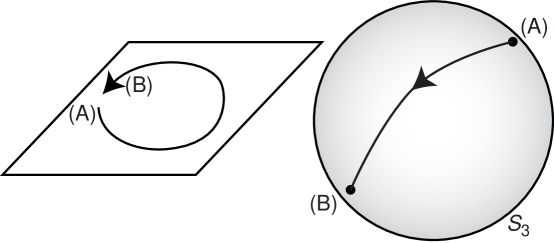
Figure 1: A vison defect associated with $\pi_{1}(S_{3}/Z_{2})=Z_{2}$. The left hand side represents a two-dimensional section of spacetime, while the right hand side is the space of points $z_{a}$ which reside on $S_{3}$. Polar opposite points on $S_{3}$ are represented by A and B. The $Z_{2}$ gauge field $\sigma_{ij}=1$ along the loop, but $\sigma_{ij}=-1$ on the link directly connecting A and B. There is a $Z_{2}$ gauge flux at the center of the vison, and this flux allows identification of the vison defect even when the $z_{a}$ are fluctuating, and there is no magnetic order.

From (12) we see that the action will be minimized by $\sigma_{ij}=1$ along the loop, but we prefer $\sigma_{ij}=-1$ across the cut between the initial and final points . Measuring the $Z_{2}$ flux associated with this configuration of $\sigma_{ij}$, we conclude that the flux resides in a small region at the center of the vison.

We can now sketch a phase diagram of $\mathcal{S}_{\rm noncoll}$ in the $J_{1},K$ plane in 2+1 spacetime dimensions (related considerations apply to higher spacetime dimensions). Many important features follow immediately by an analogy with a simpler problem considered by Lammert et al. [8, 9] in the entirely different context of liquid crystals: they examined a problem with an order parameter belonging to the space $S_{2}/Z_{2}$ (in contrast to the $S_{3}/Z_{2}$ order parameter of interest here), which also permits an effective action in a $Z_{2}$ gauge theory very similar to $\mathcal{S}_{\rm noncoll}$. Using their results, and those of the earlier work of Refs. [10, 11], we obtain the phase diagram for 2+1 spacetime dimensions shown in Fig 2.

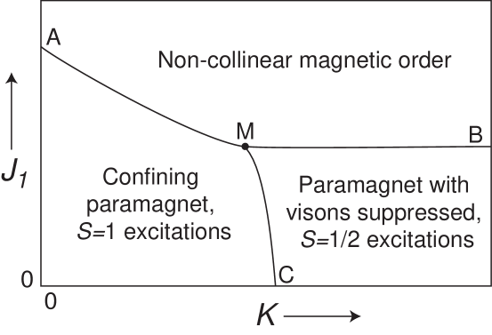
Figure 2: Schematic phase diagram of the model $\mathcal{S}_{\rm noncoll}$ in (12) as a function of $J_{1}$ and $K$ in 2+1 spacetime dimensions. We assume that $J_{2}$ takes a small positive value. The model $\mathcal{S}_{\rm noncoll}$ describes some of the physics of Mott insulators with non-collinear spin correations. However it omits Berry phase terms which impose the Heisenberg commutation relations of the spins in (1). These Berry phases play an important role in the small $K$ region of the phase diagram: they induce bond order in the confining paramagnet, along with additional intermediate phases. The influence of the Berry phases is studied in Section 3.1 and in Ref. [12]. The suppression of visons in the deconfined state at large $K$ is interpreted as a ‘topological’ order.

Consider first the physics near the line $K=0$. Here we can simply sum over the $\sigma_{ij}$, and work instead with the original action $\mathcal{S}_{z}$ in (10). At large $J_{1}$ we have a conventional non-collinear magnetically ordered phase with $\langle z_{a}\rangle\neq 0$, and hence $\langle\Phi_{\alpha}\rangle\neq 0$. With decreasing $J_{1}$, there is a phase transition to a paramagetic phase. The key to understanding the nature of this paramagnetic phase, and of the quantum phase transition, is the observation that $\mathcal{S}_{z}$ contains only gauge-invariant bilinears in $z_{ja}$ on each site, and so we should be able to describe the physics in terms of the bilinear fields $n_{1,2\alpha}$ in (5). Alternatively stated, the strong $Z_{2}$ gauge fluctuations (and the accompanying proliferation of visons) has confined the $z_{a}$ quanta, and the elementary excitations of the paramagnetic state are the $n_{1,2\alpha}$ quanta. Notice that these fields carry spin $S=1$, and so the paramagnetic phase is a confining state with only integer spin excitations. The quantum transition between the magnetically ordered state and this confining state, along the line AM in Fig 2 can be addressed by continuum models expressed directly in terms of the $n_{1,2\alpha}$. This has been done by Kawamura [13], Pelissetto et al. [14, 15], and Calabrese et al. [16] in the context of classical phase transitions in stacked triangular lattices, and they obtained a continuous phase transition in the “chiral” universality class in 2+1 spacetime dimensions. The global symmetry at this “chiral” fixed point remains SU(2)$\times$U(1).

Let us turn now to the physics near the line $J_{1}=0$ in Fig 2. Here, the $z_{a}$ fluctuate strongly and can be integrated out, leading to a pure $Z_{2}$ gauge theory in the $\sigma_{ij}$. In 2+1 spacetime dimensions, this gauge theory is well known [10, 11] to have a confinement-deconfinement transition at some critical $K$ near the point C: the large $K$ region is the deconfined state where vison fluxes are suppressed. Consequently, in this deconfined state, we can use a simple physical picture in which we choose a gauge with all $\sigma_{ij}=1$: the $z_{a}$ quanta in (12) are then free to propagate through the system. The large $K$, small $J_{1}$ region is therefore a paramagnetic state with neutral $S=1/2$ ‘spinon’ excitations. The suppression of visons in this state is interpreted as the presence of ‘topological order’; this is similar to the topological order below the Kosterlitz-Thouless transition in the two-dimensional classical XY model, where point vortices are suppressed [1].

Finally, to complete our picture of the phase diagram, we look at the region of large $K$. Here, visons are suppressed, and so we can freeze $\sigma_{ij}=1$, and we are left with a simple model of interacting $z_{\alpha}$ quanta, with a global SU(2)$\times$U(1) symmetry. Such a theory has been studied in its continuum limit, and yields a description of the magnetic ordering transition along the line BM: the critical point has a large O(4) symmetry in 2+1 spacetime dimensions, and the critical exponents are those of the 4-component $\varphi^{4}$ field theory [17, 5].

2.2 Physical Applications

The results of Section 2.1 for large $K$ apply directly to Mott insulators with non-collinear spin correlations. The mapping of the magnetically ordered phase is evident, while we identify the paramagnet with visons suppressed with the resonating valence bond (RVB) state of Refs [18, 19, 20, 21, 22, 23]. The latter identification follows from the full preservation of symmetries of the Hamiltonian, the presence of neutral $S=1/2$ spinon excitations, and from the topological order implied by the suppression of visons [3, 22, 7]. Experimentally, we note that the evidence for a RVB state in Cs₂CuCl₄ [24] is in a system with non-collinear spin correlations, consistent with our theoretical picture. At small $K$, and smaller $J_{1}$, the proliferation of visons requires more care, as the quantum mechanics of the underlying spins contributes a Berry phase to each vison [25, 7]. These phases induce bond order in the confining paramagnet, and can also lead to additional intermediate states [7, 12]: we will not discuss this further here, but will illustrate the influence of Berry phases in the simpler context of collinear spins in Section 3.1.

Let us finally move away from the Mott insulator, and introduce mobile charge carriers into the RVB state just discussed, by doping in holes. A scenario which has been intensively discussed in the literature [20, 21, 7] is that hole fractionalizes into independent quasiparticle excitations: a neutral $S=1/2$ ‘spinon’ and a spinless, charge $e$ holon. The spinon here is, of course, that just discussed above here in the proximate Mott insulator. We can express this fractionlization of the injected hole by the following schematic operator relation for the electron annihilation operator $c_{a}$:

$$c_{a}=f^{\dagger}\left(\lambda_{1}z_{a}+\lambda_{2}\epsilon_{ab}z_{b}^{\ast}\right),$$ (13)

where $z_{a}$ is the bosonic neutral spinon operator from Section 2.1, $f^{\dagger}$ is a fermionic operator that creates a spinless hole, and $\lambda_{1,2}$ are constants that depend upon the details of the microscopic physics. It is possible for the fermionic statistics to pass from the hole to the spinon by binding between quasiparticles and visons, as has been discussed in some detail in Refs. [26, 27, 28]. Then the relationship (13) would be replaced by

$$c_{a}=b^{\dagger}\left(\lambda_{3}f_{a}+\lambda_{4}\epsilon_{ab}f^{\dagger}_{b}\right),$$ (14)

where $f_{a}$ is a neutral, $S=1/2$, fermionic spinon, $b$ is charge $e$ bosonic holon, and $\lambda_{3,4}$ are constants. In this scenario, the Bose condensation of the holon leads to a BCS superconductor with vestiges of the topological order of the RVB Mott insulator: experimental probes of this ‘fluctuating’ topological order have been proposed [29, 30, 31, 2], but no positive signal has been observed so far in the cuprates [32, 33].

2.2.1 Fractionalized Fermi liquids

It has been argued recently [34, 35] that a different possibility is more likely for the doped RVB Mott insulator in $d\geq 2$ spatial dimensions. The doped electrons (or holes), instead of fractionalizing into spinless charged particles and neutral $S=1/2$ spinons, retain their integrity in the ground state, and their spin and charge remain bound to each other. At the same time, the neutral $S=1/2$ spinons of the RVB Mott insulator survive in the doped system, and are only renormalized slightly by the mobile carriers. So, alternatively stated, the added electrons form a Fermi-liquid-like state which is approximately decoupled from the spinons. The resulting metallic state has a Fermi surface with $S=1/2$, charge $-e$ quasiparticle excitations, along with a separate set of neutral spinon excitations which continue from the RVB Mott insulator. Moreover, the volume enclosed by the Fermi surface is ‘small’ i.e. it is determined solely by the density of doped electrons, and does not include the spins of the Mott insulator. In this situation, the volume of the Fermi surface becomes a direct experimental signal of the topological order in the RVB state. Heavy fermion compounds on frustrated lattices with weak or absent magnetic order are likely candidates for realizing this state.

The fractionalized Fermi liquid defined above violates the standard Luttinger theorem, and it is useful to express this violation in its most general terms. Consider a correlated electron system on a periodic lattice in $d$ spatial dimensions, whose ground state preserves time-reversal and spin rotation invariance, and has unit cell volume $v_{0}$. Let $n_{T}$ be the total density of electrons per volume $v_{0}$; $n_{T}$ includes all the electrons in the system, including e.g. the core 1s electrons. Luttinger’s theorem states that in a conventional Fermi liquid state

$$2\times\frac{v_{0}}{(2\pi)^{d}}\times\left(\mbox{Volume enclosed by Fermi surface}\right)=n_{T}(\mbox{mod 2}).$$ (15)

The leading factor of 2 on the left hand side comes from spin degeneracy, while modulus 2 on the right hand side allows fully filled bands to not contribute to the Fermi surface volume. The fractionalized Fermi liquid being discussed here violates (15), but instead obeys a modified relation

$$2\times\frac{v_{0}}{(2\pi)^{d}}\times\left(\mbox{Volume enclosed by Fermi surface}\right)=(n_{T}-1)(\mbox{mod 2}).$$ (16)

So exactly one electron per unit cell has dropped out from the Fermi volume. This can only happen in a topologically ordered state which possesses neutral $S=1/2$ spinon excitations, in addition to the electron-like quasiparticle excitations on the small Fermi surface.

3 Collinear spins

We turn here to the second broad category of correlated electron systems introduced in Section 1: the collinear spin case (B) in (4). We will find that the paramagnetic states with fluctuating collinear spin order are entirely different from those present for non-collinear spins in Section 2.2. The order parameter manifold, from (7) is now $(S_{2}\times S_{1})/Z_{2}$, and the appearance of a $Z_{2}$ quotient means that the physics can again be described in a generalized phase diagram of a $Z_{2}$ gauge theory [36]. However, the $Z_{2}$ flux now identifies a new type of defect which we will discuss in Section 3.2. The $Z_{2}$ gauge theory also has a deconfined phase, but this $Z_{2}$ fractionalization does not lead to neutral $S=1/2$ excitations; instead, as we will see in Section 3.2 it is the spin and charge collective modes which ‘fractionalize’ apart from each other.

A separate crucial property of Mott insulators with collinear spin correlations in spatial dimension $d=2$ is the ubiquity of confining states with only integer spin excitations [37]. Moreover, except for certain special values of the spin $S$ per unit cell, these confining states break lattice space group symmetries by the appearance of spontaneous ‘bond order’ in the ground state. This bond order also often survives in proximate conducting states obtained by doping the Mott insulator [4, 38]. Let us define bond order more precisely here: most generally, bond order implies a modulation in observables invariant under spin rotation and time reversal which break a space group symmetry of the Hamiltonian. The simplest such observable in states proximate to Mott insulators is simply the spin exchange energy: so we can introduce the bond order parameter

$$Q_{\bf a}({\bf r})=\langle S_{\alpha}({\bf r})S_{\alpha}({\bf r}+{\bf a})\rangle,$$ (17)

where ${\bf a}$ is usually a vector connecting near neighbors. Note that for ${\bf a}=0$, $Q_{0}({\bf r})$ is a measure of the charge density on site ${\bf r}$, and so (if permitted by the symmetry of the state) there is usually also a modulation of the site charge density in a bond-ordered state. However, we expect the long-range Coulomb interactions to suppress modulations at ${\bf a}=0$, while those with ${\bf a}\neq 0$ should be significantly larger.

We will begin our discussion in Section 3.1.1 by a detailed discussion of the simplest, and most common, Mott insulator with collinear spin correlations: that on a $d$-dimensional cubic lattice with ordering wavevector ${\bf K}=(\pi,\pi,\ldots)$. This order is commensurate with $p=1$, in the notation of (8). We will explicitly evaluate the quantum spin Berry phases for this case, show their intimate connection to bond order. Section 3.1.2 will also include extensions of the study of bond order to doped systems with mobile carriers.

States at other wavevectors and in metals and superconductors, and the $Z_{2}$ gauge theory of the fractionalization of their excitations will be discussed in Section 3.2.

3.1 Berry phases and bond order

3.1.1 Mott insulators

Consider the insulating antiferromagnetic (1) on a $d$-dimensional cubic lattice with predominant nearest-neighbor exchange interactions. This should have collinear spin correlations with ${\bf K}=(\pi,\pi,\ldots)$, which allows the term with $p=1$ in (8). Inserting $\Phi_{\alpha}=e^{i\theta}n_{\alpha}$ (obtained from (4)) into (8) we observe that we can always choose the origin of co-ordinates so that the values $\theta=0,\pi$ are preferred. These do not lead to new values of $\Phi_{\alpha}$, and so in this case we have simply $\Phi_{\alpha}=n_{\alpha}$, a real three-component vector.

Now express the coherent state path integral of (1) using the values of the field $n_{\alpha}$ on a $d+1$ dimensional hypercubic lattice discretization of spacetime. The derivation of this path integral is reviewed in Chapter 13 of Ref. [39], and leads to the following partition function

$$\mathcal{Z}_{n}=\int\prod_{j}dn_{j\alpha}\delta(n_{j\alpha}^{2}-1)\exp\left(-\frac{1}{2g}\sum_{\langle ij\rangle}n_{i\alpha}{n}_{j\alpha}-iS\sum_{j}\eta_{j}\mathcal{A}_{j\tau}\right),$$ (18)

where $i,j$ are sites of the $d+1$ dimensional hypercubic lattice (the symbol $i=\sqrt{-1}$ in the prefactor of the second term, and the context should prevent confusion on its meaning), and we have rescaled all the $n_{j\alpha}$ to make them unit length. The first term in the action above is the analog of the terms in (10), and imposes a cost in the action for deviations from the perfectly ordered state; we expect a magnetically ordered state $\langle n_{\alpha}\rangle\neq 0$ for small values of the coupling $g$, and a paramagnetic state with $\langle n_{\alpha}\rangle=0$ for large $g$. The second term in (18) is the all important Berry phase: here $\eta_{j}=e^{i{\bf K}\cdot{\bf r}_{j}}=\pm 1$ is a fixed field identifying the spatial sublattice of the site $j$ (note that $\eta_{j}$ is independent of the imaginary time co-ordinate, $\tau$). Finally $\mathcal{A}_{j\mu}$, with $\mu=\tau,x,y,\ldots$ taking $d+1$ dimensional possible values, is defined by

$$\mathcal{A}_{j\mu} \equiv$$ oriented area enclosed by the spherical triangle with vertices (19)

$$~{}\mbox{$n_{j\alpha}$, $n_{j+\hat{\mu},\alpha}$, and any {\em fixed} reference $N_{0\alpha}$},$$

where $j+\hat{\mu}$ is the nearest site to $j$ in the $\mu$ direction. It is customary to choose $N_{0\alpha}=(0,0,1)$, the north pole, but it is not difficult to see that the partition function $\mathcal{Z}_{n}$ is independent of the value of $N_{0\alpha}$. Indeed, elementary geometric considerations of spherical triangles show [12] that a choice of a different $N_{0\alpha}^{\prime}$ leads to $\mathcal{A}_{j\mu}^{\prime}$ which is related to $\mathcal{A}_{j\mu}$ by a ‘gauge transformation’

$$\mathcal{A}_{j\mu}^{\prime}=\mathcal{A}_{j\mu}-\Delta_{\mu}\phi_{j}$$ (20)

where $\Delta_{\mu}$ is the discrete lattice derivative in the $\mu$ direction, and $\phi_{j}$ is the area of the spherical triangle formed by $n_{j\alpha}$, $N_{0\alpha}$ and $N_{0\alpha}^{\prime}$. It should also be noted here that the area of a spherical triangle is uncertain modulo $4\pi$, and so is the value of $\mathcal{A}_{j\mu}$, but the partition function $\mathcal{Z}_{n}$ is insensitive to this uncertainty because $e^{i4\pi S}=1$.

For small $g$ in $\mathcal{Z}_{n}$, fluctuations of $n_{\alpha}$ are suppressed, and in dimensions $d>1$, we are in the conventional Néel ordered ground state with $\langle n_{\alpha}\rangle\neq 0$. As an aside, we note the small $g$ behavior for $d=1$. In $d=1$ we can continue to assume that $n_{\alpha}$ varies smoothly from site-to-site for small $g$, and hence take the naive continuum limit of (18). This yields the O(3) non-linear sigma model in 1+1 dimensions, along with a topological $\theta$-term with co-efficient $\theta=2\pi S$, as reviewed in Ref. [39]. For integer $S$ this exhibits the Haldane gap state, while for half-odd-integer $S$ a gapless critical state as in the Bethe’s solution of the nearest neighbor antiferromagnetic chain can appear.

Our interest here is primarily in the larger $g$ regime of $\mathcal{Z}_{n}$, where there are significant fluctuations of $n_{\alpha}$, and we are in a paramagnet with $\langle n_{\alpha}\rangle=0$. There are large fluctuations here in the value of the $\mathcal{A}_{j\mu}$ also, and so the Berry phase term requires careful evaluation. An explicit evaluation of this term is essentially impossible, but considerable progress has been made in the ‘easy-plane’ case, where spin-anisotropies reduce fluctuations to the equator in spin space with $n_{j\alpha}=(\cos\theta_{j},\sin\theta_{j},0)$ [12]. Here we follow a simple ‘hand-waving’ argument [40] whose results are known to be consistent with all cases in which more sophisticated methods are possible; the paragraph below is partly reproduced from the review in Ref. [40], to which we will also refer the reader for additional details.

The main idea for the larger $g$ regime is to change variables from the order parameter $n_{j\alpha}$ to the field $\mathcal{A}_{j\mu}$ which naturally represents the Berry phase. Formally, this can be done by introducing new ‘dummy’ variables $A_{j\mu}$ and rewriting (18) by introducing delta-function factors which integrate to unity on each link; this leads to

$$\mathcal{Z}_{n} = \int\prod_{j\mu}dA_{j\mu}\exp\left(-i2S\sum_{j}\eta_{j}A_{j\tau}\right)\int\prod_{j}dn_{j\alpha}\delta(n_{j\alpha}^{2}-1)\delta(\mathcal{A}_{j\mu}/2-A_{j\mu})$$ (21)

$$~{}~{}~{}~{}~{}~{}~{}~{}~{}~{}~{}~{}~{}~{}~{}~{}~{}~{}~{}~{}~{}~{}~{}~{}~{}~{}~{}~{}~{}~{}~{}~{}~{}~{}~{}~{}~{}~{}~{}~{}\times\exp\left(-\frac{1}{2g}\sum_{\langle ij\rangle}n_{i\alpha}{n}_{j\alpha}\right)$$

$$= \int\prod_{j\mu}dA_{j\mu}\exp\left(-\mathcal{S}_{A}(A_{j\mu})-i2S\sum_{j}\eta_{j}A_{j\tau}\right).$$

In the first expression, if the integral over the $A_{j\mu}$ is performed first, we trivially return to (18); however in the second expression we perform the integral over the $n_{j\alpha}$ variables first at the cost of introducing an unknown effective action $\mathcal{S}_{A}$ for the $A_{j\mu}$. In principle, evaluation of $\mathcal{S}_{A}$ may be performed order-by-order in a “high temperature” expansion in $1/g$: we match correlators of the $A_{j\mu}$ flux with those of the $\mathcal{A}_{j\mu}$ flux evaluated in the integral over the $n_{j\alpha}$ with positive weights determined only by the $1/g$ term in (18). Rather than undertaking this laborious calculation, we can guess essential features of the effective action $\mathcal{S}_{A}$ from some general constraints. First, correlations in the $n_{j\alpha}$ decay exponentially rapidly for large $g$ (with a correlation length $\sim 1/\ln(g)$), and so $\mathcal{S}_{A}$ should be local. Second, (20) implies that $\mathcal{S}_{A}$ should be invariant under the gauge transformation

$$A_{j\mu}^{\prime}=A_{j\mu}-\Delta_{\mu}\phi_{j}/2.$$ (22)

Finally, uncertainity of $\mathcal{A}_{j\mu}$ modulo $4\pi$ implies that $\mathcal{S}_{A}$ should also be invariant under

$$A_{j\mu}\rightarrow A_{j\mu}+2\pi.$$ (23)

The simplest local action which is invariant under (22) and (23) is that of compact U(1) quantum ‘electrodynamics’ and so we propose that for larger values of $g$, $\mathcal{Z}_{n}\approx\mathcal{Z}_{A}$ with

$$\mathcal{Z}_{A}=\int\prod_{j\mu}dA_{j\mu}\exp\left(\frac{1}{e^{2}}\sum_{\Box}\cos\left(\Delta_{\mu}A_{j\nu}-\Delta_{\nu}A_{j\mu}\right)-i2S\sum_{j}\eta_{j}A_{j\tau}\right);$$ (24)

comparison with the large $g$ expansion shows that the coupling $e^{2}\sim g^{2}$. This is one of the central results of this subsection [37, 41, 42, 12]: the paramagnetic state of a Mott insulator with two-sublattice collinear spin correlations in $d$ spatial dimensions is described by a compact U(1) gauge theory in $d+1$ spacetime dimensions, accompanied by a Berry phase term as specified in (24). In the gauge theory/particle physics language, the Berry phase corresponds to static ‘matter’ fields of charge $\pm 2S$ residing on the two spatial sublattices of the $d$-dimensional lattice.

We are now faced with the technical problem of evaluating the partition function of compact QED in $d+1$ spacetime dimensions in the presence of static background matter fields, as written in (24). There is a good understanding of the phases of this theory in $d=1,2$, and the reader is referred to another review [40] for further details—here we will summarize the main conclusions. The structure in $d=3$ is not yet fully understood, and this remains an important avenue for future research. All of these previous analyses rely on a duality mapping of (24); the mapping proceeds in a canonical manner, beginning with a rewriting of the cosine term in (24) in the Villain periodic Gaussian form, followed by the evaluation of the integral over the $A_{j\mu}$, which results in a partition function of ‘dual’ fields. The advantage of this duality mapping is that the Berry phases are exactly accounted for at the outset, and the partition function in the dual representation has only positive weights—this makes it amenable to standard analyses of statistical field theory. A discussion of the results in various spatial dimensions, $d$, follows.

In $d=1$, the duality mapping of the Villain form of $\mathcal{Z}_{A}$ leads to a simple partition function that can be evaluated exactly [40, 12]. There is a gap to all excitations, and for half-odd-integer $S$ a two-fold degenerate ground state and a broken translational symmetry associated with the appearance of bond order, as illustrated in Fig 3.

Figure 3: Schematic representation of the ground state of $\mathcal{Z}_{A}$ for half-odd-integer $S$ in $d=1$. The state is identified with the different values of $Q_{\bf a}({\bf r})$ in (17) with ${\bf a}$ a nearest neighbor vector: the links with ellipses have values of $Q_{{\bf a}}({\bf r})$ distinct from those without. The reader can also view this picture as caricature of the wavefunction—a simple trial state for $S=1/2$ is a product of singlet valence bonds between sites linked by an ellipse

In $d=2$, the duality mapping of (24) leads to interface models (also called height or solid-on-solid models) in 2+1 dimensions [37, 42, 12] (remarkably, the same interface models are also obtained by a duality mapping [41, 45] on quantum dimer models [46] of the paramagnetic state). In statistical mechanics, these interface models would describe the growth of a three-dimensional interface of a four-dimensional crystal. The Berry phases in (24) lead to offsets in the allowed configurations of the interface model. A fundamental property of interface models in 2+1 dimensions is that their configurations are smooth for all couplings. In the smooth state, the symmetry of uniform translations of the interface by a constant is broken, and the interface has some fixed average height. When combined with the offsets produced by the Berry phases, the smooth interface is seen to imply a broken lattice space group symmetry because of the appearance of bond order (except for certain special values of $S$ which depend upon the lattice structure—for the square lattice, there is no bond order for even integer $S$). The fluctuations of the smooth interface are gapped, and these correspond to a gapped singlet excitation mode of the quantum antiferromagnet. In the QED langauge, the gauge-field excitations are gapped, and the compact U(1) gauge theory is in a confining state. The spinful excitations of the antiferromagnet consist of a gapped $S=1$ mode associated with the fluctuations of $n_{\alpha}$—there are no neutral excitations which carry $S=1/2$.

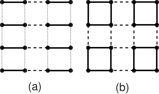
Figure 4: Sketch of the two simplest possible states with bond order for $S=1/2$ on the square lattice: (a) the columnar spin-Peierls states, and (b) plaquette state. The different values of $Q_{\bf a}({\bf r})$, defined in (17), on the links are encoded by the different line styles. Both states are 4-fold degenerate; an 8-fold degenerate state, with superposition of the above orders, also appears as a possible ground state of the generalized interface model.

A full analysis of the situation in $d=3$ has not been carried out. However, it is clear that a new state can appear in the phase diagram–the compact QED theory has a gapless Coulomb phase with a ‘photon’ excitation [47, 48, 49, 50]. In the quantum antiferromagnet, this photon corresponds to a collective spinless excitation with a gapless linear dispersion. It is likely that this Coulomb phase is insensitive to the Berry phases, has no bond order, and allows neutral $S=1/2$ spinon excitations. The analog of the bond-ordered states of $d=2$ should also be present.

Large scale numerical studies of $S=1/2$ quantum antiferromagnets on the square lattice which allow for the destruction of magnetic order in the ground state have only just become possible. Two studies have appeared recently [51, 52], and both present unambiguous evidence of bond order as shown in Fig 4.

3.1.2 Mobile charge carriers

The fate of the $d=2$ bond-ordered paramagnet upon doping with mobile charge carriers has been investigated in a number of studies [4, 38, 53, 54, 55]. As stated earlier, the bond order survives for a finite range of doping concentrations. Moreover, the ground state also acquires $d$-wave-like superconducting order which co-exists with bond order, a state first predicted in Ref. [4]. Loosely speaking, this superconductivity can be understood as a consequence of the mobility of the singlet valence bonds in Fig 3: the mobile pairs of electrons behave as Cooper pairs, and their Bose-Einstein condensation leads to superconductivity. The configuration and period of the bond order can also evolve with increasing density of carriers [38, 53, 55], especially if the parameters are such that the physics of frustrated phase separation is important [56]. The reader is referred to Ref. [2] for a recent review of this work, along with implication for a number of recent experiments on the cuprate superconductors. These experiments include a possible observation in STM of a state with co-existing bond order and $d$-wave superconductivity [57, 58, 59, 55, 60].

3.2 Collective mode fractionalization

We now consider magnetically ordered and paramagnetic states with collinear spin correlations at wavevectors other than ${\bf K}=(\pi,\pi,\ldots)$. For these cases the field $e^{i\theta}$, in the decomposition $\Phi_{\alpha}=e^{i\theta}n_{\alpha}$ in (4), cannot be disposed at the outset, and needs to be retained as an additional degree of freedom. The physical significance of this additional field is readily apparent from a comparison of the definitions (2) and (17) of the magnetic order parameters; a factorization of the expectation values in (17) implies that there is contribution [61, 62]:

$$Q_{\bf a}({\bf r})=\mbox{Re}\left[e^{2i\theta}e^{i{\bf K}\cdot(2{\bf r}+{\bf a})}\right]+\ldots$$ (25)

where we have assumed, as in Section 3.1.1, that $n_{\alpha}$ has been rescaled so that $n_{\alpha}^{2}=1$. So a collinear magnetically ordered state at wavevector ${\bf K}$ automatically has co-existing bond order modulations at wavevector $2{\bf K}$, and $e^{2i\theta}$ is the bond order parameter.

We can now combine this observation with the results of Section 3.1.1 to obtain a simple, and quite general, theory of the loss of magnetic order for the values of ${\bf K}$ under consideration here. As bond order co-exists with magnetic order, it is natural consider the possibility that the loss of magnetic order occurs in a ‘background’ of bond order, and the latter is present on both sides of the transition. In other words, we consider a transition from a magnetically ordered state with $\langle\Phi_{\alpha}\rangle\neq 0$ (and so necessarily $\langle e^{2i\theta}\rangle\neq 0$), to a paramagnetic state with bond order which has $\langle\Phi_{\alpha}\rangle=0$ but still $\langle e^{2i\theta}\rangle\neq 0$. We can assume that the background bond order is quenched, and hence need only consider a theory of $n_{\alpha}$ fluctuations in this environment.

For insulating systems, this theory will have essentially the same structure as that in Section 3.1.1, with the difference that the coupling constants will now acquire a modulation induced by the background bond order. The Berry phases will again attempt to induce bond order in the regime with strong fluctuations of $n_{\alpha}$, but this may be a redundant effort–the bond order is already present in the underlying Hamiltonian for the spins. As long as the underlying bond order has an even number of spins per unit cell, the upshot is that we can safely neglect the Berry phases, and the theory is simply that of a $n_{\alpha}$ field undergoing a ‘quantum disordering’ transition in a partition function with positive weights and short-range interactions: the critical theory for this is the O(3) $\varphi^{4}$ field theory in 2+1 spacetime dimensions.

For systems with mobile charge carriers, we have to consider possible long-range couplings induced by other gapless excitations. These effects are quite strong and relevant in metals, but are relatively unimportant in the superconducting states considered in Section 3.1.2: superconductors have low energy fermionic excitations at only select points in the Brillouin zone, and these usually couple quite weakly to the critical spin fluctuations [53].

Having disposed of this simple possibility for the loss of collinear magnetic order, let us now explore more fully the possible phases that are allowed in a general interplay of collinear magnetic and bond order parameters. The list of possibilities is very large, but interplay with experiments should help narrow the range of possibilities [36, 63, 64]. As in Section 2.1 a global view of the phase diagram is obtained most easily by constructing an effective action for a $Z_{2}$ gauge theory. The gauge theory must now be formulated for an order parameter on the manifold $(S_{2}\times S_{1})/Z_{2}$, rather than $S_{3}/Z_{2}$, but the strategy is quite similar to that of Section 2.1. We take the physical field $\Phi_{\alpha}$, and split it apart into its $n_{\alpha}$ and $e^{i\theta}$ constituents; the overall sign for the constituents involves a $Z_{2}$ gauge choice which can be made differently at distinct points in spacetime. We can compensate for this ambiguity by introducing a $Z_{2}$ gauge field, $\sigma_{ij}$ (note that the physical interpretation of this $\sigma_{ij}$ is entirely different from that in Section 2.1), and so obtain the effective partition function [36]:

$$\mathcal{Z}_{\rm coll} = \int\prod_{j}d\theta_{j}dn_{j\alpha}\delta\left(n_{j\alpha}^{2}-1\right)\sum_{\{\sigma_{ij}=\pm 1\}}\exp\left(-\mathcal{S}_{\rm coll}\right)$$

$$\mathcal{S}_{\rm coll} = -J_{3}\sum_{\langle ij\rangle}\sigma_{ij}n_{i\alpha}n_{j\alpha}-J_{4}\sum_{\langle ij\rangle}\sigma_{ij}\cos(\theta_{i}-\theta_{j})-K\sum_{\Box}\prod_{\langle ij\rangle\in\Box}\sigma_{ij}.$$ (26)

For commensurate values of ${\bf K}$ there will be an additional on-site anisotropy field arising from $V_{\rm comm}$ in (8) $\sim-w\sum_{j}\cos(2p\theta_{j})$.

What is the interpretation of a $Z_{2}$ gauge flux now ? It locates the position of defects often called “stripe dislocations”, sketched in Fig 5.

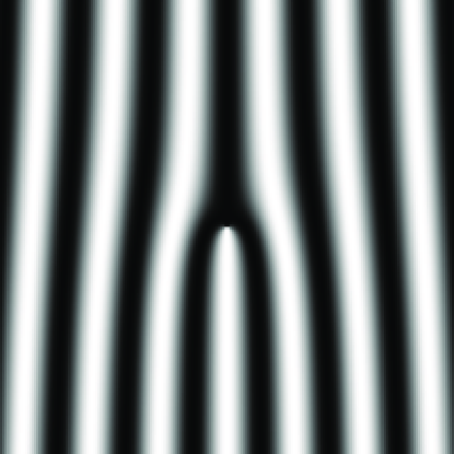
Figure 5: A stripe dislocation: gray scale plot of the bond order $Q_{\bf a}({\bf r})\sim\cos({\bf K}_{x}\cdot(2{\bf r}+{\bf a})+2\theta_{x})$ (see (25), (2) and (4)) with $\theta_{x}=\pi/2+(1/2)\tan^{-1}(y/x)$ containing a half vortex. The collective mode fractionalization transition is between phases with and without suppression of these defects. Both phases have neither magnetic or bond order.

To see this, consider, as in Section 2.1, the defects associated with $\pi_{1}((S_{2}\times S_{1})/Z_{2})$ [36]. These include ordinary vortices in the field $\theta$, under which $\theta$ winds by an integer multiple of $2\pi$ upon encircling the vortex. However, an additional class of half-vortices are also allowed for which the $Z_{2}$ quotient plays a crucial role: in these, $\theta$ winds by an half-odd-integer multiple of $2\pi$. At the same time, there is a corresponding trajectory for $n_{\alpha}$ which connects polar opposite points on $S_{2}$; this ensures that the physical field $\Phi_{\alpha}$ is single-valued everywhere. In the context of (26), we observe that, as in Section 2.1 and Fig 1, we will have $\sigma_{ij}=-1$ only between the initial and final points of the loop, to eliminate the branch cuts in $e^{i\theta}$ and $n_{\alpha}$. Hence each such half vortex carries a $Z_{2}$ gauge flux.

The phase diagram of $\mathcal{S}_{\rm coll}$ in the three-dimensional $J_{3,4},K$ space is quite complex, but many of its features can be understood by analyses of various two-dimensional sections, most of which bear some formal similarity to the model analyzed in Section 2.1. We do not want to run through the plethora of possibilities here, and will merely focus on a particular phase transition [63, 36] which has some intriguing experimental implications.

Consider the region of small $J_{3,4}$ where $\langle\Phi_{\alpha}\rangle=0$ and $\langle e^{2i\theta}\rangle=0$, and so there is no magnetic or bond order. Let us first take a small value of $K$—in the cuprates, we would imagine this is in the overdoped region; then the field $\sigma_{ij}$ will fluctuate strongly, and the stripe dislocations will proliferate. Such a state has no vestiges of either magnetic or bond order, and is therefore an ordinary superconductor or Fermi liquid. The strong $\sigma_{ij}$ fluctuations also ‘bind’ the $n_{\alpha}$ and $e^{i\theta}$ fields to each other in the $\Phi_{\alpha}$ field, and the latter constitutes a collective elementary excitation which carries both spin and bond correlations; indeed, $\Phi_{\alpha}$ is simply an ordinary collective particle-hole excitation which can be described by a time-dependent Hartree-Fock theory; in a superconductor, this excitation could also avoid damping from the particle-hole continuum, and so become a sharp quasiparticle. This collective mode has 6 real components, corresponding to the 3 complex numbers required to define $\Phi_{\alpha}$ [65].

Now increase the value of $K$; in the cuprates, this would correspond to moving towards the underdoped region. This will suppress the stripe dislocations until eventually there is a $Z_{2}$ gauge theory transition to a deconfined phase; this transition is the analog of the transition across the line MC in Fig 2. The deconfined phase has dislocations suppressed, and unbound quanta of $n_{\alpha}$ and $e^{i\theta}$. However it is still true that $\langle\Phi_{\alpha}\rangle=0$ and $\langle e^{2i\theta}\rangle=0$, and so there is no magnetic or bond order. So this is a fractionalized phase in which quanta of $\Phi_{\alpha}$ have separated into 3 real quanta of $n_{\alpha}$ and 2 real quanta of $e^{i\theta}$ i.e. the collective mode has fractionalized. Note that unlike the fractionalized phase of Section 2.1, there are no neutral $S=1/2$ excitations, and the electron always retains its bare quantum numbers.

Why is this $Z_{2}$ gauge fractionalization transition interesting ? First, unlike that in Section 2, it is based on correlations (collinear magnetic and bond) that are actually observed in the lightly doped cuprates. While long-range order with $\langle\Phi_{\alpha}\rangle\neq 0$ and $\langle e^{2i\theta}\rangle\neq 0$ is observed at low doping in some of the cuprates, it is quite clear that all such conventional order has essentially disappeared by the time we reach optimal doping. However, remnants of such order may still be present in that the stripe dislocations of Fig 5 have not yet proliferated. This then opens up the possibility [36, 63] of a quantum critical point near optimal doping [66, 67], associated with the proliferation of stripe dislocation with increasing doping, which is in the universality class of the 2+1 dimensional $Z_{2}$ gauge theory. As an added bonus, it has been recently argued [68] that this gauge theory remains strongly coupled even in the presence of Fermi surface damping, and so is an attractive candidate for anomalous behavior at higher temperatures.

4 Conclusions

This article has given a broad overview of phases of strongly interacting electrons, going beyond those found in the conventional Bloch-BCS theory of solid state physics. A plethora of exotic and conventional states have been proposed in the literature, and we attempted to bring some ‘order’ into the subject, by presenting a classification based on the physics of Mott insulators, and by making connections between the correlations in different states.

Some of the states considered here have conventional order parameters, and could, in principle, also be obtained from a weak-coupling instability of the Hartree-Fock/BCS theory of the Fermi liquid or superconductor. These include the states with collinear or non-collinear magnetic order, and with bond order. We have chosen here, instead, to motivate them from the states of the Mott insulator. Our approach properly accounts for the strongest energy scales at the outset (the local repulsion between nearby electrons), and so has a better handle on the energy scales of various excitations. The Hartree-Fock/BCS theory could obtain states with the same overall symmetry, but would give very different estimates of the relative stability and energies of various excitations. The selection of the wavevector, ${\bf K}$, would also be based upon the Fermi surface geometry. In contrast, the Mott-insulator-based approach used here, selects wavevectors from very different criteria: e.g. in the bond ordered states, it is the spin Berry phases and the resonance and alignment of singlet valence bonds which selects the state, and leads to predictions for the values of ${\bf K}$ [4, 38] which have little to do with the Fermi surface geormetry. These latter values appear to be consistent with observations [69].

Another value in starting with the Mott insulator is that it also allows a systematic classification of states with more exotic order parameters, which cannot be expressed in terms of local correlation functions. They appeared here as ‘quantum disordered’ states of different types of magnetic order; these ‘disordered’ states however possessed a topological order associated with the suppression of certain defects which were classified by the global topology of the magnetically ordered state. We also found a description of the dynamics of this topological order in two distinct $Z_{2}$ gauge theories, in systems with non-collinear and collinear spin correlations respectively.

With some understanding of global features of the phase diagram at hand, we can proceed with a study of possible quantum critical points, and their influence on crossovers at finite temperatures [39]. For the cuprates, these issues have been reviewed in Ref. [2]; the ‘stripe fractionalization’ transition of Section 3.2 is only poorly understood, and much additional work is required to understand its observable consequences. The most intensive investigation of quantum criticality has so far occurred in the heavy fermion compounds, and most observations do not agree with the weak-coupling spin density wave picture. Here, we think that the small Fermi surface state of Section 2.2.1 offers the prospect of leading to many interesting related states, and of non-trivial quantum critical points between them—this is an exciting avenue for further research.

Acknowledgements

I thank Eugene Demler, T. Senthil, and Matthias Vojta for recent collaborations upon which this review is based. This research was supported by US NSF Grant DMR 0098226.

References

- [1] D. J. Thouless, Topological Quantum Notes in Nonrelativistic Physics, World Scientific, Singapore, 1998.
- [2] S. Sachdev cond-mat/0211005.
- [3] N. Read, S. Sachdev, Phys. Rev. Lett. 66 (1991) 1773.
- [4] S. Sachdev, N. Read, Int. J. Mod. Phys. B 5 (1991) 219.
- [5] A. V. Chubukov, T. Senthil, S. Sachdev, Phys. Rev. Lett. 72 (1994) 2089.
- [6] A. V. Chubukov, T. Senthil, S. Sachdev, Nucl. Phys. B 426 (1994) 601.
- [7] T. Senthil, M. P. A. Fisher, Phys. Rev. B 62 (2000) 7850.
- [8] P. E. Lammert, D. S. Rokhsar, J. Toner, Phys. Rev. Lett. 70 (1993) 1650.
- [9] P. E. Lammert, D. S. Rokhsar, J. Toner, Phys. Rev. E. 52 (1995) 1778.
- [10] F. Wegner, J. Math. Phys. 12 (1971) 2259.
- [11] E. Fradkin, S. H. Shenker, Phys. Rev. D 19 (1979) 3682.
- [12] S. Sachdev, K. Park, Annals of Phys. 298 (2002) 58.
- [13] H. Kawamura, Phys. Rev. B 38 (1988) 4916.
- [14] A. Pelissetto, P. Rossi, E. Vicari, Phys. Rev. B 65 (2001) 020403.
- [15] A. Pelissetto, P. Rossi, E. Vicari, Nucl. Phys. B 607 (2001) 605.
- [16] P. Calabrese, P. Parruccini, A. I. Sokolov cond-mat/0205046.
- [17] P. Azaria, B. Delamotte, T. Jolicoeur, Phys. Rev. Lett. 64 (1990) 3175.
- [18] L. Pauling, Proc. Roy. Soc. London, A 196 (1949) 343.
- [19] P. Fazekas, P. W. Anderson, Philos. Mag. 30 (1974) 23.
- [20] P. W. Anderson, Science 235 (1987) 1196.
- [21] S. A. Kivelson, D. S. Rokhsar, J. P. Sethna, Phys. Rev. B 35 (1987) 8865.
- [22] X.-G. Wen, Phys. Rev. B 44 (1991) 2664.
- [23] R. Moessner, S. L. Sondhi, Phys. Rev. Lett. 86 (2001) 1881.
- [24] R. Coldea, D. A. Tennant, A. M. Tsvelik, Z. Tylczynski, Phys. Rev. Lett. 86 (2001) 1335.
- [25] R. Jalabert, S. Sachdev, Phys. Rev. B 44 (1991) 686.
- [26] S. Kivelson, Phys. Rev. B 39 (1989) 259.
- [27] N. Read, B. Chakraborty, Phys. Rev. B 40 (1989) 7133.
- [28] E. Demler, C. Nayak, H.-Y. Kee, Y.-B. Kim, T. Senthil, Phys. Rev. B 65 (2002) 155103.
- [29] S. Sachdev, Phys. Rev. B 45 (1992) 389.
- [30] N. Nagaosa, P. A. Lee, Phys. Rev. B 45 (1992) 966.
- [31] T. Senthil, M. P. A. Fisher, Phys. Rev. Lett. 86 (2001) 292.
- [32] J. C. Wynn, D. A. Bonn, B. W. Gardner, Y.-J. Lin, R. Liang, W. N. Hardy, J. R. Kirtley, K. A. Moler, Phys. Rev. Lett. 87 (2001) 197002.
- [33] D. A. Bonn, J. C. Wynn, B. W. Gardner, Y.-J. Lin, R. Liang, W. N. Hardy, J. R. Kirtley, K. A. Moler, Nature 414 (2001) 887.
- [34] T. Senthil, S. Sachdev, M. Vojta cond-mat/0209144.
- [35] S. Burdin, D. R. Grempel, A. Georges, Phys. Rev. B 66 (2002) 045111.
- [36] Y. Zhang, E. Demler, S. Sachdev, Phys. Rev. B 66 (2002) 094501.
- [37] N. Read, S. Sachdev, Phys. Rev. Lett. 62 (1989) 1694.
- [38] M. Vojta, S. Sachdev, Phys. Rev. Lett. 83 (1999) 3916.
- [39] S. Sachdev, Quantum Phase Transitions, Cambridge University Press, Cambridge, 1999.
- [40] S. Sachdev, Physica A 313 (2002) 252, cond-mat/0109419.
- [41] E. Fradkin, S. A. Kivelson, Mod. Phys. Lett. B 4 (1990) 225.
- [42] S. Sachdev, R. Jalabert, Mod. Phys. Lett. B 4 (1990) 1043.
- [43] A. D’Adda, P. D. Vecchia, M. Luscher, Nucl. Phys. B 146 (1978) 63.
- [44] E. Witten, Nucl. Phys. B 149 (1979) 285.
- [45] N. Read, S. Sachdev, Phys. Rev. B 42 (1990) 4568.
- [46] D. S. Rokhsar, S. A. Kivelson, Phys. Rev. Lett. 61 (1988) 2376.
- [47] T. Banks, J. Kogut, R. Myerson, Nucl. Phys. B 129 (1977) 493.
- [48] E. Fradkin, L. Susskind, Phys. Rev. D 17 (1978) 2637.
- [49] X.-G. Wen, Phys. Rev. Lett. 88 (2002) 011602.
- [50] O. I. Motrunich, T. Senthil cond-mat/0205170.
- [51] A. W. Sandvik, S. Daul, R. R. P. Singh, D. J. Scalapino, Phys. Rev. Lett. 89 (2002) 247201.
- [52] K. Harada, N. Kawashima, M. Troyer cond-mat/0210080.
- [53] M. Vojta, Y. Zhang, S. Sachdev, Phys. Rev. B 62 (2000) 6721.
- [54] K. Park, S. Sachdev, Phys. Rev. B 64 (2001) 184510.
- [55] M. Vojta, Phys. Rev. B 66 (2002) 104505.
- [56] V. J. Emery, S. A. Kivelson, H. Q. Lin, Phys. Rev. Lett. 64 (1990) 475.
- [57] C. Howald, H. Eisaki, N. Kaneko, A. Kapitulnik cond-mat/0201546.
- [58] C. Howald, H. Eisaki, N. Kaneko, M. Greven, A. Kapitulnik cond-mat/0208442.
- [59] D. Podolsky, E. Demler, K. Damle, B. I. Halperin cond-mat/0204011.
- [60] D. Zhang cond-mat/0210386.
- [61] O. Zachar, S. A. Kivelson, V. J. Emery, Phys. Rev. B 57 (1998) 1422.
- [62] A. Polkovnikov, S. Sachdev, M. Vojta, in: Proceedings of the 23rd International Conference on Low Temperature Physics, 2002, cond-mat/0208334.
- [63] J. Zaanen, O. Y. Osman, H. V. Kruis, Z. Nussinov, J. Tworzydlo, Phil. Mag. B 81 (2001) 1485.
- [64] J. Zaanen, Z. Nussinov cond-mat/0209441.
- [65] A. Polkovnikov, S. Sachdev, M. Vojta, E. Demler, in: G. Boebinger, Z. Fisk, L. P. Gor’kov, A. Lacerda, J. R. Schieffer (Eds.), Proceedings of Physical Phenomena at High Magnetic Fields-IV, World Scientific, Singapore, 2001, cond-mat/0110329.
- [66] T. Valla, A. V. Fedorov, P. D. Johnson, B. O. Wells, S. L. Hulbert, Q. Li, G. D. Gu, N. Koshizuka, Science 285 (1999) 2110.
- [67] J. L. Tallon, J. W. Loram, Physica C 349 (2001) 53.
- [68] S. Sachdev, T. Morinari cond-mat/0207167.
- [69] S. Sachdev cond-mat/0203363.