An optical fiber based interferometer to measure velocity profiles in sheared complex fluids

Abstract

We describe an optical fiber based interferometer to measure velocity profiles in sheared complex fluids using Dynamic Light Scattering (DLS). After a review of the theoretical problem of DLS under shear, a detailed description of the setup is given. We outline the various experimental difficulties induced by refraction when using a Couette cell. We also show that homodyne DLS is not well suited to measure quantitative velocity profiles in narrow-gap Couette geometries. On the other hand, the heterodyne technique allows us to determine the velocity field inside the gap of a Couette cell. All the technical features of the setup, namely its spatial resolution ($\approx 50$–$100~{}\mu$m) and its temporal resolution ($\approx 1$ s per point, $\approx 1$ min per profile) are discussed, as well as the calibration procedure with a Newtonian fluid. As briefly shown on oil-in-water emulsions, such a setup permits one to record both velocity profiles and rheological data simultaneously.

1 Introduction

The behaviour of complex fluids under flow raises important fundamental problems and involves a very wide spectrum of possible applications. A complex fluid is characterized by a mesoscopic scale, located somewhere between the microscopic size of the molecules and the macroscopic size of the sample Edimbourg:00 ; Larson:99 . For instance, for oil-in-water emulsions, this mesoscopic scale would be the size of an oil droplet. The existence of this mesoscopic scale can make the flow of a complex fluid considerably difficult to understand as compared to that of a simple, viscous fluid. Indeed, most of complex fluids show strong viscoelasticity and/or important nonlinear rheological behaviours.

These behaviours arise from coupling effects between the fluid microstructure and the flow. Usually, the presence of a shear flow tends to order the fluid, for instance, by aligning chains in a polymer solution and thus decreasing the viscosity (“shear thinning”). On the other hand, in a class of concentrated systems recently called “soft glassy materials”, such as concentrated emulsions or colloidal glasses, yield stress and jamming phenomena are frequently encountered Sollich:97 ; Viasnoff:02 .

Although the characterization of the global flow properties remains a first essential step, much interest has grown in performing local measurements on complex fluids under shear. Indeed, in many cases, inhomogeneous flows are observed for which the usual analysis in terms of pure shear flow is not applicable and may be misleading.

This paper is devoted to local velocimetry in sheared complex fluids using Dynamic Light Scattering (DLS). The need for local measurements is highlighted in the next Section through three examples taken from recent works in complex fluids. We then review a few existing techniques that provide local measurements and explain how they may or may not be suited to experiments in the concentric cylinder geometry (referred to as “Couette geometry” in the following). In Sec. 3, we give the basic theoretical principles of DLS under shear. In Sec. 4, we present an experimental setup based on the use of single mode optical fibers. Finally we show that the heterodyne geometry is better suited than the homodyne one when the fluid under study is sheared in a Couette cell.

2 The need for local measurements in the rheology of complex fluids

2.1 Examples of inhomogeneous flows in complex fluids

Complicated rheological behaviours are observed in complex fluids whose flow curves $\sigma(\dot{\gamma})$ are non-monotonic ($\sigma$ stands for the shear stress and $\dot{\gamma}$ for the shear rate). In such cases, above a critical shear rate, the stress may decrease resulting in a mechanical instability of the flow Spenley:93 . For controlled-shear-rate experiments, this type of instability is expected to show up on the flow curve as a stress plateau for $\dot{\gamma}_{1}<\dot{\gamma}\ <\dot{\gamma}_{2}$ separating two regions where the stress is an increasing function of the shear rate. Such a signature is indeed observed for various complex fluids such as wormlike micelle solutions Berret:97 or some lyotropic lamellar phases Roux:93 . On the stress plateau, the fluid is believed to phase-separate into two regions: one with high viscosity and low shear rate flowing at $\dot{\gamma}_{1}$ and one with low viscosity and high shear rate $\dot{\gamma}_{2}$. This phenomenon is known as shear banding. In micellar solutions, each “band” was shown to correspond to different fluid structures, isotropic or nematic, using flow birefringence Berret:97 or NMR spectroscopy Britton:97 . The correspondence between the branch flowing at $\dot{\gamma}_{2}$ and the nematic state is still under debate Fisher:01 .

Thus, even though the geometry and the nature of the deformation imposed on a complex fluid remain fairly simple (constant, homogeneous force or velocity at the wall of a Couette cell for instance), the response of the fluid may be highly nonlinear and sometimes spatially inhomogeneous. In some extreme cases, one not only observes bands of different structures and flow properties, but also large temporal fluctuations of the global sample viscosity Wunenburger:01 ; Bandyopadhyay:01 ; Salmon:02 . This last behaviour, recently coined “rheochaos” Cates:02 , is observed in the vicinity of the shear-induced transitions described above. The occurence of such dynamical behaviours shows that inhomogeneous flows of complex fluids can exist both spatially and temporally under simple shear, even in the absence of strong inertial or elastic effects Muller:89 ; Groisman:00 .

A simpler but recurrent problem in rheology is caused by wall slip. Unlike simple fluids, mixtures under shear may involve thin lubricating layers of low-viscosity fluid in the vicinity of the cell walls. These lubricating films absorb most of the viscous dissipation so that the fluid in the bulk is submitted to a shear rate smaller than that imposed globally. In emulsions, it is generally believed that apparent slip is due to “wall depletion”, the fluid close to the walls containing less oil droplets than in the bulk Barnes:95 . In classical rheology, wall slip is usually investigated by varying the cell characteristics and/or the wall rugosity Larson:99 . In any case, it remains a problem of considerable importance for industrial applications and shows yet another occurence of inhomogeneous flows in simple shear geometries.

2.2 Experimental constraints in the Couette geometry

Through the three examples of shear-banding, “rheochaos,” and wall slip, it clearly appears that local measurements are crucial to understand the physics underlying the response of many complex fluids to deformation and flow. However, most of the studies in this area still heavily rely on global data recorded by standard rheometers imposing a torque (a velocity resp.) on the axis of a moving cylindrical or conical part and measuring its velocity (the torque resp.) once the fluid is set into motion.

For more than two decades, great experimental effort has been devoted to developping new methods for measuring local quantities of rheological interest such as the local stress, the velocity field, or the local velocity gradient Britton:97 ; Fisher:01 ; Sanyal:00_1 ; Welch:02 . Ideally, such a technique should be implemented on standard rheometers. On these apparatus, various geometries are used to induce a pure shear flow: (i) Couette cells in which the fluid is confined in the gap $e$ between two coaxial cylinders and where the shear rate can be considered as homogeneous, provided the ratio of the gap to the cylinder radii $e/R$ is not too large, (ii) cone-and-plate cells which provide the best approximation of pure homogeneous shear flows, and (iii) plate-and-plate cells where the shear rate increases linearly with the radial position.

In the present paper, we will restrict ourselves to shear flows generated in a Couette cell. This particular geometry imposes a few important constraints:

1. The measurement technique has to be non intrusive. Indeed, the very high sensitivity of the material to local deformations precludes the use of a probe, such as the hot wires or the hot films classically used in hydrodynamics to record fluid velocities.

2. The thickness $e=1$–3 mm and the optical properties of the samples under investigation usually hinders direct optical access needed for techniques like Laser Doppler Velocimetry (LDV) or Fluorescence Correlation Spectroscopy (FCS): most complex fluids are not transparent and strongly scatter light. Also, in general, we are not able to directly follow individual droplets in an emulsion or fluorescent seeding particles in a lamellar phase. Let us point out, however, that direct tracking of the system is possible in the particular case of two-dimensional foams Debregeas:01 or when the fluid is transparent enough to allow Particle Imaging Velocimetry (PIV) measurements such as those by Pine et al. in Ref. Edimbourg:00 .

3. Finally, the curved geometry of a Couette cell induces refraction effects that can be relatively strong and make optical techniques relying on light scattering tricky to implement.

Moreover, a reliable measurement method should yield accurate, reproducible measurements with good temporal and spatial resolutions. Here, we shall call “good” a spatial resolution which provides, say, 20 measurement points accross the gap of our Couette cell, which is typically $e=1$–3 mm wide. Any technique that is able to distinguish volumes of fluid separated by 100 $\mu$m and measure their respective velocities (or any other local quantity) will thus have a good resolution.

2.3 NMR and DLS, two local measurements techniques

Among the few quantitative local techniques that have proved successful for complex fluids under flow are (i) Nuclear Magnetic Resonance (NMR) and (ii) Dynamic Light Scattering (DLS).

2.3.1 Nuclear Magnetic Resonance

Callaghan et al. have used NMR to image the velocity field of sheared wormlike micelles in both cone-and-plate and Couette ($e=1$ mm) geometries Britton:97 ; Fisher:01 . Results in the isotropic-nematic coexistence regime show a strong correlation between shear bands and bands of different structural order. NMR can resolve details down to 20 $\mu$m Britton:97 ; Fisher:01 and appears as a very powerful tool for local measurements in complex fluids. However, the main drawback of this technique is its poor temporal resolution: in Ref. Fisher:01 the authors report on a broad velocity distribution due to fluctuations of the flow field but are not able to resolve these fluctuations in time. Indeed, the accumulation time needed for one profile is about an hour.

Moreover, this technique requires the costly production and use of strong magnetic fields. Also, the flow cells have to be made nonmagnetic. This leads to even more important constraints on the design of the experiment.

2.3.2 Dynamic Light Scattering

Although subject to restrictions (2) and (3) listed above, DLS is a low-cost technique easier to set up, at least in the homodyne geometry. In the present work, these two restrictions can be partially avoided by controlling the optical index of the complex fluid under study. For instance by matching the indices of the aqueous phase and of the oil phase in an emulsion, we are able to control the amount of scattered light and avoid multiple scattering Salmon:02_3

DLS is a common tool for probing spatio-temporal correlations of the fluctuations of the dielectric permittivity in a material Berne:95 . With a realistic model of these fluctuations, DLS allows one to obtain information on the dynamics of the fluctuations at length scale $\lambda$, the wavelength of incident light. Such fluctuations may arise from different microscopic origins: if scattering particles are subject to Brownian motion then DLS yields a measurement of the diffusion coefficient of these particles Berne:95 ; in lyotropic lamellar systems, fluctuations arise from undulating membranes and DLS may be a useful tool to characterize the elasticity of the surfactant bilayers Nallet:88 .

In the simple case of a shear flow, it has been shown that homodyne DLS may give information on the local shear rate. Such a technique has been used to measure shear rate profiles of polymeric fluids in four-roll mill flows Sanyal:00_1 ; Wang:94 . However, this homodyne technique is not very well suited to the Couette geometry as we will see in the following. Ackerson and Clark Ackerson:81 have shown that heterodyne DLS was a powerful technique to measure local velocity and applied it to colloidal crystals under Couette flow. With the same kind of heterodyne setup, Gollub et al. studied velocity profiles in Newtonian fluids at the onset of the Taylor-Couette instability Gollub:74 ; Gollub:75 . In spite of the above results, very few local measurements using heterodyne DLS have been reported in the rheology literature. This is certainly due to the experimental difficulties to set up an interferometer around a Couette cell.

3 Theory of Dynamic Light Scattering in a shear flow

3.1 Homodyne and heterodyne DLS

The aim of this section is to give the basic theoretical principles of DLS under shear which are necessary to reduce the optical information to local shear rate and local velocity measurements. In a typical DLS experiment as sketched in Fig. 1, the sample is illuminated with coherent polarized laser light. Scattered light is collected at an angle $\theta$ by a photomultiplier tube $PMT$.

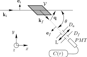
Figure 1: Geometry of homodyne DLS experiments. $PMT$ stands for photomultiplier tube. Other symbols are defined in the text.

The optical device which collects light is composed of a field diaphragm $D_{f}$ and a lens $L$. The scattering volume $\mathcal{V}$ is the intersection of the incident beam with the image of $D_{f}$ through $L$. The aperture diaphragm $D_{a}$ allows one to reduce the range of collected angles $\theta$ (it controls the size of the photodetection area). The auto-correlation function $C(\tau)=<\!i(t)i(t+\tau)\!>$ of the scattered intensity $i(t)$ is measured by an electronic correlator as a function of the time lag $\tau$. $\mathbf{e_{i}}$ is the direction of the polarization of the incident beam and $\mathbf{e_{f}}$ is the direction of the analyzer between the scattering volume and the $PMT$.

3.1.1 Homodyne DLS

When the dielectric permittivity tensor $\overline{\overline{\epsilon}}(\mathbf{r},t)$ of the material is slightly perturbated, i.e. when $\overline{\overline{\epsilon}}(\mathbf{r},t)=\epsilon\mathcal{I}+\overline{\overline{\delta\epsilon}}(\mathbf{r},t)$, and $\delta\epsilon\ll\epsilon$ ($\mathcal{I}$ is the unity tensor), the magnitude of the electric field scattered at angle $\theta$ is Berne:95 :

$$E_{s}(t)\propto\widehat{\delta\epsilon}_{if}(\mathbf{q},t)\,,$$

where $\mathbf{q}=\mathbf{k}_{i}-\mathbf{k}_{f}$ is the scattering vector, whose magnitude is given by $q=(4\pi n/\lambda)\sin(\theta/2)$, and $\widehat{\delta\epsilon}_{if}(\mathbf{q},t)$ is the $if$-component of the Fourier transform of the dielectric permittivity tensor of the sample restricted to the scattering volume $\mathcal{V}$:

$$\widehat{\delta\epsilon}_{if}(\mathbf{q},t)=\int_{\mathcal{V}}d^{3}\mathbf{r}e^{i\mathbf{q}\cdot\mathbf{r}}\mathbf{e_{i}}\overline{\overline{\delta\epsilon}}(\mathbf{r},t)\mathbf{e_{f}}\,.$$

In the following, we will focus on the $zz$-component of the tensor $\overline{\overline{\delta\epsilon}}(\mathbf{r},t)$, and we write for simplicity: $\delta\epsilon(\mathbf{r},t)=\delta\epsilon_{zz}(\mathbf{r},t)$.

Measuring the intensity scattered at angle $\theta$ allows one to determine the spatial fluctuations of the dielectric permittivity at length scale $q^{-1}$. In DLS, temporal fluctuations are studied through the correlation function $C(\tau)=<\!i(t)i(t+\tau)\!>$. If $\delta\epsilon(\mathbf{r},t)$ is a Gaussian random variable, one can show that Berne:95 :

$$C(\tau)=A+B|g^{(1)}(\tau)|^{2}\,,$$ (1)

where

$$g^{(1)}(\tau)=<\!\widehat{\delta\epsilon}(\mathbf{q},t)\,\widehat{\delta\epsilon}^{*}\!(\mathbf{q},t+\tau)\!>\,.$$

$A$ and $B$ are two constants that depend on the signal-to-noise ratio. $g^{(1)}(\tau)$ is the auto-correlation of the Fourier transform of the fluctuations of $\delta\epsilon(\mathbf{r},t)$ at length scale $q^{-1}$ and time $\tau$. A device measuring $|g^{(1)}(\tau)|^{2}$ is called a homodyne DLS setup.

3.1.2 Heterodyne DLS

In the case where the temporal fluctuations of $\delta\epsilon(\mathbf{r},t)$ are non-Gaussian or when $g^{(1)}(\tau)$ contains phase terms, homodyne DLS is not sufficient. To access the real part of $g^{(1)}(\tau)$, one has to use DLS in heterodyne mode. This method consists in measuring the signal resulting from the interference between the scattered electric field $\mathbf{E}_{s}$ and a local oscillator $\mathbf{E}_{\scriptscriptstyle LO}$ taken from the incident beam, whose magnitude is much greater than the scattered electric field. In this case, one can show that the autocorrelation function of $\mathbf{E}_{s}+\mathbf{E}_{\scriptscriptstyle LO}$ satisfies Berne:95 :

$$C(\tau)=A^{\prime}+B^{\prime}\mathcal{R}e\left(g^{(1)}(\tau)\right)\,,$$ (2)

where $A^{\prime}$ and $B^{\prime}$ are two constants that depend on the signal-to-noise ratio.

3.2 A simple model for $g^{(1)}(\tau)$ in a shear flow

3.2.1 Physical considerations

Let us now turn to the case when the scattering volume is submitted to a shear flow, as shown in Fig. 2. The theoretical problem of DLS in a shear flow has been extensively studied Wang:94 ; Ackerson:81 ; Fuller:80 ; Maloy:92 . The main result of these works is that homodyne DLS allows one to measure the local shear rate through decorrelation terms of geometrical nature.

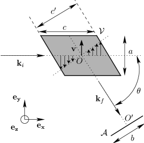
Figure 2: Geometry of the scattering volume in a shear flow. $\mathcal{V}$ stands for the scattering volume and $\mathcal{A}$ for the photocathode area.

On the other hand, heterodyne DLS yields an estimate of the mean velocity in the scattering volume using the well-known Doppler effect. Indeed, since scattering particles are moving at velocity $\mathbf{v}$, the frequency of the scattered electric field is Doppler shifted by the quantity $\mathbf{q}\!\cdot\!\mathbf{v}$. It is straightforward to show that $g^{(1)}(\tau)=F(\tau)\,\exp(i\mathbf{q}\!\cdot\!\mathbf{v}\tau)$, where $F(\tau)$ is some decreasing geometrical factor. Since homodyne DLS measures the modulus of $g^{(1)}(\tau)$, the local velocity can only be accessed by using the heterodyne configuration.

The aim of this section is to give some simple physical ideas that help to understand the correlation functions measured with heterodyne DLS. We then present more detailed equations which will be solved numerically in Sec. 4.

The geometry of DLS under shear is shown in Fig. 2. The incident beam is normal to the velocity ($y$) and to the vorticity ($z$) directions. In a shear flow, one expects the following invariance rule for the correlation of the fluctuations Ackerson:81 :

$$\Gamma(\mathbf{r},t,\mathbf{r^{\prime}},t^{\prime})\widehat{=} <\!\delta\epsilon(\mathbf{r},t)\delta\epsilon(\mathbf{r^{\prime}},t^{\prime})\!>$$

$$= \,\Gamma(\mathbf{r^{\prime}}-\mathbf{r}-(\mathbf{v}+\dot{\gamma}(\mathbf{r}.\mathbf{e}_{x})\mathbf{e}_{y})(t^{\prime}-t),t^{\prime}-t)\,.$$ (3)

Thus, in the presence of a shear flow, the physical properties in the scattering volume are no longer invariant under spatial translations. Hence the spatial coherence of the scattered electric field is modified Maloy:92 . From Eq. (3), one can show that:

$$<\!\widehat{\delta\epsilon}(\mathbf{q},t)\widehat{\delta\epsilon}(\mathbf{-q^{\prime}},t+\tau)\!>\neq 0\,,$$ (4)

only if the following condition is satisfied:

$$\mathbf{q^{\prime}}=\mathbf{q}+\dot{\gamma}\tau(\mathbf{q}.\mathbf{e}_{y})\mathbf{e}_{x}\,.$$ (5)

In fact, this relation is strictly true only for an infinite scattering volume. In practice, $\mathcal{V}$ corresponds to the intersection of two infinite cylinders. Therefore, the scattering volume has dimensions of the order of $a\times a\times c$ (cf. Fig. 2), and the scattering vectors $\mathbf{q}$ are only defined up to the precision $\delta q_{x}=\pm 2\pi/c$ and $\delta q_{y}=\delta q_{z}=\pm 2\pi/a$. Due to the finiteness of the scattering volume, light scattered at a distance $R$ corresponds to speckle grains and is spatially coherent in small coherence areas of typical size $\lambda R/c$. In the experiments, the aperture diaphragm $D_{a}$ collects a small range of angles $\theta$ and therefore a small range of $\mathbf{q}$’s. In this more realistic case, the correlation function measured with heterodyne DLS reads:

$$g^{(1)}(\tau)=\sum_{\mathbf{q},\mathbf{q^{\prime}}\in\mathcal{A}}<\!\widehat{\delta\epsilon}(\mathbf{q},t)\widehat{\delta\epsilon}(\mathbf{-q^{\prime}},t+\tau)\!>\,,$$ (6)

where the sum is calculated over the coherence areas which are collected on the $PMT$. In the presence of shear, due to the condition of Eq. (5), one can see that coherence areas are moving in the $x$-direction. This leads to decorrelation when $\|\mathbf{q^{\prime}}-\mathbf{q}\|>\delta q_{x}$ i.e. when $\tau>\tau_{\dot{\gamma}}=2\pi/(c\dot{\gamma}q_{y})$.

Another decorrelation time arises from the finiteness of the photocathode area. Indeed, speckle grains move out of the photodetection area due to the spatial coherence condition of Eq. (5). The separation $\delta R$ at a time $\tau$ between two coherence areas which contribute to $C(\tau)$ is of the order of $\delta R\approx\|\mathbf{q^{\prime}}-\mathbf{q}\|R/k_{f}\approx\dot{\gamma}R\tau$. Thus, for times $\tau>\tau_{\mathcal{A}}=b/(\dot{\gamma}R)$, this term leads to the decorrelation of $C(\tau)$ because the two coherence areas are separated by more than the characteristic length $b$ of the photocathode area.

Finally there is a third decorrelation time due to the transit time $\tau_{t}$ of the particles through the scattering volume $\mathcal{V}$. This transit time is of the order of $\tau_{t}\approx a/v$, where $v$ is the mean velocity in the scattering volume. In a lot of experimental situations however one has: $\tau_{t}\gg\tau_{\dot{\gamma}}$ and $\tau_{t}\gg\tau_{\mathcal{A}}$ so that this decorrelation cannot be observed. Physical systems may also display intrinsic dynamics such as Brownian motion. Such dynamics leads to decorrelation but in most systems the decorrelation times associated to those dynamics are very large compared to the geometrical times discussed above and cannot be observed Ackerson:81 .

From these physical considerations, we can assess that $g^{(1)}(\tau)$ takes the following form:

$$g^{(1)}(\tau)=e^{i\mathbf{q}\cdot\mathbf{v}\tau}F(\tau_{\mathcal{A}},\tau_{\dot{\gamma}},\tau)$$ (7)

3.2.2 Derivation of $F(\tau_{\mathcal{A}},\tau_{\dot{\gamma}},\tau)$

We now present a detailed derivation of the heterodyne correlation function under shear. In order to estimate $C(\tau)$ in realistic conditions, one must take into account the finiteness of the scattering volume $\mathcal{V}$ and of the photocathode area $\mathcal{A}$ as sketched in Fig. 3.

Figure 3: Typical configuration for light scattering in realistic conditions. $\mathcal{V}$ is the scattering volume, $\mathcal{A}$ the photocathode area

One can show that the magnitude of the electric field scattered at point $\mathbf{R}=\mathbf{R_{\scriptscriptstyle 0}}+\mathbf{r^{\prime}}$ from the scattering volume $\mathcal{V}$ is given by Berne:95 :

$$E_{s}(\mathbf{R},t)=\frac{k_{f}^{2}E_{\scriptscriptstyle 0}e^{i(k_{i}R_{\scriptscriptstyle 0}-\omega t)}}{4\pi\epsilon_{\scriptscriptstyle 0}R_{\scriptscriptstyle 0}}e^{i\mathbf{k}_{f}.\mathbf{r^{\prime}}}\widehat{\delta\epsilon}\left(\mathbf{q}+\frac{k_{f}}{R_{\scriptscriptstyle 0}}\mathbf{r^{\prime}},t\right)\,,$$ (8)

with $\mathbf{q}=\mathbf{k}_{f}-\mathbf{k}_{i}$ and assuming that $R\gg r$ and $R\gg r^{\prime}$. $R_{\scriptscriptstyle 0}$ is the distance between the center $O^{\prime}$ of the photocathode area $\mathcal{A}$ and the center $O$ of the scattering volume $\mathcal{V}$.

In heterodyne DLS, the normalized correlation function takes the following form:

$$C(\tau)\propto\mathcal{R}e\left(\iint_{\mathcal{A}}<\!E_{s}(\mathbf{R^{\prime}},t)E_{s}^{*}(\mathbf{R^{\prime\prime}},t+\tau)\!>\right)\,.$$ (9)

Using Eq. (8), one gets:

$$C(\tau)\propto\mathcal{R}e \iint_{\mathcal{A}}d\mathbf{r^{\prime}}d\mathbf{r^{\prime\prime}}e^{i\mathbf{k}_{f}\cdot(\mathbf{r^{\prime}}-\mathbf{r^{\prime\prime}})}$$

$$\left<\!\widehat{\delta\epsilon}\left(\mathbf{q}+\frac{k_{f}}{R_{\scriptscriptstyle 0}}\mathbf{r^{\prime}},t\right)\widehat{\delta\epsilon}^{*}\left(\mathbf{q}+\frac{k_{f}}{R_{\scriptscriptstyle 0}}\mathbf{r^{\prime\prime}},t+\tau\right)\!\right>\,.$$ (10)

Including the effect of shear requires a model for the dielectric permittivity of the material. A simple approach consists in considering isotropic, independent, point-like scatterers moving in a shear flow. In such a case, $\delta\epsilon(\mathbf{r},t)=\sum_{i=1}^{N}\delta(\mathbf{r}-\mathbf{r_{i}}(t))$ and $\mathbf{r_{i}}(t+\tau)=\mathbf{r_{i}}(t)+\mathbf{v}\tau+\dot{\gamma}x\mathbf{e}_{y}\tau$ (see Fig. 2). Eq. (10) can then be rewritten as :

$$C(\tau)\propto\mathcal{R}e \iint_{\mathcal{A}}d\mathbf{r^{\prime}}d\mathbf{r^{\prime\prime}}e^{i\mathbf{k}_{f}\cdot(\mathbf{r^{\prime}}-\mathbf{r^{\prime\prime}})}$$

$$\int_{\mathcal{V}}d\mathbf{r}\,e^{i\mathbf{q}\cdot(\mathbf{v}+\dot{\gamma}x\mathbf{e}_{y})\tau}e^{i(k_{f}/R_{\scriptscriptstyle 0})[\mathbf{r}\cdot(\mathbf{r^{\prime}}-\mathbf{r^{\prime\prime}})+\mathbf{r^{\prime}}\cdot(\mathbf{v}+\dot{\gamma}x\mathbf{e}_{y})\tau]}\,.$$ (11)

To proceed further in the discussion, the shape of the scattering volume and of the photocathode area have to be specified, so that Eq. (11) can be solved numerically.

4 DLS experiments in a Couette flow

4.1 Description of the experimental device

As discussed in the Introduction, one of the major challenges in the study of complex fluid flows is to measure simultaneoulsly the global rheology of a material under shear and the velocity profile inside the fluid. In order to perform such experiments we have developed the setup sketched in Fig. 4, where heterodyne DLS has been installed around a classical rheometer (TA Instruments AR 1000).

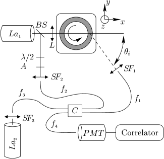
Figure 4: Heterodyne DLS setup. $La$ denotes lasers, $BS$ a beam splitter, $SF$ spatial filters, and $C$ the device coupling optical fibers $f$

In order to probe the rheological properties of our complex fluids, we use a transparent Mooney-Couette cell whose geometrical characteristics are given in the next paragraph. The temperature of the sample is controlled within $\pm\,0.1^{\circ}$C using a water circulation around the cell. The rheometer sits on a mechanical table whose displacements are controlled by a computer. Three mechanical actuators allow us to move the rheometer in the $x$, $y$, and $z$ directions with a precision of $1~{}\mu$m.

A $He$-$Ne$ polarized laser beam $La_{\scriptscriptstyle 1}$ ($40$ mW, $\lambda=632.8$ nm) is directed through the cell and is focussed inside the gap by a lens $L$ ($f=10$ cm). The incident beam is polarized along the $z$ direction. A spatial filter $SF_{\scriptscriptstyle 1}$, composed of a microscope lens and a single mode optical fiber $f_{\scriptscriptstyle 1}$ (core diameter $d=4~{}\mu$m, IDIL) collects the electric field scattered at an imposed angle $\theta_{i}$ by the sample lying in the gap.

In order to perform heterodyne measurements, a local oscillator is obtained from the incident beam by a beam splitter $BS$ and a second spatial filter $SF_{\scriptscriptstyle 2}$ which directs light into single mode fiber $f_{\scriptscriptstyle 2}$. The interference between this local oscillator and the scattered electric field is achieved by a single mode coupling device $C$ which connects fibers $f_{\scriptscriptstyle 1}$ and $f_{\scriptscriptstyle 2}$. This allows for great flexibility when choosing the scattering angle. From the output of $C$, the electric field arising from the interference propagates through single mode fiber $f_{\scriptscriptstyle 4}$ to a photomultiplier tube $PMT$ (Thorn EMI Type 9868), which is connected to an electronic correlator (Malvern Series 7032 with 64 channels).

Between $SF_{\scriptscriptstyle 2}$ and beam splitter $BS$, an attenuator $A$ avoids a too high illumination of the photomultiplier tube. A retardation plate ($\lambda/2$ plate) permits us to change the polarization of the light entering $f_{\scriptscriptstyle 2}$. The axis of the $\lambda/2$ plate is tuned in such a way that the two electric fields entering $C$ have the same polarization. Thus, the interference between the scattered electric field and the local oscillator measured with the $PMT$ is optimal.

To access the geometrical features of the scattering volume $\mathcal{V}$, we can turn on a second laser $La_{\scriptscriptstyle 2}$ ($He$-$Ne$, $10$ mW), which is coupled to single mode fiber $f_{\scriptscriptstyle 3}$ via spatial filter $SF_{\scriptscriptstyle 3}$. Light from $La_{\scriptscriptstyle 2}$ propagates through $f_{\scriptscriptstyle 3}$, then through $f_{\scriptscriptstyle 1}$ and goes out via $SF_{\scriptscriptstyle 1}$. Therefore we get a direct visualization of the scattering volume $\mathcal{V}$ as the intersection of the incident beam with the beam from $La_{\scriptscriptstyle 2}$.

4.2 Design of the Couette cell and refraction effects

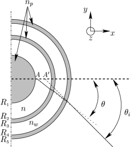
Figure 5: Experimental Couette cell. Plexiglas (optical index $n_{p}$) is indicated in gray. The sample (optical index $n$) lies between $R_{\scriptscriptstyle 1}$ and $R_{\scriptscriptstyle 2}$ and the thermostated water (optical index $n_{w}$) between $R_{\scriptscriptstyle 3}$ and $R_{\scriptscriptstyle 4}$.

In the experimental setup described in Sec. 4.1, one of the major constraints is the use of a thermostated Couette cell. Indeed, our home-made cell sketched in Fig. 5 is composed of four cylindrical interfaces. These interfaces separate the fluid under study from the water used for temperature control. This Couette cell thus acts as a cylindrical lens which leads to various optical complications: (i) the angle $\theta_{i}$ imposed by the operator differs from the actual scattering angle $\theta$, and (ii) the scattering volume lies at point $A$ instead of point $A^{\prime}$ (see Fig. 5). This leads to intricacies in the experimental determination of the positions of the stator and the rotor. Moreover when the Couette cell is moved in the $x$ direction by a quantity $\delta x$, the real displacement $\delta x^{\prime}$ of the scattering volume slightly differs from $\delta x$.

All these problems due to refraction must be taken into account in order to get reliable velocity profiles. To explicit the different relationships between $\theta$, $\theta_{i}$, $\delta x$, and $\delta x^{\prime}$, we simply write the Snell-Descartes laws for the four interfaces. The geometrical parameters are as follows: $R_{\scriptscriptstyle 1}=22,R_{\scriptscriptstyle 2}=25,R_{\scriptscriptstyle 3}=27.6,R_{\scriptscriptstyle 4}=30.5$ and $R_{\scriptscriptstyle 5}=35.6$ mm. Hence, the aspect ratio of our Couette cell is: $(R_{\scriptscriptstyle 2}-R_{\scriptscriptstyle 1})/R_{\scriptscriptstyle 2}=0.12$. All the fluids studied in this paper have the same optical index $n=1.40$. The optical indices of Plexiglas and water are $n_{p}=1.47$ and $n_{w}=1.33$ respectively. The imposed angle is $\theta_{i}=35^{\circ}$. With such parameters, Snell-Descartes laws lead to $\delta x^{\prime}=f_{x}\delta x$ with $f_{x}\approx 1.13$ and $\theta=f_{\theta}\theta_{i}$ with $f_{\theta}\approx 0.79$. We checked that $f_{x}$ does not depend on the position in the gap up to a very good approximation. However $\theta$ depends slightly on $x$ via $f_{\theta}$: its relative variation is $\delta\theta/\theta\approx 3~{}\%$ across the cell gap.

This last point is very important because the experimentally measured quantity, the Doppler shift $\mathbf{q}\!\cdot\!\mathbf{v}$, depends on the scattering angle. When scanning the width of the gap during an experiment, this small variation of $\theta$ leads to the following intrinsic incertitude on the velocity $\mathbf{v}$: $\delta v/v\approx 3~{}\%$. Let us notice however that this uncertainty strongly depends on the gap width: in a narrower gap, for instance $e=1$ mm, $\delta v/v\approx 1~{}\%$.

In the next paragraph we show that the use of single mode fibers leads to a simplification of Eq. (11) and we present measurements of the shape of the scattering volume using laser $La_{\scriptscriptstyle 2}$. Such measurements will allow us to compute the theoretical correlation function.

4.3 Numerical derivation of the heterodyne correlation function under shear

4.3.1 A simplification due to single mode fibers

A single mode fiber intrinsically collects coherent light only. Therefore the number of coherence areas detected by single mode fiber $f_{\scriptscriptstyle 1}$ is one: the size of the photocathode area does not play any role in our case. This feature is consistent with the experimental results presented in Sec. 4.4.1 where we will stress the fact that the only relevant geometrical time is $\tau_{\dot{\gamma}}$. According to this simplification, Eq. (11) can be rewritten as:

$$C(\tau) \propto\cos(\mathbf{q}\!\cdot\!\mathbf{v})\int_{\mathcal{V}}e^{i\dot{\gamma}xq_{y}\tau}\,.$$ (12)

To proceed further in the integration of Eq. (12), one has to know the exact shape of the scattering volume.

4.3.2 Shape of the scattering volume

The geometry of the scattering volume depends on the field diaphragm $D_{f}$, the focal length of the lens used in spatial filter $SF_{\scriptscriptstyle 1}$ and the distance $R$ between $SF_{\scriptscriptstyle 1}$ and the scattering volume $\mathcal{V}$.

To determine the size of $\mathcal{V}$, we image $\mathcal{V}$ using laser $La_{2}$ as explained in Sec. 4.1. With a sharp blade moving across the beam and perpendicular to the beam, we measured the transmitted intensity for different heights $z$ of the blade (see Fig. 6(a)).

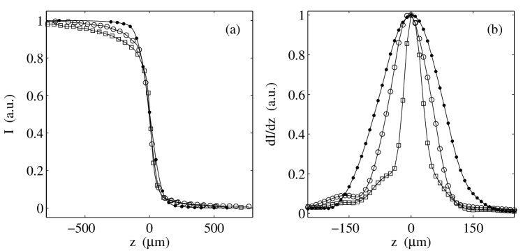
Figure 6: (a) Intensity collected on a photodiode by moving a sharp blade across the beam collecting the scattered light and visualized by turning on laser La₂ (see Fig. 4). (b) Intensity profile across the beam collecting the scattered light. The focal length of the microscope lens of spatial filter $SF_{\scriptscriptstyle 1}$ is 2.9 mm ($\bullet$), 5.5 mm ($\circ$), and 11 mm ($\Box$).

From this measurement, the intensity profiles of the beam are easily obtained by differentiating the previous signals (see Fig. 6(b)). In Fig. 6, the focal length of spatial filter $SF_{\scriptscriptstyle 1}$ was varied and the intensity profiles were measured at the distance $R=13$ cm from $SF_{\scriptscriptstyle 1}$ after the image of single mode fiber $f_{\scriptscriptstyle 1}$ was focussed on the blade (see below). Such a method allows us to estimate the typical size $c^{\prime}$ of the scattering volume. We chose to define $c^{\prime}$ as the half-width of the intensity profiles at the relative intensity $I/I_{\scriptscriptstyle 0}=e^{-2}$. As shown in Fig. 6(b), the minimum size is obtained for the focal length $f=11$ mm: $c^{\prime}\approx 40~{}\mu$m. This is consistent with the geometrical magnification factor $\gamma\approx R/f\approx 10$ which yields $c^{\prime}\approx\gamma d\approx 40~{}\mu$m, where $d=4~{}\mu$m is the core diameter of the fiber and $R=13$ cm.

To make sure that the image of single mode fiber $f_{\scriptscriptstyle 1}$ is located exactly on the blade, one has to measure the width of the beam at the position of the blade for different defocusing distances $d_{\scriptscriptstyle FL}$ between the lens and single mode fiber $f_{\scriptscriptstyle 1}$. In Fig. 7, we plotted the characteristic length $c^{\prime}$ measured for different distances $d_{\scriptscriptstyle FL}$ with the lens of focal length $f=11$ mm. This curve shows a minimum at the distance $d_{\scriptscriptstyle FL}$ for which the image of the single mode fiber by the lens lies exactly on the blade. This yields the typical characteristic length $c^{\prime}=40~{}\mu$m reported above in Fig. 6(b). When the refraction effects induced by the Couette cell are taken into account, the length $c$ displayed in Fig. 2 is given by $c=f_{x}c^{\prime}/\sin(f_{\theta}\theta_{i})\approx 100~{}\mu$m.

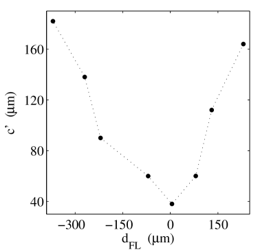
Figure 7: Width of the scattering volume $c^{\prime}$ measured from the intensity profiles for different “defocusing” distances $d_{\scriptscriptstyle FL}.$ The focal length of $SF_{\scriptscriptstyle 1}$ is 11 mm.

Using the same method with laser $La_{\scriptscriptstyle 1}$, we obtained the transverse dimension $a$ of the scattering volume: $a\approx 20~{}\mu$m. This characteristic size is consistent with the relation for Gaussian beams: $a\approx\lambda f/(\pi\omega_{\scriptscriptstyle{0}})\approx 20~{}\mu$m where $\omega_{\scriptscriptstyle{0}}\approx 1$ mm is the beam waist of the incident light and $f=10$ cm is the focal length of lens $L$.

4.3.3 Numerical integration of $C(\tau)$

We computed $C(\tau)$ from Eq. (12) using the experimental profile for the scattering volume and with a space dilation factor $f_{x}/\sin\theta$ due to the Couette cell. This leads to the results displayed in Fig. 8. In Fig. 8(a) is shown the square of heterodyne correlation functions calculated from Eq. (12) with $v=0$ for various shear rates. These functions are thus equal to $|g^{(1)}(\tau)|^{2}$ and are also exactly equal to the normalized homodyne correlation functions (see Eq. (7)). In Fig. 8(b), we plotted the half-time $\tau_{\scriptscriptstyle{1/2}}$ of the computed homodyne functions, defined by $C(\tau_{\scriptscriptstyle{1/2}})=1/2$, vs. various shear rates. All the qualitative features of homodyne DLS under shear are reproduced by Eq. (12). For instance, the continuous line in Fig. 8(b) shows that $\tau_{\scriptscriptstyle{1/2}}\propto\dot{\gamma}^{-1}$, as expected from the physical ideas discussed above.

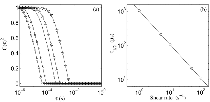
Figure 8: (a) Theoretical homodyne correlation functions computed from Eq. (12) with $v=0$ for various shear rates $\dot{\gamma}=1$ s${}^{-1}~{}(\triangledown)$, 5 s${}^{-1}~{}(\triangle)$, 10 s${}^{-1}~{}(+)$, 50 s${}^{-1}~{}(\times)$ and 100 s${}^{-1}~{}(\circ)$. (b) Computed $\tau_{\scriptscriptstyle{1/2}}$ vs. shear rate. The solid line is the best fit by a power law: $\tau_{\scriptscriptstyle{1/2}}\propto\dot{\gamma}^{-0.99}$

4.4 Calibration of the experiment using a Newtonian fluid

To proceed further, one has to perform calibration experiments with a well-known flow. We used a dilute suspension of latex spheres ($\phi\approx 0.1~{}\%$ wt.) in a 1:1 water-glycerol mixture. The optical index of the suspension was measured to be $n=1.40\pm 0.01$. The imposed scattering angle is $\theta_{i}=35^{\circ}$. This mixture is a Newtonian solution and, in a Couette cell of aspect ratio $e/R_{\scriptscriptstyle 2}=0.12$, we expect to measure velocity profiles that are very close to straight lines. In the following, we present experimental data showing that, even if in principle the homodyne geometry allows us to estimate the local shear rate, it is not a suitable method to measure velocity profiles in a Couette cell because of the strong influence of the shape of the scattering volume and because of the uncertainties on the exact positions of the rotor and the stator. On the other hand, we show that the heterodyne geometry is a time- and space-resolved method to perform local velocimetry.

Typical normalized correlation functions obtained under shear ($\dot{\gamma}=10$ s^-1) are presented in Fig. 9 where the square root of the homodyne function is plotted in order to be compared to the heterodyne one. As expected from Eqs. (1) and (7), $C(\tau)^{1/2}$ in homodyne mode corresponds to the envelope of the oscillating heterodyne function. Moreover this envelope shows a strong decorrelation at time $\tau\approx 80~{}\mu$s.

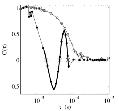
Figure 9: Experimental homodyne ($\circ$) and heterodyne ($\bullet$) correlation functions recorded on a latex suspension under shear at $\dot{\gamma}=10$ s^-1. The measurements were taken at $x_{t}=14.60$ mm i.e. 1.20 mm away from the moving inner wall. The thick line shows the portion of the heterodyne function that is used in the data analysis to determine the zero crossings ($\times$) from which the local velocity is calculated (see text).

4.4.1 Experimental features of homodyne DLS under shear

Let us first consider homodyne correlation functions. In Fig. 10, the half-time $\tau_{\scriptscriptstyle{1/2}}$ of homodyne correlation functions is plotted against the imposed shear rate $\dot{\gamma}$. This time scales as $\tau_{\scriptscriptstyle{1/2}}\propto\dot{\gamma}^{-1}$. Since the characteristic geometrical times scale as $\tau_{\dot{\gamma}}\propto\dot{\gamma}^{-1}$ and $\tau_{\mathcal{A}}\propto\dot{\gamma}^{-1}$, this is the scaling expected from theory. Moreover the measured $\tau_{\scriptscriptstyle{1/2}}(\dot{\gamma})$ are in good agreement with those computed from Eq. (12) and displayed in Fig. 8(b).

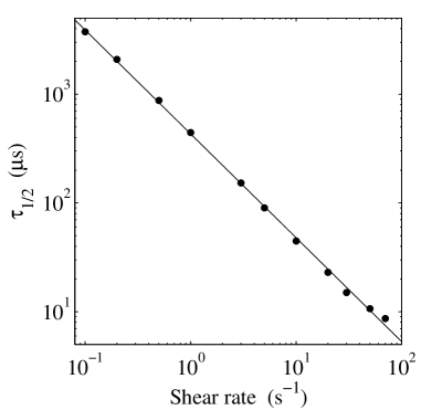
Figure 10: Half-time $\tau_{\scriptscriptstyle{1/2}}$ of the homodyne correlation function measured in the middle of the gap for $d_{FL}=200~{}\mu$m vs. shear rate. For each data point, the correlation function was accumulated over 1 min. The solid line is a power-law fit with exponent -0.99.

In Fig. 11, we plotted $\tau_{\scriptscriptstyle{1/2}}$ for different defocusing distances $d_{\scriptscriptstyle FL}$ at a given shear rate $\dot{\gamma}=10$ s^-1. As explained above, changing the distance $d_{\scriptscriptstyle FL}$ between the lens and the single mode fiber increases the width of the beam at a fixed distance $R$. Therefore one expects an increase of the size of the scattering volume $\mathcal{V}$. As shown in Fig. 11, this leads to a decrease of the characteristic time $\tau_{\scriptscriptstyle{1/2}}$. This behaviour can be expected from theory if one considers $\tau_{\dot{\gamma}}\propto(c\dot{\gamma})^{-1}$. From these results, it seems that the relevant time which governs the correlation function $C(\tau)$ is $\tau_{\dot{\gamma}}$. It is in agreement with the features discussed in Sec. 4.3, where we emphasized that $\tau_{\mathcal{A}}$ should not play any significant role thanks to the use of single mode fibers.

Figure 11: Half-time $\tau_{\scriptscriptstyle{1/2}}$ of the homodyne correlation function measured in the middle of the gap at $\dot{\gamma}=10$ s^-1 vs. “defocusing” distance $d_{FL}$. For each data point, two correlation functions were accumulated over 1 min and the two values of $\tau_{\scriptscriptstyle{1/2}}$ were averaged. The error bars account for the difference between those two estimates.

Homodyne DLS allows quantitative measurements of the local shear rate only if the shape of the scattering volume $\mathcal{V}$ is precisely known. In our experiment, the scattering volume is obviously not well defined mainly because of the refraction effects induced by the Couette cell. For instance a small motion the Couette cell can change the shape of the scattering volume.

In Fig. 12, we plotted the half-time $\tau_{\scriptscriptstyle{1/2}}$ of homodyne correlation functions for various positions $x_{t}$ of the mechanical table and for two different defocusing distances $d_{\scriptscriptstyle FL}$. For $d_{\scriptscriptstyle FL}=0$, the values of $\tau_{\scriptscriptstyle{1/2}}$ show a dispersion of about $20~{}\%$ and for $d_{\scriptscriptstyle FL}=200~{}\mu$m, the dispersion is about $50~{}\%$. In both cases the half-times significantly grow when approaching the two walls. This effect, which accounts for most of the observed dispersion, is due to the fact that the size of scattering volume decreases when $\mathcal{V}$ intersects one of the cell walls. This increase of $\tau_{\scriptscriptstyle{1/2}}$ is particularly noticeable when $d_{\scriptscriptstyle FL}=200~{}\mu$m because in this case the scattering volume is about twice as large as for $d_{\scriptscriptstyle FL}=0$ (see Fig. 7).

These intricacies induced by the Couette geometry do not allow for simple quantitative measurements of the local shear rate. Moreover with such measurements, we are not able to determine the exact positions of the rotor and the stator of the Couette cell. These are the reasons why we chose heterodyne DLS for local measurements under shear.

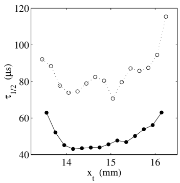
Figure 12: Half-time $\tau_{\scriptscriptstyle{1/2}}$ of the homodyne correlation function vs. position in the gap for a well-focussed collection optics $d_{FL}=0$ ($\circ$) and for a defocussed case $d_{FL}\simeq 200~{}\mu$m ($\bullet$). For each data point, the correlation function was accumulated over 1 min. The shear rate was set to $\dot{\gamma}=10$ s^-1.

4.4.2 Experimental features of heterodyne DLS under shear

In order to extract the Doppler shift $\mathbf{q}\cdot\mathbf{v}$ from the experimental heterodyne correlation function, we interpolate the experimental curves as shown in Fig. 9. A series of cancellation times $\tau_{k}$ is extracted from the interpolation. The $\tau_{k}$’s are marked by $\times$ symbols in Fig. 9. Since $C(\tau)\propto F(\tau)\,\cos(\mathbf{q}\cdot\mathbf{v}\tau)$, one expects $\tau_{k}=(k\pi+\frac{\pi}{2})(\mathbf{q}\cdot\mathbf{v})^{-1}$ provided $F(\tau)$ does not vanish. It is then straightforward to estimate the scalar product $\mathbf{q}\!\cdot\!\mathbf{v}$ from a linear fit of $\tau_{k}$ vs. $k$.

To obtain velocity profiles, one has to move the scattering volume across the gap of the Couette cell. This is done by moving the rheometer in the $x$ direction with the help of the mechanical table (cf. Fig. 4). The Doppler period $T=(\mathbf{q}\!\cdot\!\mathbf{v})^{-1}$ is plotted for different positions $x_{t}$ of the table and for different imposed shear rates in Fig. 13(a). To estimate the velocity corresponding to a given Doppler period, one has to know precisely the scattering vector $\mathbf{q}$. As explained in Sec. 4.2 refraction leads to important optical corrections. Indeed the real scattering angle $\theta$ differs from the imposed angle $\theta_{i}$ since $\theta\approx f_{\theta}\theta_{i}$, where $f_{\theta}\approx 0.79$. Such a correction allows us to convert the measured period $T$ into a velocity $v$ as shown in Fig. 13(b). Indeed, assuming that $\mathbf{v}=v\,\mathbf{e}_{y}$, i.e. that the flow is purely orthoradial in the $(x,y)$ plane, $\mathbf{q}\!\cdot\!\mathbf{v}=qv\cos(\theta/2)=2\pi n\sin\theta\,v/\lambda$.

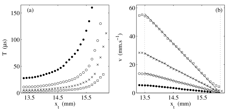
Figure 13: Calibration of the velocity measurements using a Newtonian suspension of latex spheres in a water-glycerol mixture submitted to different shear rates $\dot{\gamma}=2$ s${}^{-1}~{}(\bullet)$, 5 s${}^{-1}~{}(\circ)$, 10 s${}^{-1}~{}(\times)$, and 20 s${}^{-1}~{}(\Box)$. (a) Raw estimates of the period $T$ of the oscillations in the heterodyne correlation function as a function of the position of the mechanical table $x_{t}$. The origin of $x_{t}$ is arbitrary and is defined when the actuators are first initialized. (b) Velocity estimates using the procedure described in Sec. 4.4.2. Each data set is fitted by a straight line, which yields an estimate for the position of the fixed outer wall: $x_{f}=16.15\pm 0.02$ mm (dotted line). The dotted line at $x_{m}=13.49$ mm shows the estimated position of the moving inner wall. The solid lines are the linear velocity profiles $v=(R_{\scriptscriptstyle 1}\dot{\gamma}/F_{\dot{\gamma}})\,(x_{f}-x_{t})/(x_{f}-x_{m})$ with $\dot{\gamma}=2$, 5, 10, and 20 s^-1.

Linear fits of the measured velocity profiles allow us to estimate the position of the fixed outer wall $x_{f}=16.15$ mm with a precision of about $20~{}\mu$m. The velocity $v_{\scriptscriptstyle 0}$ of the rotor is given by the rheometer: for a given angular velocity $\Omega$ of the rotor, the shear rate $\dot{\gamma}$ indicated by the rheometer, $\dot{\gamma}=F_{\dot{\gamma}}\Omega$ where $F_{\dot{\gamma}}=(R_{\scriptscriptstyle 1}^{2}+R_{\scriptscriptstyle 2}^{2})/(R_{\scriptscriptstyle 2}^{2}-R_{\scriptscriptstyle 1}^{2})$ with $R_{\scriptscriptstyle 1}$ and $R_{\scriptscriptstyle 2}$ denoting the radii of the rotor and the stator of the Couette cell. $F_{\dot{\gamma}}$ is a conversion factor inherent to the rheometer that account for the Couette geometry. The velocity of the mobile inner wall is thus given by: $v_{\scriptscriptstyle 0}=R_{\scriptscriptstyle 1}\Omega=R_{\scriptscriptstyle 1}\dot{\gamma}/F_{\dot{\gamma}}$. This permits the determination of the position of the moving inner wall $x_{m}=13.49$ mm (left dashed line in Fig. 13(b)). Such a determination leads to an effective gap width $e^{\prime}=x_{f}-x_{m}\approx 2.65$ mm, which differs from the real gap $e=3$ mm. Actually as shown in Sec. 4.2, the actual displacement of the scattering volume inside the cell $\delta x^{\prime}$ is related to the displacement of the mechanical table $\delta x$, by the following relation: $\delta x^{\prime}=f_{x}\delta x$, where $f_{x}\approx 1.13$ is deduced from the Snell-Descartes law for refraction. Such a conversion factor is in excellent agreement with the previous result since $e/e^{\prime}\approx 1.13$. Let us notice that for all the imposed shear rates, we were able to measure velocities for a few points that are outside the gap at $x_{t}<x_{m}$ (see Fig. 13(b)). This is due to the finite extent of the scattering volume: even for $x_{t}<x_{m}$, some small intensity may be detected that is scattered from the intersection of the scattering volume and the gap.

In the velocity profiles displayed in Fig. 14, the two optical conversion factors $f_{\theta}$ and $f_{x}$ have been taken into account and $x$ denotes the real position inside the gap. In all cases, the uncertainty of the experimental measurements is of the order of the marker size. Note that the effect of non-homogeneous shear rate due to the curved geometry of the Couette cell is negligible for such a Newtonian fluid and does not influence the calibration.

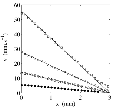
Figure 14: Velocity profiles in a sheared Newtonian suspension for $\dot{\gamma}=2$ s${}^{-1}~{}(\bullet)$, 5 s${}^{-1}~{}(\circ)$, 10 s${}^{-1}~{}(\times)$, and 20 s${}^{-1}~{}(\Box)$. The abscissa $x$ denotes the real position within the cell gap. The origin of $x$ is taken at the inner wall. The solid lines are the linear velocity profiles $v=R_{\scriptscriptstyle 1}\dot{\gamma}(1-x/e)/F_{\dot{\gamma}}$ with $\dot{\gamma}=2$, 5, 10, and 20 s^-1. The conversion factors $f_{\theta}=0.79$ and $f_{x}=1.13$ are used to account for refraction effects

4.4.3 Spatial resolution

One of the most relevant features of a technique measuring velocity profiles is its spatial resolution. As previously outlined, a good resolution would be around $100~{}\mu$m. In our case, spatial resolution is limited by the size of the scattering volume $\mathcal{V}$. Indeed, velocity measurements using heterodyne DLS are averaged over $\mathcal{V}$. The typical dimensions of $\mathcal{V}$ in air are $a\approx 20~{}\mu$m and $c^{\prime}\approx 40~{}\mu$m measured in Sec. 4.3.2. Since scattering occurs at an angle $\theta$ and since the Couette cell acts as a lens, the relevant size is $c\approx f_{x}c^{\prime}/\sin(f_{\theta}\theta_{i})$, which leads to a typical size $c\approx 100~{}\mu$m. However, the spatial resolution of our setup strongly depends on the scattering angle. The latest measurements performed in our group on banded flows in micellar solution at a larger angle ($\theta_{i}\approx 50^{\circ}$) reveal that our setup can resolve a discontinuity of the shear rate with an accuracy of about $50~{}\mu$m Molino:02 .

4.4.4 Temporal resolution

As recalled in the Introduction, some complex fluids display non-stationnary flows Bandyopadhyay:01 ; Salmon:02 . Therefore it is interesting to perform time-resolved measurements of the local velocity. To obtain the Doppler frequency with a high temporal resolution one may use a spectrum analyzer rather than a correlator. Such a technique allows up to a thousand measurements per second. For instance, this has been implemented long ago by Gollub et al. to measure the temporal evolution of the local velocity in Newtonian fluids at the onset of the Taylor-Couette instability Gollub:75 . However the use of a correlator yields more information than a spectrum analyzer. In homodyne mode qualitative information on the local shear rate can be obtained, as discussed in Secs. 3 and 4.4.1. Moreover, the use of a correlator once the shear flow has been stopped can give important information on the coupling between the structural dynamics of a material and an applied shear Viasnoff:02 .

The temporal resolution of our setup strongly depends on the power of the laser beam and on the quantity of light scattered by the sample. Actually these two features control $N(t)$, the number of photons detected by the photomultiplier tube per second. To estimate the temporal resolution of our setup, we measured the homodyne and heterodyne correlation functions for various accumulation times $t_{a}$ at a given $N(t)$. Then we computed the corresponding half-times of the homodyne correlation functions and the Doppler periods in the heterodyne mode. Figure 15 displays such measurements obtained on a latex suspension in the middle of the gap for $\dot{\gamma}=10$ s^-1 and with $N(t)\approx 10^{4}$ events per second in homodyne mode. The error bars represent the standard deviations of different measurements obtained at a given accumulation time $t_{a}$. It clearly appears that good statistical estimates of $\tau_{\scriptscriptstyle{1/2}}$ and $T=(\mathbf{q}\!\cdot\!\mathbf{v})^{-1}$ are obtained after an accumulation time of the order of $5$ seconds. Actually in better experimental conditions, for instance when $N(t)\approx 3.10^{4}$, the accumulation time required to define those characteristic times decreases to $1$ second. Therefore our setup is well suited to follow dynamics like those observed in Refs. Bandyopadhyay:01 ; Salmon:02 that involve time scales in the range 1–$10^{3}$ s.

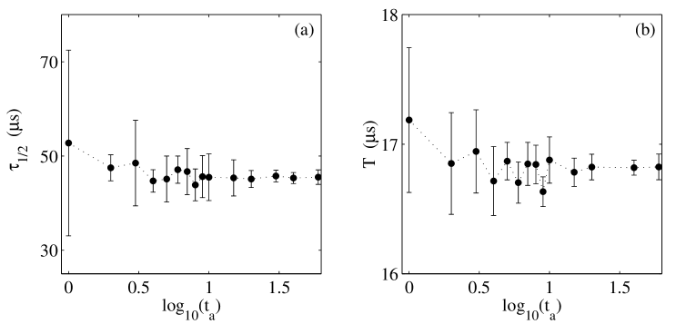
Figure 15: Statistical convergence of the estimates of the characteristic times. (a) Half-time $\tau_{1/2}$ of the homodyne correlation function vs. accumulation time $t_{a}$. (b) Period $T$ of the oscillations in the heterodyne correlation function vs. accumulation time $t_{a}$. Each data point represents the average over the the characteristic times estimated from five consecutive correlation functions accumulated over $t_{a}$. The error bars account for the standard deviation of those five measurements. The shear rate was set to $\dot{\gamma}=10$ s^-1.

5 Discussion and conclusion

In this article, we presented an experimental setup based on the use of single mode fibers that allows one to measure velocity profiles in Couette flows. We have shown that measurements of the local shear rate using homodyne DLS are difficult to implement in the Couette geometry. By measuring directly the shape of the scattering volume, we were able to compare experimental and theoretical homodyne correlation functions, and show that the decorrelation times $\tau_{\scriptscriptstyle{1/2}}$ are linked to the size of the scattering volume $c$ and to the local shear rate $\dot{\gamma}$ according to $\tau_{\scriptscriptstyle{1/2}}\propto 1/(c\dot{\gamma})$ as expected from theory.

Heterodyne detection yields the Doppler shift $\mathbf{q}\cdot\mathbf{v}$ associated to the average velocity in the scattering volume. Provided refraction effects are taken into account and a careful calibration is performed, our setup gives access to velocity profiles in Couette flows of complex fluids down to a spatial resolution of 50 $\mu$m. As far as temporal resolution is concerned, the major limitation is the time required to move the rheometer along the direction of shear. In the best experimental conditions and with about $30$ points in the gap of the Couette cell, we managed to measure velocity profiles in about one minute. Thus, our setup cannot resolve flow dynamics over the whole gap on time scales shorter than one minute. Other non intrusive techniques like ultrasonic speckle correlation recently developed in our group may allow us to measure up to $10^{2}$ velocity profiles per second and may yield rich information on faster dynamics.

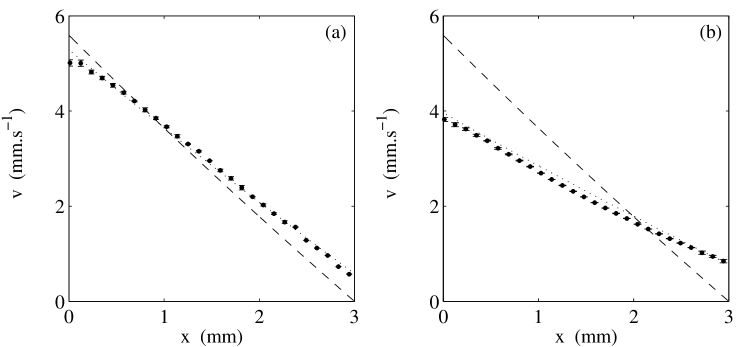
Figure 16: Velocity profiles for $\dot{\gamma}=2$ s^-1 in two different emulsions. (a) Dilute emulsion $\phi=20~{}\%$. (b) Concentrated emulsion $\phi=75~{}\%$. The dashed lines represent the velocity profiles expected for a Newtonian fluid. The dotted lines correspond to a Newtonian fluid when wall slip has been taken into account

In order to show its relevance in the field of complex fluid flows, the DLS technique described in this paper was applied to sheared emulsions. Figure 16 shows the velocity profiles measured in two different oil-in-water emulsions at the same shear rate. The Couette cell is that used throughout this study ($e=3$ mm and $R_{\scriptscriptstyle 1}=22$ mm). Both emulsions are composed of silicone oil droplets (diameter $\approx 2~{}\mu$m) in a water–glycerol mixture with 1 % TTAB surfactant. Figure 16(a) corresponds to a dilute emulsion of volume fraction $\phi=20~{}\%$ whereas Fig. 16(b) was obtained with a concentrated system of volume fraction $\phi=75~{}\%$. For $\dot{\gamma}=2$ s^-1, rheological data recorded by the rheometer show that the global stresses imposed on the samples are $\sigma=0.07$ Pa and $\sigma=290$ Pa respectively. The optical index $n$ of the aqueous phase is matched to that of the silicone oil to avoid multiple scattering. Moreover, $n=1.40$ as in the latex suspension used for the calibration, so that the values of $f_{x}$ and $f_{\theta}$ discussed in Sec. 4.2 and 4.4.2 remain valid in the case of those emulsions. In both cases, slippage clearly shows on the velocity profiles when compared to that of a Newtonian fluid. Wall slip is much larger for the concentrated system. Moreover, the velocity profile is almost perfectly linear in the dilute emulsion (see fig. 16(a)) whereas a small but systematic curvature can be noticed in the concentrated emulsion (see fig. 16(b)). This curvature is the signature of the non-Newtonian behavior of the 75 % emulsion. The complete analysis of the slip velocities and of the bulk flow behavior inferred from such local measurements will be discussed at length in a related publication Salmon:02_3 .

Finally, the main innovation of the present work is to provide both local velocity measurements and global rheological data simultaneously. DLS coupled to standard rheology opens the door to local rheology. Indeed, when the flow is stationnary, the local stress in a Couette cell is inversely proportional to the square of the position in the gap. On the other hand, the local shear rate may be accessed by differentiating the velocity profiles. Thus, we could determine the relationship between the local shear rate and the local stress and define a local flow behaviour. The comparison between such a local rheology and the global flow curve obtained with a standard rheometer should lead to essential knowledge that may prove crucial to understand complex fluid flows Fisher:01 ; Salmon:02_3 ; Molino:02 ; Coussot:02 .

- (1) M. E. Cates and M. R. Evans, editors. Soft and Fragile Matter: Non Equilibrium Dynamics Metastability and Flow. Institute of Physics Publishing (Bristol), 2000.
- (2) R. G. Larson. The structure and rheology of complex fluids. Oxford University Press, 1999.
- (3) P. Sollich, F. Lequeux, P. Hébraud, and M. E. Cates. Rheology of soft glassy materials. Phys. Rev. Lett., 78:2020, 1997.
- (4) V. Viasnoff and F. Lequeux. Rejuvenation and overaging in a colloidal glass under shear. Phys. Rev. Lett., 89:065701, 2002.
- (5) A. Spenley, M. E. Cates, and T. C. B. McLeish. Nonlinear rheology of wormlike micelles. Phys. Rev. Lett., 71:939, 1993.
- (6) J.-F Berret, G. Porte, and J.-P. Decruppe. Inhomogeneous shear flows of wormlike micelles: A master dynamic phase diagram. Phys. Rev. E, 55:1668, 1997.
- (7) D. Roux, F. Nallet, and O. Diat. Rheology of lyotropic lamellar phases. Europhys. Lett., 24:53, 1993.
- (8) M. M. Britton and P. T. Callaghan. Two-phase shear band structures at uniform stress. Phys. Rev. Lett., 78:4930, 1997.
- (9) E. Fischer and P. T. Callaghan. Shear banding and the isotropic-to-nematic transition in wormlike micelles. Phys. Rev. E, 64:011501, 2001.
- (10) A.-S. Wunenburger, A. Colin, J. Leng, A. Arnéodo, and D. Roux. Oscillating viscosity in a lyotropic lamellar phase under shear flow. Phys. Rev. Lett., 86:1374, 2001.
- (11) R. Bandyopadhyay and A. K. Sood. Chaotic dynamics in shear-thickening surfactant solutions. Europhys. Lett., 56:447–453, 2001.
- (12) J.-B. Salmon, A. Colin, and D. Roux. Dynamical behavior of a complex fluid near an out-of-equilibrium transition: Approaching simple rheological chaos. Phys. Rev. E, 66:031505, 2002.
- (13) M. E. Cates, D. A. Head, and A. Ajdari. Rheological chaos in a scalar shear-thickening model. Phys. Rev. E, 66:025202, 2002.
- (14) S. J. Muller, R. G. Larson, and E. S. G. Shaqfeh. A purely elastic transition in taylor-couette flow. Rheol. Acta, 28:499, 1989.
- (15) A. Groisman and V. Steinberg. Elastic turbulence in a polymer solution flow. Nature, 405:53, 2000.
- (16) H. A. Barnes. A review of the slip (wall depletion) of polymer solutions, emulsions and particle suspensions in viscometers: its cause, character, and cure. J. Non-Newtonian Fluid Mech., 56:221, 1995.
- (17) S. Sanyal, D. Yavich, and L. G. Leal. Dynamics of entangled polymeric fluids in two-roll mill studied via dynamic light scattering and two-color flow birefringence. i. steady flow. E-print cond-mat/0006275, 2000.
- (18) S. E. Welch, M. R. Stetzer, G. Hu, E. B. Sirota, and S. H. J. Idziak. Intermembrane spacing and velocity profiling of a lamellar lyotropic complex fluid under flow using x-ray diffraction. Phys. Rev. E, 65:061511, 2002.
- (19) G. Debrégeas H. Tabuteau and J.-M di Meglio. Deformation and flow of a two-dimensional foam under continuous shear. Phys. Rev. Lett., 87:178305, 2001.
- (20) J.-B. Salmon, L. Bécu, S. Manneville, and A. Colin. Towards local rheology of emulsions under couette flow using dynamic light scattering. Submitted to Eur. Phys. J. E, 2002.
- (21) B. J. Berne and R. Pecora. Dynamic light scattering. Wiley, New York, 1995.
- (22) F. Nallet, D. Roux, and J. Prost. Dynamic light scattering study of dilute lamellar phases. Phys. Rev. Lett., 62:276, 1988.
- (23) J. J. Wang, D. Yavich, and L. G. Leal. Time-resolved velocity gradients and optical anisotropy in linear flow by photon correlation spectroscopy. Phys. Fluids, 6:3519, 1994.
- (24) B. J. Ackerson and N. A. Clark. Dynamic light scattering at low rates of shear. J. Physique, 42:929, 1981.
- (25) J. P. Gollub and M. H. Freilich. Optical heterodyne study of the taylor instability in a rotating fluid. Phys. Rev. Lett., 33:1465–1468, 1974.
- (26) J. P. Gollub and H. L. Swinney. Onset of turbulence in a rotating fluid. Phys. Rev. Lett., 35:927, 1975.
- (27) G. G. Fuller, J. M. Rallison, R. L. Schmidt, and L. G. Leal. The measurements of velocity gradients in laminar flows by homodyne light-scattering spectroscopy. J. Fluid Mech., 100:555, 1980.
- (28) K. J. Måløy, W. Goldburg, and H. K. Pak. Spatial coherence of homodyne light scattering from particles in a convective velocity field. Phys. Rev. A, 46:3288, 1992.
- (29) F. Molino, J.-B. Salmon, S. Manneville, and A. Colin. Evidence for shear-banding in wormlike micelles with dynamic light scattering. To be published.
- (30) P. Coussot, J. S. Raynaud, F. Bertrand, P. Moucheront, J. P. Guilbaud, H. T. Huynh, S. Jarny, and D. Lesueur. Coexistence of liquid and solid phases in flowing soft-glassy materials. Phys. Rev. Lett., 88:218301, 2002.