Molecular dynamics simulations of crystallization of hard spheres

Abstract

We have carried out molecular dynamics simulations of the crystallization of hard spheres modelling colloidal systems that are studied in conventional and space-based experiments. We use microscopic probes to investigate the effects of gravitational forces, polydispersity and of bounding walls on the phase structure. The simulations employed an extensive exclusive particle grid method and the type and degree of crystalline order was studied in two independent ways: by the structure factor, as in experiments, and through local rotational invariants. We present quantitative comparisons of the nucleation rates of monodisperse and polydisperse hard sphere systems and benchmark them against experimental results. We show how the presence of bounding walls leads to wall-induced nucleation and rapid crystallization and discuss the role of gravity on the dynamics of crystallization.

I Introduction

Hard sphere systems are idealized approximations to a large number of physical systems, such as simple liquids Hansen and McDonald (1986), glasses Zallen (1983), colloidal dispersions Torquato and Lado (1986) and particulate composites Bernal (1959) and are now being studied extensively in a microgravity environment Zhu et al. (1997); Cheng et al. (2002); Sankaran et al. (2001) which allows for a creation of new technological materials, such as photonic crystals Rudhardt et al. (2000). The use of colloidal particles for engineering new materials is a relatively unexplored field which promises to revolutionize materials synthesis. Colloidal suspensions are also interesting from a fundamental scientific point of view since they self-assemble into a wide range of structures. Thus, they may be thought of as models of atomistic condensed matter systems with the distinct advantage of relevant length and time scales being more readily accessible to experiments.

On Earth, the effects of sedimentation and gravity-induced convection can cloud, modify, or sometimes even radically alter, the intrinsic behavior of certain classes of colloidal systems. Because the binding energies of the crystalline phases are low and comparable to each other, gravity can greatly influence the kinetics of formation and, indeed, the very nature of the observed crystal structure. Colloidal suspensions of hard spheres are model systems for studying the statistical mechanics of structural phase transitions. Such suspensions undergo an entropy-driven phase transition from fluid to crystal as a function of increasing volume fraction. Unlike comparable phase transitions in conventional systems of condensed matter, the dynamics of such structural phase transitions can be monitored with “atomic” precision using conventional light microscopy. In hard sphere systems, at high volume fractions, glass formation competes with the nucleation and growth of the crystalline phase. The Chaikin-Russel experiments on the Space Shuttle Zhu et al. (1997); Cheng et al. (2002) have led to the striking result that samples of hard sphere colloids that remain glassy on the Earth for more than a year crystallize within a few weeks in a microgravity environment.

In this paper, we present results of molecular dynamics (MD) simulations of the crystallization of hard spheres. These simulations allow for microscopic probes of the physics involved in both conventional and space-based measurements of nucleation and crystal growth in colloidal systems. We focus on the effects of weak gravitational forces, polydispersity and on the effects of bounding walls on phase structure. We present quantitative comparisons of the nucleation rates of monodisperse and polydisperse hard sphere systems and benchmark them against experimental results. We demonstrate that the presence of gravity can delay crystallization. Furthermore, we show how the presence of the bounding walls leads to wall-induced nucleation and rapid crystallization.

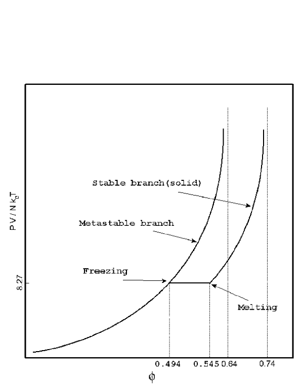
Figure 1: Schematic representation of the phase diagram of a system of hard spheres.

Numerical studies of the hard sphere system started with the pioneering work of Alder and Wainwright Adler and Wainwright (1957). Since then, there have been many studies that elucidated the nature of the phase diagram. In particular, computer simulations(see Rintoul and Torquato (1996); Wood and Jacobson (1957); Hoover and Ree (1968); Speedy (1994) for a few examples) have provided evidence for the existence of a first order fluid-to-solid transition in the hard sphere system. With an increase of the packing fraction, $\phi$, (defined as the ratio of the volume occupied by the spheres to the total volume) the system in the liquid state reaches the freezing point at $\phi=49.4\%$ (see Fig. 1 for a sketch). The phase diagram splits into metastable and stable branches at this point. The metastable branch is a continuation of the liquid branch and it exists in the region between the freezing point and $\phi\approx 64\%$ which corresponds to the random close packing (rcp) state. The rcp provides the maximum $\phi$ that can be achieved in the disordered system. The stable branch consists of a coexistence region of liquid and crystal which ends at $\phi$ of $54.5\%$ corresponding to the melting point. Above the melting point, the stable branch represents the crystal state and that is present up to $\phi\approx 74\%$ which corresponds either to the close packed face-centered cubic (fcc) or to the hexagonal closed packed (hcp) configurations.

The metastable branch, especially its part above the melting point, has received a lot of attention in the last several years. One of the debated issues here is the existence of the glassy state in the metastable system when $\phi>58\%$, i.e. in the vicinity of the rcp value. A number of papers report no sign of crystallization Speedy (1994); Yeo (1995); van Blaaderen and Wiltzius (1995) and thus confirm the presence of the glassy state. On the other hand, Rintoul and Torquato Rintoul and Torquato (1996) have argued that if computer simulations were to run for a sufficiently long time, then crystallization would eventually set in. A striking experimental evidence for this scenario has been provided by a recent microgravity experiment on the Space Shuttle Zhu et al. (1997). It demonstrated crystallization in a hard sphere colloidal dispersion at $\phi=61.9\%$ occurring on the time scale of several days whereas the same system stayed amorphous for more than a year when studied on Earth.

The formation of the crystals in the supersaturated hard-sphere system is commonly described by the classical nucleation theory (see Anderson and Lekkerkerker (2002) and references therein). According to this theory, a crystallite forms in the system due to thermal fluctuations and then its total free energy consists of two terms: a negative bulk term, which is proportional to the volume of the crystallite, and a positive surface term which is proportional to its surface area. This leads to the prediction that the crystallite will continue to grow only when its size is bigger than a certain critical value and it will shrink otherwise. There are a number of experimental results that support the classical nucleation theory Anderson and Lekkerkerker (2002); Harland and van Megen (1997).

The MD simulations of the hard spheres systems that we report on in this paper are focused on the dynamics of crystallization above the melting concentration and are complementary to the earth-based studies of Gasser et al. Gasser et al. (2001). The crystallization process is monitored by means of local order parameters as well as through the static structure factor. The former method is currently widely used to analyze the results of computer simulations whereas the structure factor is measured experimentally. We investigate the influence of bounding walls, polydispersity and of gravitational field on the dynamics of crystallization and show that the nucleation rates for crystallization are comparable to the values obtained experimentally.

We show that the system with periodic boundary conditions crystallizes in a somewhat complex manner with an interconnected phase of growing crystal nuclei. In contrast, a system with planar walls exhibits layering and leads to a heterogeneous wall nucleation mechanism characterized by more rapid crystallization. For volume fraction around $56\%$, gravity leads to a concentration gradient accompanied by the formation of very well-defined layers with excellent planar ordering. However, at larger volume fractions, gravity causes the crystallization process to slow down relative to the planar wall case without any imposed gravitational field. Polydispersity in the size distribution of the hard spheres leads to slower crystallization and in the absence of gravity, we found an increase with time of the relative fraction of hard spheres with fcc order compared to hcp suggesting that the former crystal structure is preferred to the latter.

The outline of the paper is as follows. In Section II, we describe the algorithms used in the simulations. In Section III, we present the methods of the analysis of the local structure and of the thermodynamical properties of the system. Section IV presents the results of our simulations for both monodisperse and polydisperse systems with periodic boundary conditions. Section V considers the effects arising due to rigid flat walls that restrict motion in one direction and discusses the role of a uniform gravitational field along this direction. Finally, in Section VI, we discuss the nature of the crystalline phase.

II The MD simulation

There are many possible algorithms that can be used in the MD simulations of hard sphere systems Allen and Tildesley (1987). Owing to the simplicity of the potential, the only events that need to be calculated are the consecutive collisions between the particles. In this respect, the MD algorithms for the hard sphere systems are quite distinct from the algorithms for the soft types of potentials where the evolution between the collisions also matters. Thus the evolution should not be considered in equal time steps but instead it ought to be studied through an event driven algorithm. The most challenging part of such an algorithm, in terms of its computational performance, is the proper scheduling of the future collisions and the organization of the data structure.

Our MD simulations were performed by implementing the algorithms proposed by Isobe Isobe (1999) who introduced the concept of an extended exclusive particle grid method to the studies of hard sphere and hard disk systems. In this method, the volume $V$ containing the particles is divided into small cells, so that each cell contains no more than one particle. Thus, the continuous coordinates of the particles are “mapped” onto a lattice which allows for an easy specification of neighboring particles. Candidates for the next particle-pair collision are found just by searching the neighboring cells. Once this is accomplished, the next collision event for the system can be found by creating a complete binary tree Marin et al. (1993). The positions of all the particles do not need to be updated after each collision, since in a sufficiently dense system the neighborhood of a particle remains the same for a long time.

The initial packing of the system of $N$ hard spheres was generated from a random set of points within a box by using an iterative algorithm proposed by Jullien et al. Jullien et al. (1996). At each stage of this algorithm one identifies the pair of particles with the smallest mutual distance $d_{m}^{i}$ (the superscript $i$ refers to the $i$th stage of the iterative procedure) and moves them apart symmetrically by a distance $d_{M}^{i}$ which decreases with each iterative step according to the following formula:

$$d_{M}^{i+1}=d_{M}^{i}-{\hat{R}\over N}\left(\phi_{M}^{i}-\phi_{m}^{i}\right)^{1/3}\;\;.$$ (1)

Here $\phi_{M,m}^{i}=\pi d_{M,m}^{3}N/(6V)$, $\phi_{M}^{0}=1$, and $\hat{R}$ is a parameter of the algorithm. The process continues until $d_{M}<d_{m}$ and the final value of $d_{m}$ is chosen to be the particle diameter. Different values of $\hat{R}$ lead to different packing fractions and generally, the smaller the $\hat{R}$, the larger the packing fraction. In the limit of $\hat{R}\rightarrow 0$, one reaches a packing fraction corresponding to the random close packed value. In order to obtain a polydisperse distribution of the radii we modified this algorithm so that at each iteration step we move apart two particles that overlap the most and their new mutual distance is set equal to the sum of the predefined particles’ radii.

Our MD simulations were performed with at least $10976$ hard spheres (both in the mono- and polydisperse cases). The particles were placed in a cubic box. In the absence of any walls, periodic boundary conditions were imposed. When studying the effects of the walls, two flat walls were introduced at $z=0$ and $z=L$ while maintaining the periodic boundary conditions in the other two directions. This was accomplished by changing the standard algorithm Jullien et al. (1996) so that the walls are represented by two new “particles” which do not move. The initial particle velocities were chosen to be random with a Gaussian distribution and zero total momentum.

The results were averaged over six simulations for each set of control parameters. We have focused on the concentration range from $\phi=54\%$ to $\phi=58\%$ for systems without the bounding walls and gravity and from $\phi=54\%$ to $\phi=63\%$ in the other cases. This procedure was motivated by the fact that for lower and higher concentrations the crystallization times increase substantially and so does the computational time.

In our simulations we define the hard sphere diameter to be $1$ unit and the timescale is defined by choosing the the mean absolute velocity of the hard spheres to be $1$. Following the approach of Harland and van Megen Harland and van Megen (1997), in order to make contact with experiment, we show the results of our simulations by expressing times and lengths in units of the diffusional characteristic time $\tau_{b}=R^{2}/D_{0}$ and hard sphere diameter $2R$, respectively. Here, $\displaystyle{D_{0}={3\pi\over 16\sqrt{2}}\bar{v}l_{mfp}}$, where $\bar{v}$ is the mean absolute velocity of the hard spheres and the mean free path $\displaystyle{l_{mfp}={V\over N4\pi R^{2}}}$. The acceleration due to the gravity was chosen to be approximately $4.7$ (see caption in Figure 12 for precise values) in units in which the hard sphere diameter is $1$ and the mean absolute velocity is $1$.

III Characterization of the hard sphere systems

III.1 The equation of state

The relevant parameter that describes the thermodynamic properties of the hard sphere system is the pressure, $P$, since the internal energy of such a system is that of an ideal gas. Changing the temperature, $T$, is simply equivalent to rescaling the time scale. The pressure can be calculated by using the radial distribution function or through the collision rate in the system. The latter method is more reliable because of the difficulties with a precise determination of the radial distribution function.

The equation of state in terms of the collision rate $\Gamma$ is given by Hoover and Alder (1967)

$${PV\over Nk_{B}T}=1+{\Gamma\over\Gamma_{0}}{B_{2}\over V}\;\;,$$ (2)

where $V$ is the total volume, $N$ the number of particles, $k_{B}$ the Boltzmann’s constant, $B_{2}$ the second virial coefficient. $\Gamma_{0}$ is the low-density collision rate which is given by Alder and Wainwright (1960)

$$\Gamma_{0}=8{N(N-1)\over V}R^{2}\sqrt{\pi<v^{2}>\over 3}\;\;,$$ (3)

where $<v^{2}>$ is the mean square velocity and $R$ the radius of the sphere.

The pressure was monitored throughout the simulation and was used as a quantitative parameter which allowed us to check on the progress of the crystallization.

III.2 The local structure

A number of methods has been used in the literature to characterize the local structure and a degree to which it is crystalline. A widely used technique to distinguish between crystalline and amorphous structures is through the Voronoi analysis of the topology of the neighborhood of a given particle. The Voronoi polyhedron is defined Zallen (1983) as the set of all points that are closer to a given particle than to any other. Partitioning of space into the Voronoi polyhedra allows one to make a natural identification of the neighbors. Determination of the numbers of walls in the Voronoi polyhedra leads to an unambiguous selection of the particles in the solid-like regions. However, such an analysis lacks precision when applied to thermally distorted crystals and is not too effective in distinguishing between various types of crystalline order. The same difficulties arise when the structure, crystalline or not, is analyzed through the particle distribution function.

III.2.1 The local invariants

In order to determine the kind of the local order around a particle and to distinguish between the fcc, hcp, bcc and liquid-like configurations we make use of the local order parameter method Steinhardt et al. (1983); Mitus et al. (1995), which gives reliable results even in the case of crystalline structures which are highly perturbed. The first step here is to construct the normalized order parameter $\hat{q}_{lm}$ for a particle $i$ through

$$\hat{q}_{lm}(i)={1\over N_{b}(i)}\sum_{j=1}^{N_{b}(i)}Y_{lm}(\vec{r}_{ij})\;\;,$$ (4)

where $N_{b}(i)$ is the number of neighbors of the particle, $Y_{lm}$ is a spherical harmonic and $\vec{r}_{ij}=\vec{r}_{j}-\vec{r}_{i}$ with $\vec{r}_{i}$ being the coordinates of the center of particle $i$. The neighbors are defined to be those particles which have a mutual distance less than a certain cutoff value. It is physically appealing to choose the cutoff as corresponding to the position of the first minimum in the radial distribution function. $Y_{lm}$ is the spherical harmonic function which means that $\hat{q}_{lm}(i)$ has $2l+1$ complex components. $\hat{q}_{lm}(i)$ can be normalized by multiplication of a suitable constant to yield $\bar{q}_{lm}(i)$, such that

$$\sum_{m=-l}^{m=l}\bar{q}_{lm}(i)\bar{q}_{lm}^{*}(i)=1\;\;.$$ (5)

If

$$\left|\sum_{m=-l}^{m=l}\bar{q}_{lm}(i)\bar{q}_{lm}^{*}(j)\right|>0.5$$ (6)

then the bond between particles $i$ and $j$ is considered to be crystal-like. Furthermore, if a particle has seven or more crystal-like bonds, then it is counted as belonging to a crystalline region. Note, that $\bar{q}_{lm}(i)$ is not rotationally invariant and hence the quantity on the left hand side of Eq. (6) depends on the choice of the coordinate axes. Indeed, for a given bond, there can be ambiguity about whether the quantity in Eq. (6) is greater than the threshold value of $0.5$ or not. However, when summing over all the bonds connected to a given hard sphere, the criterion for crystallinity is substantially independent of the choice of the coordinate axes.

In order to distinguish between different crystal structures we construct the second-order rotational invariants $q_{4}(i)$, $q_{6}(i)$, and $\hat{w}_{6}(i)$ ten Wolde et al. (1996), where

$$q_{l}(i)=\left[{4\pi\over 2l+1}\sum_{m=-l}^{m=l}|\hat{q}_{lm}(i)|^{2}\right]^{1\over 2}\;\;$$ (7)

and

$$\hat{w}_{l}(i)=\mathop{\sum_{m_{1},m_{2},m_{3}}}_{m_{1}+m_{2}+m_{3}=0}\left(\begin{array}[]{ccc}l&l&l\\ m_{1}&m_{2}&m_{3}\\ \end{array}\right)\hat{q}_{lm_{1}}(i)\hat{q}_{lm_{2}}(i)\hat{q}_{lm_{3}}(i),$$ (8)

where $\left(\begin{array}[]{ccc}l&l&l\\ m_{1}&m_{2}&m_{3}\\ \end{array}\right)$ is a Wigner $3j$ symbol Edmonds (1974). After calculating $q_{4}(i)$, $q_{6}(i)$, $\hat{w}_{6}(i)$ one can decompose a vector $\vec{s}$ consisting of these three components into the five characteristic vectors $\vec{s}_{fcc}$, $\vec{s}_{hcp}$, $\vec{s}_{bcc}$, $\vec{s}_{sc}$ and $\vec{s}_{ico}$ corresponding to perfect fcc, hcp, bcc, sc, and icosahedral structures. The values for the perfect crystals are given in Table 1. Such a decomposition can be carried out by minimizing the following expression ten Wolde et al. (1995):

$$\Delta^{2}=\left[\vec{s}-(f_{fcc}\vec{s}_{fcc}+f_{hcp}\vec{s}_{hcp}+f_{bcc}\vec{s}_{bcc}+f_{sc}\vec{s}_{sc}+f_{ico}\vec{s}_{ico})\right]^{2}$$ (9)

with a constraint that all of the $f$ factors are positive and they add up to 1. As a result we get a set of five numbers $f$. Each $f$ represents the “importance” of the corresponding structure. For example, for each particle of the perfect fcc crystal we would get $f_{fcc}=1$ and all the others to be zero. For an imperfect crystal, we assign each particle to the structure corresponding to the biggest $f$. Note, that our method is slightly different from that used in Ref. ten Wolde et al. (1995) but in practice the two methods yield similar results. In Ref. ten Wolde et al. (1995), the clusters of particles were analyzed by comparing the distributions of the local order parameters for a given cluster and thermally equilibrated perfect crystals.

IV Dynamics of crystallization of mono- and polydisperse systems

We begin with an analysis of the crystallization process as monitored through the evolution of the Bragg peak in the static structure factor $S(q)$ Harland and van Megen (1997) where $q$ is the wave number. This method is widely used in analyzing data in the light scattering experiments.

After isolating the Bragg peak in the structure factor curve, we remove the liquid contribution by subtracting the Percus-Yevick result Ashcroft and Lekner (1966) multiplied by a constant which varies from $0$ (in the fully crystallized state) to 1 (in the liquid state) in order to ensure that $S(q)\rightarrow 0$ at small $q$. The crystal fraction, $X$, can be found by integrating the Bragg peak and choosing the upper limit of the integration at the minimum of $S(q)$ and by normalizing the result, so that $X=1$ in the fully crystallized state. The other parameters which can be determined in this approach are the average linear crystal size, $L=2K\pi/\Delta q$, where $K=1.155$ is the Scherrer constant for a crystal of a cubic shape James (1965), the number density of the crystals, $N_{c}=X/L^{3}$, and the nucleation density rate, $I=dN_{c}/dt$ Harland and van Megen (1997).

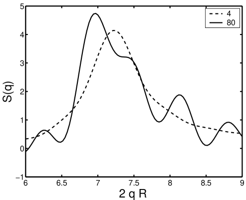
Figure 2: The dependence of the static structure factor on the wave number for $\phi=55\%$. The two curves shown correspond to the different stages of crystallization (after 4 and 80 steps where one step counts as 500 $\times N$ collisions, where $N$ is the number of particles). The dashed-line curve represents the Percus-Yevick solution (the liquid state, 4 steps) and the solid curve represents the fully crystallized system (80 steps).

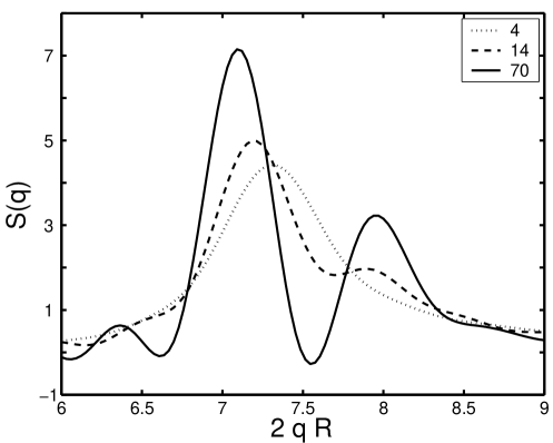
Figure 3: The dependence of the static structure factor on the wave number for $\phi=58\%$. The curves shown correspond to the three different stages of crystallization. The step numbers are indicated at the right hand corner.

An example of the time variation of the static structure factor for the monodisperse system (at $\phi=55\%$) is shown in Fig. 2. One observes that the structure factor exhibits the expected dynamics, namely, the Bragg peak at $2qR\approx 7$ corresponding to the $\{111\}$ direction becomes higher and higher and it shifts to lower wave numbers on crystallization. However, it is difficult to isolate the Bragg peak due to the emergence of other peaks, for instance, of the one corresponding to the fcc structure ($\{200\}$ peak). Note, that the shape of the structure factor on the left hand side of the Bragg peak remains substantially unchanged. Therefore, for the analysis of the structure, we used only the left half of the Bragg peak and then multiplied the results by a factor of two. For example, in Fig. 2, the lower integration limit was taken to be 6.5 and the upper one at the maximum of the Bragg peak. At higher packing fractions, we observed distinctive Bragg peaks at all stages of crystallization (Fig. 3).

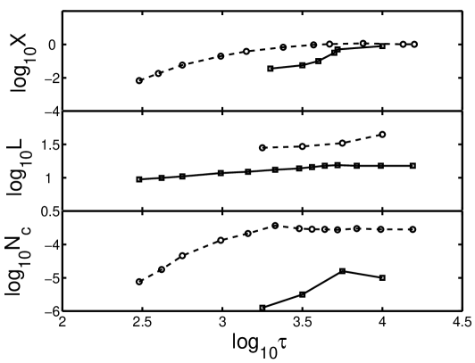
Figure 4: The time evolution of the crystal fraction $X$(top panel), the average linear crystal size $L$ (in particle diameters, middle panel), and the number density of the crystals $N_{c}$ (in units of $(2R)^{-3}$, bottom panel) for the monodisperse system at $\phi=55\%$. Our results are shown as solid lines and the experimental results Harland and van Megen (1997) as dashed lines. The time is measured in units of the diffusional characteristic time.

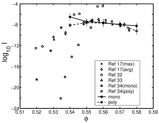
Figure 5: The logarithm of crystal nucleation rates (in units of $D_{0}/(2R)^{5}$) for different packing fractions for the polydisperse and monodisperse systems (solid lines). The experimental results as well as the results from other simulations are shown for comparison.

By analyzing the time variations of the static structure factor we were able to calculate the crystal fraction $X$, the average linear crystal size $L$ and the number density of the crystals $N_{c}$ (Fig. 4). In spite of the minuscule systems studied in the simulations, the time dependence is qualitatively similar to the experimental data. Fig. 5 shows a summary of our results both for the polydisperse case (with $5\%$ of polydispersity) and monodisperse systems together with the experimental data Harland and van Megen (1997); Schatzel and Ackerson (1993); Cheng (1998) and Monte Carlo simulations of Auer and Frenkel Auer and Frenkel (2001). The latter simulations used the umbrella sampling method in order to determine the probability of the formation of the critical size nuclei and the free-energy barrier for nucleation of a homogeneous crystal. This allowed them to get the values of the crystal nucleation rates within the framework of classical nucleation theory. Somewhat surprisingly, their results were several orders of magnitude smaller than the corresponding experimental results. In contrast, our results are in a good agreement with the experimental data. The nucleation rates for the polydisperse systems (especially for the lowest and the highest concentrations studied) confirm the well established fact that the presence of polydispersity slows the crystallization down significantly.

However, due to the small size of the systems studied in the simulations, such parameters as the average linear size and the number density of the crystals cannot be determined directly. We have found that, based on the structure factor analysis, the average crystal size of the fully crystallized system is about $0.5-0.8$ of the box size. On the other hand, the local-invariant based calculation of the number of crystallites in our systems indicates that there is only one crystallite at the end of the crystallization process.

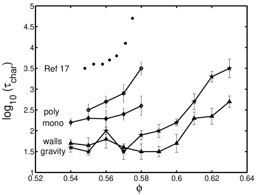
Figure 6: The logarithm of the characteristic crystallization times (measured by the crossover times - see text) in units of the diffusional characteristic times for the following cases: unbounded system(monodisperse and polydisperse cases), the system with walls and the system in the presence of gravity(monodisperse case). The experimental data from Ref. Harland and van Megen (1997) are shown.

Although we have found the crystal nucleation rates to be in a good agreement with experimental results, the characteristic times for the crystallization do not quite agree. The first difference is the absence of an induction timeHarland and van Megen (1997), defined as the time before the initialization of the crystallization. In all of the systems studied here, the crystallization starts right after the beginning of the simulation. The second difference is in the values of the crossover times. The crossover time is defined as a duration of crystallization that takes place at an approximately uniform rate. Beyond the crossover time, the crystallization rate slows down and is no longer constant. Our crossover times more than $10$ times smaller than the corresponding experimental values Harland and van Megen (1997) (see Fig. 6). To check whether this discrepancy is an artifact of the small size of the system, we ran a few simulations with $20000$ particles. The results were found to be approximately the same indicating that the size dependence is somewhat weak. Still, we observed the expected differences between the polydisperse and monodisperse systems: the crystallization processes were slower in the polydisperse systems.

V The effects of the bounding walls and the gravity

In order to investigate the dynamics of a system in the presence of the gravitational field, it is essential to first bound the system by some kind of walls. Otherwise we would deal with a free fall situation when all of the processes proceed in exactly the same way as in the absence of the gravity. Thus a good starting point is to consider the system bounded in one dimension and without any gravitational forces.

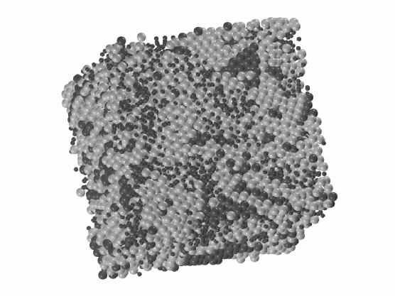
Figure 7: The snapshot of a system with volume fraction of $\phi=56\%$ and periodic boundary conditions in the middle of the crystallization process. Here, small dark, large light gray and large dark particles correspond to liquid, hcp and fcc structures respectively. The liquid particle sizes have been reduced to half their value for easier visualization.

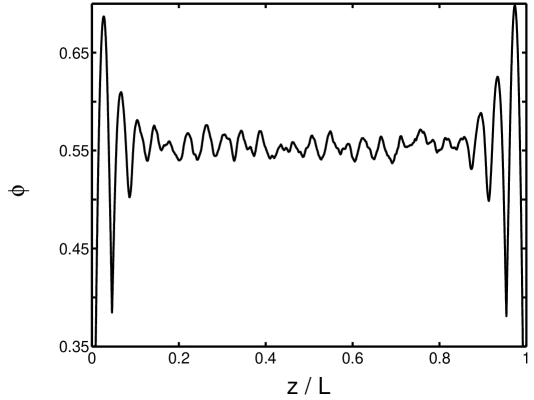
Figure 8: The density profile of a typical initial configuration of the system bounded by two walls with $\phi=55\%$. $L$ is the distance between the two walls and is equal to $21.86$ hard sphere diameters.

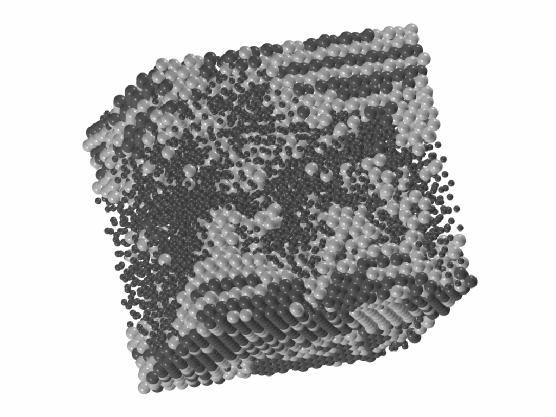
Figure 9: The snapshot of a system bounded by two walls in the middle of the crystallization process. The convention for the colors is as in Fig. 7 and again $\phi=56\%$.

The snapshot of the hard sphere configuration shown in Fig. 7 indicates the complicated nature of crystallization when periodic boundary conditions are used. Even at moderately early stages of crystallization, there is an interconnected phase of growing crystal nuclei with predominantly hcp and fcc structures. The situation is significantly simpler when walls are introduced. Even in the initial configuration (see Figure 8 for a typical example), there is pronounced layering near the flat walls. These layers lead to a heterogeneous wall-induced nucleation with growth of the crystal occurring towards the center of the channel (Figure 9). Furthermore, the crystallization is more rapid compared to the case without bounding walls, as seen in Fig. 6.

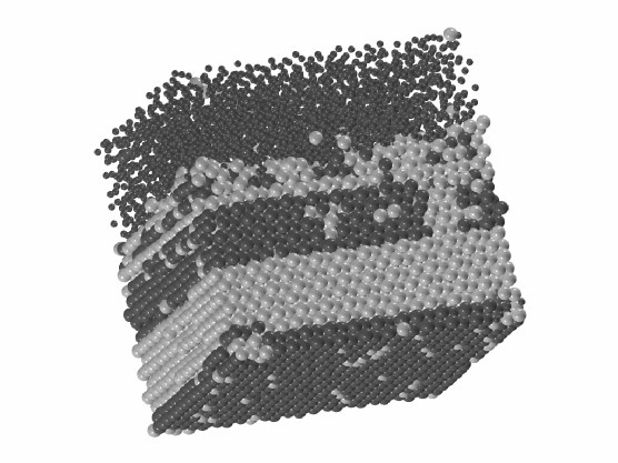
Figure 10: The snapshot of a system ($\phi=56\%$) bounded by two walls in the presence of gravity (acting downwards). The color code is as in Figure 7.

When the gravitational field in the direction perpendicular to the bounding walls is turned on, the process of crystallization switches to a different mode (see the snapshots shown in Fig. 10 and 11). The particles are seen to first settle down at the bottom of the channel, and after a while we observe a stationary phase separation with the crystal at the bottom and the liquid at the top of the channel. Note, that the crystalline region consists of almost ideal hcp crystal planes which are parallel to the bounding plane, whereas in the absence of gravity, the crystallites are stacked at random orientations.

Fig. 12 shows the variation of the concentration with the height, counting from the bottom plane. The concentration at the bottom varies from $\phi\approx 58\%$ to $\phi\approx 63\%$ exceeding the average concentration by approximately $3$-$5\%$. The concentration does not change significantly for up to half of the channel and then it comes down to $\phi\approx 43-52\%$ at the top where the system becomes a liquid. We also notice that the density profiles depend on the initial concentrations only weakly, although the higher the initial concentration of the system, the lower the propensity for the group of particles to remain liquid-like. Interestingly, for the system at $\phi=58\%$ the long time crystallization fraction is about $98\%$, although one can see from Fig. 12 that about $20\%$ of the volume of the system have concentrations which are smaller than the melting value ($54.5\%$). This can be explained as emergence of “induced” crystallization, i.e. crystallization promoted by the well-formed substrate Lin et al. (2000).

While at concentrations up to $\phi\approx 58\%$ the crystallization times for the bounded systems with and without the gravity are approximately the same, at higher concentrations we observe that the presence of gravity slows the crystallization down significantly. Thus, gravity stabilizes the glassy state by reducing the mobility of the particles even though the presence of the walls helps the crystallization. We observe crystallization in the monodisperse systems at packing fractions as high as $63\%$, which would lead to the glassy behavior in the absence of the walls.

VI The crystal structure

Finally, we have analyzed the nature of the crystal structure for all of the cases studied here. The example of the structure for one of the simulations ($\phi=56\%$, monodisperse, no walls, zero gravity) is shown in Fig. 13 as a function of time. The figure shows the percentage of the different crystal types among the particles in the crystallized regions. The hcp structure dominates in the first stages of crystallization. As the crystallization proceeds, the fcc structure emerges and starts growing. In some cases, the fcc structure reaches a value equal to $60\%$ of the crystallized volume. The bcc (and other packings) typically accounted for no larger than $5-10\%$ of the number of crystal-like hard spheres. Once the crystallization is completed, we do not observe any changes in the local structure. Our observations allow us to conclude that the fcc structure is more stable than the hcp especially because the fraction of the fcc crystals never decreases during the crystallization process Gasser et al. (2001); Bolhuis et al. (1997); Woodcock (1997).

Table 1: The values of $q_{4}(i)$, $q_{6}(i)$ and $\hat{w}_{6}(i)$ for different perfect crystal structuresten Wolde et al. (1996).

	$q_{4}$	$q_{6}$	$\hat{w}_{6}$
fcc	0.191	0.575	-0.013
hcp	0.097	0.485	-0.012
bcc	0.036	0.511	0.013
sc	0.764	0.354	0.013
icosahedral	0	0.663	-0.170

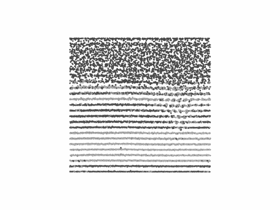
Figure 11: The snapshot of the system shown in Fig. 10 rotated so that the crystal planes are perpendicular to the image. The image sizes of the particles are greatly reduced. Note the excellent planar ordering.

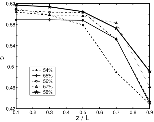
Figure 12: The concentration profile, as measured by $\phi$, for the system in the presence of the gravitational field. Here, $L$ is the distance between the two walls and is equal to $\displaystyle{\left({\pi N\over 6\phi_{total}}\right)^{1/3}}$ hard sphere diameters, where $N=10976$ is the number of particles and $\phi_{total}$ is the total concentration of the systems (shown in the legend). The accelerations due to gravity are $g_{54}\approx 4.55$, $g_{55}\approx 4.57$, $g_{56}\approx 4.60$, $g_{57}\approx 4.63$ and $g_{58}\approx 4.66$.

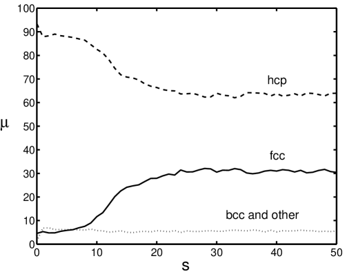
Figure 13: Plot of the fractions $\mu$ of fcc, hcp and bcc structures in the system with $\phi=56\%$ versus $s$ defined as the number of collisions (in units of $1000\times N$, where $N$ is the number of particles).