Nonlinear response of electron dynamics to a positive ion

Abstract

Electric field dynamics at a positive ion imbedded in an electron gas is considered using a semiclassical description. The dependence of the field autocorrelation function on charge number is studied for strong ion-electron coupling via MD simulation. The qualitative features for larger charge numbers are a decreasing correlation time followed by an increasing anticorrelation. Stopping power and related transport coefficients determined by the time integral of this correlation function result from the competing effects of increasing initial correlations and decreasing dynamical correlations. An interpretation of the MD results is obtained from an effective single particle model showing good agreement with the simulation results.

1 Introduction

The total electric field at a particle in a plasma determines the dominant radiative and transport properties of that particle. The properties of fields due to positive ions at a positive particle have been studied in some detail for both the static distribution of fields [1] and the dynamics of the electric field autocorrelation function [2, 3]. The latter poses a real challenge since finite charge on the site at which the field is considered precludes the use of standard linear response methods. The corresponding study of fields at a positive ion due to electrons has been considered more recently for the simplest case of a single ion of charge number $Z$ in an semiclassical electron gas. The static properties (electron charge density, electron microfield distribution) have been discussed in some detail elsewhere [4]. Here, attention is focused on the dynamics via the electric field autocorrelation function. The case of opposite sign electron fields at a positive ion is qualitatively different from same sign ion fields, since in the former case electrons are attracted to the ion leading to strong electron-ion coupling for the enhanced close configurations. It is difficult a priori to predict the qualitative features of the correlation function due to this inherent strong coupling. Consequently, the analysis here has been based on MD simulation of the correlation function followed by an attempt to model and interpret the observed results. The simulations represent classical mechanics for Coulomb interactions with the ion-electron potential modified at short distances to represent quantum diffraction effects. The details have been discussed elsewhere [4] and will not be repeated here. There are only three dimensionless parameters: the charge number of the ion, $Z$, the electron-electron coupling constant $\Gamma$, and the de Broglie wavelength relative to the interelectron distance, $\delta$. The electron-ion coupling is measured by the maximum value of the magnitude of the regularized ion-electron potential at the origin, $\sigma=Z\Gamma/\delta$. In this brief report results are reported for $\Gamma=0.1$ and $\sigma=0.25Z$, with $Z=8,20,30,$ and $40$. The corresponding density and temperature are $n=2.5\times 10^{22}$ cm^-3and $T=7.9\times 10^{5}$ $K$.

The primary observations from the simulations of the field autocorrelation function for increasing charge number are: 1) an increase in the initial value, 2) a decrease in the correlation time, and 3) an increasing anticorrelation at longer times. The stopping power for the ion by the electron gas is proportional to the time integral of the field autocorrelation function in the limit of large ion mass [5]. This same integral determines the self-diffusion and friction coefficients in this same limit [6]. The nonlinear dependence of these properties on $Z$ is therefore the result of competition between the increase of the integral due to 1) and the decrease due to 2) and 3). The results from simulation show that the latter two dynamical effects dominate the former static effect. To interpret this, a simple model for the field correlation function is proposed such that the initial correlations are given exactly, but the dynamics is determined approximately from a single electron-ion trajectory. The model reproduces well the MD simulation results and suggests an interpretation of 2) and 3).

2 MD simulation of field dynamics

The system considered consists of $N_{e}$ electrons with charge $-e$, an infinitely massive positive ion with charge $Ze$ placed at the origin, and a rigid uniform positive background for overall charge neutrality. The regularized electron-ion potential is chosen to be $V(r)=-Ze^{2}\left(1-e^{-r/\delta}\right)/r$    where $\delta=\left(2\pi\hbar^{2}/m_{e}k_{B}T\right)^{1/2}$ is the electron thermal de Broglie wavelength. For values of $r>>\delta$ the potential becomes Coulomb, while for $r<<\delta$ the Coulomb singularity is removed and $V(r)\rightarrow-Ze^{2}/\delta$. This is the simplest phenomenological form representing the short range effects of the uncertainty principle [7]. Dimensionless variables are based on scaling coordinates with the average electron-electron distance, $r_{0}$, defined in terms of the electron density $n_{e}$ by $4\pi n_{e}r_{0}^{3}/3=1$, and scaling time with the inverse electron plasma frequency. The electron electric field at the ion is obtained from the total regularized potential

$$\mathbf{E}=-\nabla_{0}V(\left\{r_{i0}\right\})=\sum_{i=1}^{N}\mathbf{e}\left(\mathbf{r}_{i0}\right)$$ (1)

where $\mathbf{r}_{i0}=\mathbf{r}_{i}-\mathbf{r}_{0}$ is the position of the $i^{th}$ electron relative to the ion, and

$$V(\left\{r_{i0}\right\})=\sum_{i=1}^{N}V(r_{i0}),\hskip 11.38092pt\mathbf{e}\left(\mathbf{r}_{i0}\right)=e\frac{\widehat{\mathbf{r}}_{i0}}{r_{i0}^{2}}(1-\left(1+\frac{r_{i0}}{\delta}\right)e^{-r_{i0}/\delta})$$ (2)

The dimensionless field autocorrelation function is defined by

$$C(t)=\frac{r_{0}^{4}}{e^{2}}<\mathbf{E}\left(t\right)\mathbf{\cdot E}>.$$ (3)

The brackets denote an average over the classical Gibbs ensemble for the composite electron-ion system at equilibrium.

Figure 1: Field autocorrelation function for $Z=8,20,30,40$ at $\Gamma=0.1$ and $\delta=0.4$.

The results for $C(t)$ from MD simulation are shown in Figure 1 for $Z=8,20,30,$ and $40$. The initial value increases approximately as a third order polynomial in $Z$ [4]. The correlation time $t_{c}$ is defined to be the time at which the correlation function first goes to zero, $C(t_{c})=0$, and is seen to decrease as $Z$ increases. Finally, in all cases there is anticorrelation ($C(t)<0$) for $t>t_{c}$. The physical basis for the increase in the initial value is easy to understand. As $Z$ increases, the electron density near the ion increases and the magnitude of the field increases for these more probable closer configurations. An explanation for the correlation time and anticorrelation is more difficult, and is the objective of the following sections. First, some consequences of this behavior are illustrated.

3 Stopping power, friction, and self-diffusion

The case of an infinitely massive ion considered here leads to exact relationships between transport coefficients characterizing three physically different phenomena: 1) the low velocity stopping power $\mathcal{S}$ for a particle injected in the electron gas, 2) the friction coefficient $\xi$ for the resistence to a particle being pulled through the gas, and 3) the self-diffusion coefficient $D$ of a particle at equilibrium with the gas. The exact relationship is [6]

$$m_{0}\xi=\left(\beta D\right)^{-1}=\mathcal{S}(v)/v=\beta Z^{2}r_{0}^{-4}\int_{0}^{\infty}dtC(t)$$ (4)

This Green-Kubo representation allows determination of these transport properties from an equilibrium MD simulation. Previous simulations of stopping power have studied the nonequilibrium state of the injected particle, measuring directly the energy degradation [8]. As discussed below, (4) provides the basis for additional interpretation of the results.

Figure 2: Stopping power $\mathcal{S}(v)/v$ for $Z=8,20,30,40$ at $\Gamma=0.1$ and $\delta=0.4$.

Figure 2 shows the dimensionless stopping power obtained from the results of Figure 1 as a function of $Z$. Also shown is the Born approximation $\propto Z^{2}$, valid for small $Z$. Previous simulations [8] and some experiments [9] suggest a crossover at larger $Z$ to a weaker growth $\propto Z^{2}$. The data in Figure 2 has been fit to a such a crossover function showing consistency with these earlier results. This behavior is somewhat puzzling in light of the strong growth of the initial value $C(0)\approx Z^{3}$ at large $Z$. Making this explicit, the stopping power can be expressed as

$$\mathcal{S}(v)/v\propto Z^{5}\int_{0}^{\infty}dtf(t),\hskip 36.135ptf(t)=C(t)/C(0)$$ (5)

Evidently, the dynamical effects of the normalized correlation function $f(t)$ decrease the stopping power as $\sim Z^{-3.5}$ for large $Z$. A possible explanation for this is given in the following section.

4 Single particle dynamics

Consider again the initial covariance $C(0)$ for which three representations can be given

$$C(0) = \frac{3}{4\pi}\int d\mathbf{re}\left(\mathbf{r}\right)\mathbf{\cdot}\left[g_{ie}(r)\mathbf{e}\left(\mathbf{r}\right)+\frac{3}{4\pi}\int d\mathbf{r}^{\prime}g_{ie}(\mathbf{r},\mathbf{r}^{\prime})\mathbf{e}\left(\mathbf{r}^{\prime}\right)\right]$$ (6)

$$= \frac{3}{4\pi Z\Gamma}\int d\mathbf{r}g_{ie}(r)\nabla\mathbf{\cdot e}\left(\mathbf{r}\right)$$

$$= \frac{3}{4\pi}\int d\mathbf{r}g_{ie}(r)\mathbf{e}_{mf}\left(\mathbf{r}\right)\mathbf{\cdot e}\left(\mathbf{r}\right)$$

The first equality expresses the covariance in terms of the one and two electron correlations with the ion, $g_{ie}(r)$ and $g_{ie}(\mathbf{r},\mathbf{r}^{\prime})$ respectively. The second equality exploits the relationship for the field to the Gibbs factor $\beta U(\left\{r_{i0}\right\})=Z\Gamma V(\left\{r_{i0}\right\})$ and an integration by parts. This second representation requires only the one electron correlation function. The third representation is obtained from the second by an integration by parts to identify the mean force field $\mathbf{e}_{mf}\left(\mathbf{r}\right)=\nabla\ln g_{ie}(r)$. The third equality of (6) is similar to the first with apparent neglect of the two electron-ion correlations. However, these latter contributions are incorporated exactly in the mean force field $\mathbf{e}_{mf}\left(\mathbf{r}\right)$. This suggests a corresponding model for finite times

$$C(t)\rightarrow\frac{3}{4\pi}\int d\mathbf{v}d\mathbf{r}\phi(v)g_{ie}(r)\mathbf{e}_{mf}\left(\mathbf{r}\right)\mathbf{\cdot e}\left(\mathbf{r}(t)\right)$$ (7)

where $\phi(v)$ is the normalized Maxwellian and $\mathbf{r}(t)$ is a single electron trajectory in the presence of the ion, generated by the potential associated with $g_{ie}(r)$ for stationarity. Further details and a justification based on the Vlasov equation will be given elsewhere. Clearly, the initial covariance is given exactly by this approximation. For practical purposes $g_{ie}(r)$ and the associated field and potential are represented here by the non-linear Debye-Huckel approximation with effective charge number and screening length adjusted to fit the MD data.

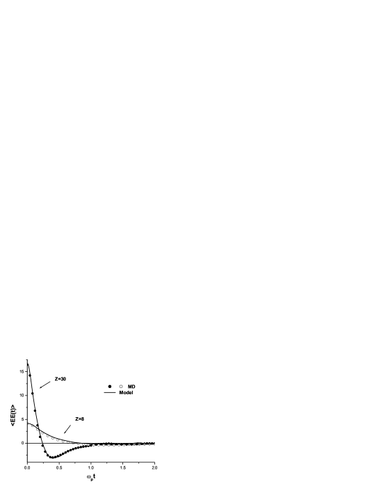
Figure 3: Comparison of $C(t)$ from MD and from Eq.7 for $Z=8$ and $30$ at $\Gamma=0.1$ and $\delta=0.4$.

Figure 3 shows a comparison of (7) with the MD results of Fig. 1 for $Z=8$ and $Z=30$. The agreement is very good, indicating that the dominant $Z$ dependence is captured by the initial correlations and the single particle dynamics.

5 Discussion

The good agreement of the simple model in the previous section suggests that the decrease in correlation time and build up of anticorrelation can be understood in terms of one electron dynamics. As $Z$ increases the probability of close electron ion configurations increase. The electron is subjected to greater acceleration toward the ion and the time to reverse its sign decreases. This is the effect of decreasing correlation time. Once the field has reversed sign there is anticorrelation. Since the closer configurations imply larger field values the magnitude of this anticorrelation also increases with increasing $Z$. It remains to quantify this picture but the single electron dynamics appear to provide qualitative confirmation. A more complete discussion will be provided elsewhere.

6 Acknowledgments

Support for this research has been provided by the U.S. Department of Energy Grant No. DE-FG03-98DP00218. J. Dufty is grateful for the support and hospitality of the University of Provence.

References

- [1] Dufty J W in Strongly Coupled Plasmas, 493, de Witt H and Rogers F editors (NATO ASI Series, Plenum, NY, 1987).
- [2] Boercker D, Iglesias C, and Dufty J W 1987 Phys. Rev. A 36, 2254
- [3] Berkovsky M, Dufty J W, Calisti A, Stamm R, and Talin B 1996 Phys. Rev. E 54, 4087-4097.
- [4] Talin B, Calisti A and Dufty J W 2002 Phys. Rev. E 65, 056406
- [5] Dufty J W and Berkovsky M 1995 Nucl. Inst. Meth. B 96 626
- [6] Dufty J W and Berkovsky M in Physics of Strongly Coupled Plasmas edited by Kraeft W, Schlanges M, Haberland H and Bornath T (World Scientific, River Edge, NJ, 1996)
- [7] Minoo H, Gombert M and Deutsch C 1981 Phys. Rev. A 23 924
- [8] Zwicknagel G, Toepffer C and Reinhard P-G 1999 Physics Reports 309 118
- [9] Winkler Th. et al. 1997 Nucl. Inst. and Meth. A 391 12