Asymmetric binaries and hierarchy of states in self-gravitating systems

Abstract

We complete the analysis of the equilibrium shapes of rotating self-gravitating gases initiated in Phys. Rev. Lett. 89 031101 (2002) by studying the formation and thermodynamics of asymmetric binaries and by introducing a family of order parameters to classify the possible equilibrium states.

Gravity-dominated systems such as classical self-gravitating gases are known to possess highly non-standard thermodynamic properties binney&tremaine87 ; padmanabhan90 ; padmata . The long-range nature of the Newtonian potential prevents thermodynamic functionals from being extensive gallavotti99 , causing such features as the inequivalence of statistical ensembles, the occurrence of negative specific heats and of collapse transitions, and the existence inhomogeneous ground states lyndenbell67 ; lyndenbell68 ; thirring70 ; devega96 ; chavanis01 . These attributes are not peculiar to gravitating gases alone. Similar traits mark the behaviour of systems with long-range, non-integrable potentials barre01 , of finite systems or of systems of a size comparable to the interaction range, such as atomic clusters or highly excited (“hot”) nuclei gross82 ; gross140 , are even present in certain short-ranged models compagner and in general at phase separations gross174 . Besides the relevance to astrophysics and cosmology strictly speaking, understanding the equilibrium state of self-gravitating systems is hence important also from a broader, fundamental viewpoint gross174 .

In a recent work prl ; epjb , to be later referred to as I, we investigated the possible equilibrium shapes of three-dimensional rotating self-gravitating gases using a microcanonical mean-field theory in which the system is enclosed in a finite spherical volume $V$ with the total energy $E$ and the total angular momentum $\boldsymbol{L}$ conserved. The singularity of the Newtonian potential at short distances was cured by the use of Lynden-Bell statistics lyndenbell67 . It turned out that, along with the known “gaseous” and “collapsed” (a single, dense cluster) states, the system can form symmetric “binaries” (two identical clusters) if $E$ is sufficiently low, that is if gravity is strong enough, and rotation is sufficiently fast. Moreover, at intermediate $E$ and $\boldsymbol{L}$, a large phase-coexistence region with negative specific heat appears, where the system is found in dense structures (either a single cluster or a binary) embedded in a vapor.

The purpose of this paper is to complete the study of I by describing the formation and thermodynamics of asymmetric binaries (which are far more common in the universe than symmetric ones). Furthermore, a family of order parameters will be introduced to discern the possible equilibria and allow for a classification of the equilibrium states. Some “exotic” equilibria (with a very low entropy) that can be obtained using these order parameters are presented as an example.

We begin by recalling the key steps in the theory of I. The Hamiltonian is ($i,j=1,\ldots,N$)

$$H=\frac{1}{2m}\sum_{i}p_{i}^{2}-Gm^{2}\sum_{i<j}|\boldsymbol{r}_{i}-\boldsymbol{r}_{j}|^{-1}$$ (1)

with $\boldsymbol{r}_{i}\in V\subset\mathbb{R}^{3}$ denoting the position and $\boldsymbol{p}_{i}\in\mathbb{R}^{3}$ the momentum of the $i$-th particle, $m$ being its mass. $G$ is the gravitational constant. The task is to find the particle density profiles that maximize the Boltzmann entropy $S=k\log W$, where the state sum $W$ is given by

$$W=\frac{\alpha}{N!}\int\delta(H-E)~{}\delta(\boldsymbol{L}-\sum_{i}\boldsymbol{r}_{i}\times\boldsymbol{p}_{i})~{}d^{3N}\boldsymbol{r}~{}d^{3N}\boldsymbol{p}$$ (2)

with $\alpha$ a constant. $W$ is a function of $E$ and $\boldsymbol{L}$, as are $S$ and the desired density profiles. The radius $R$ of the box is taken to be fixed. Adhering to the notation of I, we shift to the reduced variable $\boldsymbol{x}=\boldsymbol{r}/R$, which we shall indicate as $\boldsymbol{x}=(x_{1},x_{2},x_{3})$ (Cartesian representation) or $\boldsymbol{x}=(x,\theta,\phi)$ (spherical representation). Particles are assumed to have “hard cores”, so that the density profile $c$ is normalized as $\int c(\boldsymbol{x})d\boldsymbol{x}=\Theta$, with $0\leq c\leq 1$. $\Theta$ is a fixed parameter ($0\leq\Theta\leq 4\pi/3$) which throughout this study, as in I, is taken to be $\Theta=0.02$. A brief discussion about the dependence of the results on $\Theta$ is given at the end of the paper. Finally, we take $m=1$ and measure energy and angular momentum in units of $GN^{2}/R$ and $\sqrt{RGN^{3}}$, respectively.

Assuming Lynden-Bell statistics to mimic the hard cores lyndenbell67 , at stationary points of the entropy surface the density profile $c$ satisfies the condition (see I for details)

$$\log\frac{c(\boldsymbol{x})}{1-c(\boldsymbol{x})}=\frac{\beta}{\Theta}\int\frac{c(\boldsymbol{x^{\prime}})}{|\boldsymbol{x}-\boldsymbol{x^{\prime}}|}~{}d\boldsymbol{x^{\prime}}+\frac{1}{2}\beta(\boldsymbol{\omega}\times\boldsymbol{x})^{2}-\mu$$ (3)

where

$$\beta=\frac{3/2}{[E-\frac{1}{2}\boldsymbol{L}^{T}\mathbb{I}^{-1}\boldsymbol{L}-\Phi[c]]}~{},$$ (4)

$\boldsymbol{\omega}=\mathbb{I}^{-1}\boldsymbol{L}$ is the angular velocity, and $\mu$ is a Lagrange multiplier implementing the constraint on $\Theta$. $\mathbb{I}$ stands for the inertia tensor, with elements ($a,b=1,2,3$)

$$I_{ab}[c]=\frac{1}{\Theta}\int c(\boldsymbol{x})(x^{2}\delta_{ab}-x_{a}x_{b})d\boldsymbol{x}$$ (5)

(in units of $NR^{2}$), while $\Phi$ is the gravitational potential. In general, the solutions of Eq. (3), whose number and form depend on $E$ and $\boldsymbol{L}$, can be written in spherical coordinates as

$$c(\boldsymbol{x})=\sum_{l=0}^{\infty}\sum_{m=-l}^{l}b_{lm}(x)Y_{lm}(\theta,\phi)$$ (6)

where the “weights” $b_{lm}(x)$ have to be determined by solving (numerically) the system of integral equations

$$b_{lm}(x)=\int g(x,\theta,\phi)Y_{lm}(\theta,\phi)~{}d\cos\theta~{}d\phi$$ (7)

$$g(x,\theta,\phi)=\left[1+e^{\frac{\beta}{\Theta}\sum_{l,m}u_{lm}(x)Y_{lm}(\theta,\phi)-\frac{1}{2}\beta\omega^{2}x^{2}\sin^{2}\theta+\mu}\right]^{-1}$$

Some details of this task are discussed in I.

If $\boldsymbol{L}$ is taken to lie along the $3$-axis and if only even harmonics ($l=0,2,4,\ldots$) are included in the series (6), entropy-maximizing solutions of (3) can be divided in two main classes (see I): (a) axial-rotationally symmetric ones, e.g. gas-cloud (high $E$, low $L$), distorted gas clouds or disks (high $E$, high $L$), and single clusters (low $E$, low $L$); (b) axial-rotationally asymmetric ones, like identical double clusters or symmetric binaries (SBs, low $E$, high $L$). The former are independent of the $\phi$ angle, and thus for them the series (6) involves only the zonal harmonics, with $m=0$. The latter, instead, must depend on $\phi$ and the lowest-order term in (6) that can provide this dependence is the sectoral harmonics $Y_{2,2}$. In fact, on physical grounds, SBs can be characterized by a non-zero value of the order parameter

$$D_{2,2}=\left|\int x^{4}~{}b_{2,2}(x)dx\right|$$ (8)

which is proportional to the difference between the diagonal components of the inertia tensor in the $1$ and $2$ directions. Using (5) and (6) it is indeed easy to see that

$$D_{2,2}=\Theta\sqrt{\frac{15}{16\pi}}~{}|I_{11}-I_{22}|$$ (9)

The inclusion of odd harmonics leads to new solutions, namely asymmetric binaries (ABs). A sample of asymmetric binaries obtained in this way (with the addition of fixing the center of mass at $\boldsymbol{x}=\boldsymbol{0}$) is shown in Fig. 1.

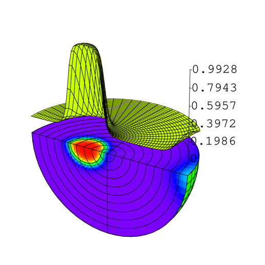
(a) $E=-0.60$, $L=0.46$

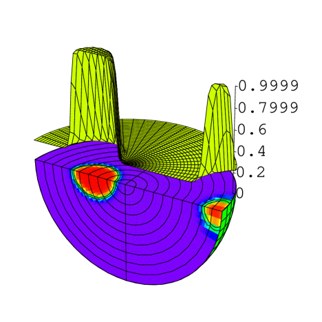
(b) $E=-1.16$, $L=0.46$

Figure 1: Two asymmetric binaries obtained from Eq. (3). The contour plot is shown together with the density profile. (a) Incipient binary, with a broad low-density body detached from the central cluster. (b) Well-formed binary (very low energy).

As it was to be expected, such solutions appear at low energies at intermediate angular momenta ($L\simeq 0.46$) and exist in a small range of values of $L$ up to $L\simeq 0.5$. This whole region lies in the mixed phase with negative specific heat of I, hence asymmetric binaries at equilibrium are embedded in a vapor and they don’t exist as a “pure” phase. Moreover, in this range they are significantly more probable than symmetric binaries, as shown in Fig. 2, where the entropy of the different stable solutions at $L=0.46$ is shown.

Figure 2: Entropy of the different stable solutions of Eq. (3) at $L=0.46$. The quantity $4E$ has been subtracted from the entropy to make the separation and the curvature more evident.

A simple physical argument suffices to explain why at high angular momenta ABs must have a much lower entropy than SBs, if they exist at all. SBs have a larger moment of inertia than ABs, hence a smaller rotational energy. As a consequence, for SBs the “random” kinetic contribution $E-L^{2}/(2I)$ is larger than for ABs. Thus they have a larger entropy. So ABs are expected to be strongly suppressed or significantly less probable at high angular momenta. Indeed, we were unable to find stable asymmetric binaries for $L>0.5$. The fact that ABs tend to form the smaller cluster in proximity of the boundary of the box is due to the fact that ABs start to form by evaporating small masses from a large, dense cluster. The conservation of the center of mass relegates them to the border. In well formed binaries, the peak of density in the smaller cluster is separated from the boundary.

In Fig. 3 the caloric curve $\beta=\partial S/\partial E$ versus $E$ is shown at $L=0.46$.

Figure 3: Caloric curve $\beta$ vs $E$ at $L=0.46$. Notice that the curvature of the entropy surface as a function of $E$ and $L$, i.e. $S_{EE}S_{LL}-S_{EL}^{2}$, is negative along the $AB$ branch.

The jump occurring at $E=-0.2$, where ABs become more favorable than SBs, is an artifact of the asymptotics employed in the mean-field theory of I. (Being $S$ a smooth and multiply-differentiable function, such a feature is clearly spurious.)

Again on physical grounds, the natural order parameter for AB solutions is $\left\langle{x_{1}^{3}}\right\rangle:=\int x_{1}^{3}~{}c(\boldsymbol{x})d\boldsymbol{x}$, because in spatially asymmetric structures it must be non-zero because of evident symmetry reasons (the two clusters are aligned along the $x_{1}$ axis), at odds with what must happen in symmetric structures. Now using (6) one can see by working out explicitly the integrals involving spherical harmonics morse that

$$\left\langle{x_{1}^{3}}\right\rangle=\sqrt{\frac{12\pi}{25}}\int x^{5}b_{1,1}(x)dx-\sqrt{\frac{6\pi}{175}}\int x^{5}b_{3,1}(x)dx+\\ +\sqrt{\frac{2\pi}{35}}\int x^{5}b_{3,3}(x)dx$$ (10)

In principle, all of the above terms should be considered. However, in any spatially symmetric structure (gas, single cluster, SBs) all of them are zero, because odd harmonics do not contribute, as discussed above. Each of them is non-zero only in presence of spatial asymmetries, as in ABs, hence any of them can be used as an order parameter. In particular, we find it convenient to choose the quantity

$$D_{3,1}=\left|\int x^{5}~{}b_{3,1}(x)dx\right|$$ (11)

whose behaviour at $L=0.46$ is shown in Fig. 4. AB solutions appear at $E=-0.18$, where the order parameter jumps discontinuously from zero to a finite value, and becomes more favorable than SBs at $E=-0.2$.

Figure 4: Behaviour of the order parameter for asymmetric binaries $D_{3,1}$ as a function of energy at $L=0.46$.

Eq.s (8) and (11) suggest that, in general, one can classify the different equilibrium states by introducing the family of order parameters defined by

$$D_{l,m}=\left|\int x^{l+2}b_{l,m}(x)dx\right|$$ (12)

with integers $l=0,1,2,\ldots$ and $m=-l,-l+1,\ldots,l$. For small $l$, each of these functions has a simple physical interpretation.

For $l=0$, $D_{0,0}$ is simply a constant proportional to $\Theta$, since, recalling that $\int c(\boldsymbol{x})d\boldsymbol{x}\equiv\left\langle{1}\right\rangle=\Theta$,

$$\int c(\boldsymbol{x})d\boldsymbol{x}=2\sqrt{\pi}\int x^{2}b_{0,0}(x)dx$$ (13)

For $l=1$, one has that $D_{1,1}$, $D_{1,0}$ and $D_{1,-1}$ are nothing but the coordinates of the center of mass (modulo a proportionality constant):

$$x_{1}^{CM}\equiv\left\langle{x_{1}}\right\rangle=\sqrt{\frac{4\pi}{3}}\int x^{3}b_{1,1}(x)dx$$

$$x_{2}^{CM}\equiv\left\langle{x_{2}}\right\rangle=\sqrt{\frac{4\pi}{3}}\int x^{3}b_{1,-1}(x)dx$$ (14)

$$x_{3}^{CM}\equiv\left\langle{x_{3}}\right\rangle=\sqrt{\frac{4\pi}{3}}\int x^{3}b_{1,0}(x)dx$$

For $l=2$, the situation is slightly more involved. $D_{2,0}$ can be easily seen to be linked to the quantity

$$\left\langle{x^{2}-3x_{3}^{2}}\right\rangle=-\sqrt{\frac{16\pi}{5}}\int x^{4}b_{2,0}(x)dx$$ (15)

which is a convenient order parameter for disk (deformed gas) solutions. In fact, for an hypothetical configuration being a perfect sphere (say a homogeneous gas cloud filling the whole $V$), one would have $D_{2,0}=0$ evidently. When rotation deforms the cloud by shrinking it along the $3$-axis, one would have $D_{2,0}\neq 0$. As discussed in I, $D_{2,2}$ is instead the order parameter discerning axial-rotationally symmetric structures from axial-rotationally asymmetric ones (it is non zero for both SBs and ABs). It is particularly convenient for SBs because of its connection to the inertia tensor components, see (9). As for the remaining $D_{2,m}$’s, they can be easily seen to be related to the off-diagonal components of the inertia tensor (5).

It is clear that higher-order $D$’s are all connected to homogeneous polynomials in $x_{1}$, $x_{2}$, $x_{3}$, which are in turn connected to the Cartesian representation of spherical harmonics morse . For example, for $l=3$, $D_{3,0}$ is connected to

$$\left\langle{2x_{3}^{3}-3x_{1}^{2}x_{3}-3x_{2}^{2}x_{3}}\right\rangle=\sqrt{\frac{16\pi}{7}}\int x^{5}b_{3,0}(x)dx$$ (16)

Their physical interpretation for larger $l$ is however less straightforward.

Using these order parameters, solutions can be classified hierarchically, a procedure that is particularly effective at high $L$. In our setting, with the center of mass fixed at $\boldsymbol{x}=\boldsymbol{0}$ one has the following picture. Homogeneous gas clouds have all $D_{lm}$’s equal to zero except $D_{0,0}$. For deformed clouds (disks) only $D_{l,0}$ with $l$ even are non zero. For symmetric binaries (which are connected to “gas”-like solutions continuously, see I), also $D_{2,2}\neq 0$ (and in general all $D_{l,m}$ with $l$ and $m$ even), all other $D$’s being zero, while for asymmetric binaries $D_{3,1}$ is also not zero. This classification can be continued further, for the order parameters (4) allow to construct all possible solutions of (3), by adding a proper field that selects the solution for which the chosen order parameter is not zero. As an example, we show in Fig. 5 two of several equilibria that can be obtained in this way at very high angular momentum. Of course, such “exotic” solutions of (3), if stable, have much lower entropy than those discussed in I and here.

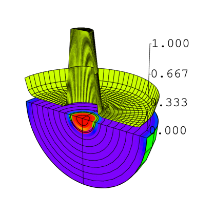
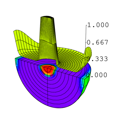
Figure 5: Two “exotic” solutions of (3) obtained via the order parameters (12). (a) Single cluster surrounded by a ring. (b) Single cluster with two “satellites”. These solutions coexist at $E=-0.5$ and $L=0.7$.

To summarize, we have carried further the equilibrium study of rotating self-gravitating gases of classical non-overlapping particles started in I by describing the formation and thermodynamics of asymmetric binaries. Moreover, we introduced a family of order parameters that allow to characterize all the different shapes that can be encountered (homogeneous gas, disk, symmetric binary, asymmetric binary, along with more exotic states), and discussed their physical meaning in simple cases. The present study does not substantially alter the global phase diagram presented in I, since asymmetric binaries do not exist as a pure thermodynamic state but only in the phase coexistence region. Among the problems that remain open we would like to mention the following two. First, the dependence on $\Theta$. Our results have been obtained at fixed $\Theta=0.02$. Different $\Theta$’s may lead to different results. By letting $\Theta\to 0$ one obtains the case of overlapping particles (hard cores are neglected and Lynden-Bell statistics is replaced by Boltzmann statistics in space), which is a classical problem in cosmology dating back to antonov62 . The rotating case is dealt with in npb . For Boltzmann particles we haven’t found any evidence of asymmetric binaries. On the other hand, when $\Theta$ grows ($\Theta\leq 4\pi/3$) the system may become too closely packed and the interesting features one observes for small $\Theta$ might disappear at some point. The second problem is the dependence on $R$. Throughout this paper we have assumed that $R$ is fixed but it would be interesting to analyze this problem in a context in which $R$ varies, for instance to mimic an expanding-universe scenario.

References

- (1) J. Binney and S. Tremaine. Galactic dynamics. Princeton University Press (Princeton, NJ), 1987.
- (2) T. Padmanabhan. Phys. Rep. 188 286 (1990)
- (3) T. Padmanabhan. Theoretical astrophysics I. Cambridge University Press (Cambridge, UK), 2000.
- (4) G. Gallavotti. Statistical mechanics. Springer (Berlin), 1999.
- (5) D. Lynden-Bell. Mon. Not. R. Astron. Soc. 136 101 (1967)
- (6) D. Lynden-Bell and R. Wood. Mon. Not. R. Astron. Soc. 138 495 (1968)
- (7) W. Thirring. Z. Phys. 235 339 (1970)
- (8) H.J. de Vega, N. Sanchez, and F. Combes. Nature (London) 383 66 (1996)
- (9) P.H. Chavanis, C. Rosier, and C. Sire. Preprint cond–mat/0107345.
- (10) J. Barre, D. Mukamel and S. Ruffo. Phys. Rev. Lett. 87 030601 (2001). Preprint cond-mat/0102036.
- (11) D.H.E. Gross and H. Massmann. Nucl. Phys. A 471 339c (1987)
- (12) P.A. Hervieux and D.H.E. Gross. Z. Phys. D 33 295 (1995)
- (13) A. Compagner, C. Bruin and A. Roelse. Phys. Rev. A 39 5989 (1989)
- (14) D.H.E. Gross. Microcanonical thermodynamics. World Scientific (Singapore), 2001.
- (15) E.V. Votyakov, H.I. Hidmi, A. De Martino and D.H.E. Gross. Phys. Rev. Lett. 89 031101 (2002). Preprint cond-mat/0202140.
- (16) E.V. Votyakov, A. De Martino and D.H.E. Gross. Eur. Phys. J. B 29 593 (2002). Preprint cond-mat/0207153.
- (17) P.M. Morse and H. Feshbach. Methods of theoretical physics, Chapter 10. McGraw-Hill (New York), 1953.
- (18) V.A. Antonov. Vest. Leningrad Univ. 7 135 (1962)
- (19) A. De Martino, E.V. Votyakov and D.H.E. Gross. Preprint cond-mat/0208230 (submitted).