Abstract

Single electron transistors (SETs) are very sensitive electrometers and they can be used in a range of applications. In this paper we give an introduction to the SET and present a full quantum mechanical calculation of how noise is generated in the SET over the full frequency range, including a new formula for the quantum current noise. The calculation agrees well with the shot noise result in the low frequency limit, and with the Nyquist noise in the high frequency limit. We discuss how the SET and in particular the radio-frequency SET can be used to read out charge based qubits such as the single Cooper pair box. We also discuss the backaction which the SET will have on the qubit. The back action is determined by the spectral power of voltage fluctuations on the SET island. We will mainly treat the normal state SET but many of the results are also valid for superconducting SETs.

1 Introduction

The single-electron transistor (SET) is known as a highly sensitive electrometer [1, 2] based on the Coulomb blockade [3, 4]. Electrons tunnel one by one through two small-capacitance tunnel junctions, with capacitances $C_{L}$ and $C_{R}$. The gate, with capacitance $C_{g}$, is used to modulate the generated current, and the island is also capacitively coupled to the system to be measured through $C_{c}$. The charging energy $E_{C}=e^{2}/2C_{\Sigma}$, $C_{\Sigma}=C_{L}+C_{R}+C_{g}+C_{c}$, associated with a single electron prevents sequential tunneling through the island at voltages below a threshold $V_{t}$, which can be controlled by applying a voltage $V_{g}$ to the gate. This Coulomb blockade is effective at temperatures $T<E_{C}/k_{B}$ and for junction resistances larger than the resistance quantum $R_{K}=h/e^{2}\approx 25.8\mathrm{k\Omega}$.

SETs can be made using several different technologies, for example they can be fabricated from metallic (often aluminum based) systems, from quantum dots in GaAs and silicon, or from carbon nanotubes.

Often the SETs are operated at low temperatures, however room temperature operation has been demonstrated in several cases[5, 6, 7].

Both the ultimate sensitivity and the back action of SET during measurement is determined by the noise in the SET. By understanding the noise in the SET we can optimize the use of the SET for each application.

1.1 RF-SET

The conventional SET, based on measuring either the current or voltage across the transistor, has suffered from the relatively large output resistance R of the transistor. For the typical resistance values of $100\,\mathrm{k\Omega}$ and cable capacitance of $C\sim 1\mathrm{nF}$, the corresponding RC time limits the bandwidth to a few kHz.

With the invention of the radio-frequency SET (RF-SET)[8] the SET was made fast and very sensitive. By connecting the SET very close to a cold amplifier the upper frequency limit was improved to about 1 MHz[9, 10]. With the invention of the RF-SET[8] frequencies above 100 MHz could be reached.

The operation principle of the RF-SET is similar to that of a radar. A weak RF-signal (the carrier) is launched via a directional coupler and a bias tee, towards the tank circuit in which the SET is embedded. The reflected signal depends critically on the dissipation in the tankcircuit, and thus in the SET. This means that the carrier is modulated by the gate signal. The reflected signal is amplified by a cold amplifier and a number warm amplifiers. The reflected signal can be analyzed either in the frequency domain or in the time domain. Typical carrier frequencies are in the range of 0.3-2 GHz.

Charge sensitivities of $1.2\cdot 10^{-5}$ and $3.2\cdot 10^{-6}$ $e/\sqrt{\mathrm{Hz}}$ have been reached for signal frequencies of 100 and 2 MHz, respectively[8, 11]. The RF-SET can be used as a readout device in applications from very sensitive charge meters and current standards[4] in which electrons are counted or pumped one by one, to read out of quantum bits[12, 13, 14, 15] or to work as photon detectors [16].

2 SET - orthodox theory

Consider a small metallic SET island coupled via low transparency tunnel barriers to two external leads, and coupled capacitively to an object to be measured. In Fig. 1 we have used the example of a Single Cooper-pair Box (SCB)[17] which may serve as a qubit in a quantum computer. The SCB is controlled by a voltage source $V^{qb}_{g}$.

Figure 1.  : Schematic figure of the SET capacitively coupled to a Single Cooper-pair Box (SCB).

Following orthodox SET theory[2, 3] we use the integer number of electrons on the SET island ($N$) as a basis for describing its dynamics. This is motivated by the low transparency junctions. The charge on the island is the sum of the electrons, the background charge, and the charge induced by the the voltages on the three island capacitances. Electrostatics gives for the Coulomb charging energy $E_{ch}$ and island potential $V_{I}$:

$$E_{ch}(N) = E_{C}(N-n_{x})^{2},\ \ E_{C}=\frac{e^{2}}{2C_{\Sigma}},$$

$$V_{I}(N) = \alpha_{L}V-\frac{e(N-n_{x})}{C_{\Sigma}},\ \ \alpha_{L}=\frac{C_{R}}{C_{\Sigma}},\ \ \alpha_{R}=\frac{C_{L}}{C_{\Sigma}},$$ (1)

where $n_{x}e=V_{g}^{qb}C_{g}^{qb}$ is the charge induced on the gate capacitance $C_{g}^{qb}$ by the external voltage source $V_{g}^{qb}$. $\alpha_{L/R}$ describes the capacitive voltage division over the $L/R$ junction, were we have neglected the small gate and coupling capacitances $\{C_{c},C_{g}\}\ll\{C_{L},C_{R}\}$.

The orthodox theory neglects mainly three things: the effect of the electromagnetic environment of the SET [18], higher order tunneling processes, i.e. cotunneling [19], and that for high frequency dynamics the transition rates are frequency dependent. As long as the electromagnetic environment has a low impedance compared to the quantum resistance $R_{Q}=h/4e^{2}\approx 6.45\mathrm{k\Omega}$ (which is often the case for SETs) the corrections due to the environment are small. The same is true for the cotunneling corrections as long as the resistance of the SET is large compared to $R_{Q}$. To take into account the frequency dependence of the transition rates, including the energy exchange with the measured system, is the main objective of the quantum theory presented in section 3.2.

2.1 Transition rates

The dynamics of the SET consists of stochastic transitions between the charge states, i.e. by electrons randomly tunneling on and off the island. In orthodox SET theory the rates for the different transitions are given by the Golden Rule rates for tunneling through the left and right tunnel junctions

$$\Gamma^{L/R}(E_{if})=\frac{R_{K}}{R^{L/R}_{T}}\frac{E_{if}}{h}\frac{1}{1-e^{-E_{if}/k_{B}T}},$$ (2)

where $E_{if}$ is the energy difference between the initial and final state and the Bose function appears from the convolution of the two Fermi functions for the filled initial states and the empty final states in the leads. $E_{if}$ has two terms; one is the change in charging energy, and the other is the work done by the voltage bias.

To be specific we now consider the electrons to gain energy from the voltage source by tunneling from left to right. Then the rates $\Gamma_{n\pm}^{L/R}$ for transitions from charge state $n$ to $n\pm 1$ across the left/right junction are

$$\begin{array}[]{cc}\Gamma_{n+}^{L}=\Gamma^{L}(E_{n(n+1)}+eV_{L}),&\Gamma_{n+}^{R}=\Gamma^{R}(E_{n(n+1)}-eV_{R}),\\ \Gamma_{n-}^{L}=\Gamma^{L}(E_{n(n-1)}-eV_{L}),&\Gamma_{n-}^{R}=\Gamma^{R}(E_{n(n-1)}+eV_{R}),\end{array}$$ (3)

where $E_{mn}=E_{ch}(m)-E_{ch}(n)$ and $V_{L/R}=\alpha_{L/R}V$ is the voltage drop over the $L/R$ junction. We denote the sum of rates taking the SET island from $n$ to $n\pm 1$ with $\Sigma_{n\pm}=\Gamma_{n\pm}^{L}+\Gamma_{n\pm}^{R}$.

2.2 Master equation and steady-state

During a specific measurement, i.e. a realisation of the stochastic process, the number of (extra) electrons on the SET island as a function of time is piecewise constant, with steplike changes due to instantaneous tunnel events (see Fig. 2a-b). Mathematically one may describe the dynamics of this process averaged over a large number of measurements. Introducing the probability $P_{n}(t)$ of finding the SET in charge state $n$ at time $t$ we may write down a master equation

$$\partial_{t}\bar{P}(t)=\hat{\Sigma}\cdot\bar{P}(t),$$ (4)

where $\bar{P}=[\dots P_{-1}(t)\ P_{0}(t)\ P_{1}(t)\dots]^{T}$ is a column vector and $\hat{\Sigma}$ is the tridiagonal transition rate matrix with off-diagonal elements $(\hat{\Sigma})_{(n\pm 1)n}=\Sigma_{n\pm}$, and to ensure probability conservation $(\hat{\Sigma})_{nn}=-(\Sigma_{n+}+\Sigma_{n-})$. The solution to Eq. (4) may be written $\bar{P}(t)=\hat{\Pi}(t)\cdot\bar{P}(0)$, introducing the time-evolution operator (matrix) $\hat{\Pi}(t)=e^{\hat{\Sigma}t}$. To compute the matrix exponent one needs to diagonalize $\hat{\Sigma}$. The steady-state corresponds to the eigenvector of $\hat{\Sigma}$ with eigenvalue zero, and the other eigenvalues determine rates for exponential decay of the corresponding eigenvector.

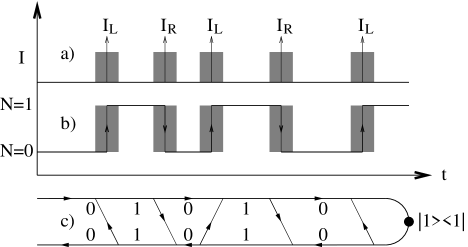
Figure 2.  : In orthodox theory the transitions between charge states in the SET are considered to be instantaneous. For a specific realisation (measurement) this results in: a) The currents through the left/right junctions $I_{L}/I_{R}$ consist of a train of delta-peaks. b) The charge on the island $N(t)$ is a telegraph signal. In order to calculate the transition rates one uses the Golden Rule approximation, which includes integration over a timescale of $h/E_{if}$, where $E_{if}$ is the energy gain in the transition. This is indicated as grey areas in figures a) and b). c) In the real-time Keldysh formalism this timescale of tunneling reappears as a timescale on which the density matrix is off-diagonal.

Figure 3.  : When an electron tunnels from/to the leads to/from the island the charges on the capacitances will redistribute. The charge transport across the boundary of a region containing the SET island plus its nearby capacitances is shown for a) an electron tunneling onto the island from the left lead, and b) an electron tunneling from the island into the right lead. $e\alpha_{L/R}$ represents a displacement charge.

2.3 Charge, Voltage and Current

In order to calculate physical quantities we introduce operators for the number of (excess) electrons on the island ($\hat{N}$) and the tunnel currents across the left ($\hat{I}_{L}$) and right ($\hat{I}_{R}$) junctions,

$$(\hat{N})_{nn}=n,\ \ (\hat{I}_{L})_{(n\pm 1)n}=\pm e\Gamma^{L}_{n\pm},\ \ (\hat{I}_{R})_{(n\pm 1)n}=\mp e\Gamma^{R}_{n\pm},$$ (5)

noting only the non-zero elements, i.e. $\hat{N}$ is diagonal, and $\hat{I}_{L/R}$ are both tridiagonal with zeros on the main diagonal. The steady-state expectation value $O^{st}$ of an operator $\hat{O}$ is given by

$$O^{st} = \langle\hat{O}\rangle_{st}\equiv[1\dots 1]\cdot\hat{O}\cdot\bar{P}^{st},\ \ \bar{P}^{st}=\hat{\Pi}(\infty)\cdot\bar{P}(0)\Rightarrow$$ (6)

$$N^{st} = \sum_{n}nP_{n}^{st},I_{L}^{st}=e\sum_{n}P_{n}^{st}(\Gamma^{L}_{n+}-\Gamma^{L}_{n-}),I_{R}^{st}=e\sum_{n}P_{n}^{st}(\Gamma^{R}_{n-}-\Gamma^{R}_{n+}),$$

which defines the meaning of the brackets $\langle\ \rangle_{st}$. One gets the voltage of the SET island by multiplying the number of extra electrons $N$ by $e/C_{\Sigma}$, and adding the gate bias dependent constant according to Eq. (2). One should also note that each tunnel event in the SET is followed by a fast redistribution of charge on the nearby capacitances, see Fig. 3. Thus a tunnel event in one junction will create a displacement current also in the opposite lead. The operator $\hat{I}$ for the externally measurable current is given by[20, 21, 22, 23, 24] $\hat{I}=\alpha_{L}\hat{I}_{L}+\alpha_{R}\hat{I}_{R}$, (see Eq. (2)). For the steady-state current we have $I^{st}=I_{L}^{st}=I_{R}^{st}$, using the detailed balance[25] $P^{st}_{n}\Sigma_{n+}=P^{st}_{n+1}\Sigma_{(n+1)-}$, but for finite frequency properties the difference between tunnel currents and the externally measurable current becomes important.

3 Noise - Fluctuations and Correlations

The SET dynamics is noisy due to its stochastic nature. The fluctuations in the current through the SET determine the measurement time ($t_{m}$) needed to separate the dc currents corresponding to different charges at the input of the SET. The fluctuations of the charge on the SET island induce a fluctuating voltage on the capacitance coupling to the measured system (see Fig. 1), which may be disturbed. This effect is called the back-action of the measurement, i.e. the meter acting back on the measured system.

The fluctuations in the SET can be thought of in terms of two contributions, one from the shot noise of the sequential tunneling described by orthodox theory, and one from the quantum fluctuations. At low frequency, the shot noise will dominate, as described by orthodox SET theory in section 3.1 below. At high frequencies the SET bias may be neglected and the quantum fluctuations, i.e. Nyquist noise, will dominate. The Nyquist voltage noise is given by the impedance of the SET island to ground[26], i.e. from the two junctions in parallell ($Z_{p}(\omega)$), while the current noise is given by the impedance through the SET, i.e. from the two junctions in series ($Z_{s}(\omega)$):

$$S_{VV}(\omega) = 2\hbar\omega\mathrm{Re}\left\{Z_{p}(\omega)\right\}\rightarrow\frac{e^{2}}{C_{\Sigma}^{2}}\frac{R_{K}}{\pi\omega}\left[\frac{1}{R^{L}_{T}}+\frac{1}{R^{R}_{T}}\right]+O(\omega^{-2}),$$

$$S_{II}(\omega) = 2\hbar\omega\frac{\mathrm{Re}\left\{Z_{s}(\omega)\right\}}{|Z_{s}(\omega)|^{2}}\rightarrow 2\hbar\omega\left[\frac{\alpha_{L}^{2}}{R^{L}_{T}}+\frac{\alpha_{R}^{2}}{R^{R}_{T}}\right]+O(1),$$ (7)

given to leading order in $\omega^{-1}$.

To obtain the spectrum of fluctuations for intermediate frequencies it is necessary to solve the full quantum problem, which was done in [27] for the voltage noise. The result of this calculation and the comparison to the shot noise and quantum fluctuation results in the two limits, are shown in Fig. 4 for sample # 1 described in Table 1. As can be seen, the result of the full calculation coincides with the shot noise and the quantum noise in the low and high frequency limits respectively.

Figure 4.  : Comparison of the calculations of the symmetrized spectral density of voltage fluctuations of the SET island using the full quantum mechanical calculation (full line), the classical shot noise (dashed line), and the quantum fluctuations assuming a linear SET impedance (dotted line). Parameters for sample #1 described in Table 1, are used in all calculations

In addition to this spectrum, the RF excitation gives a component at $f_{RF}$, and the non-linearity of the IV-characteristics gives an additional component at 3$f_{RF}$. However these frequencies are much lower than the relevant mixing frequency $\Delta E/\hbar$ for the SCB-qubit described in section 5.

3.1 Noise in the SET: Orthodox theory

Since orthodox SET theory gives the correct low-frequency limits for the noise, and is also the natural reference for discussing the quantum theory, we will describe this in some detail. Together with section 2 the following discussion is sufficient for calculating the orthodox theory noise, including an arbitrary number of charge states. In section 4 we will go through the analytically solvable case of two charge states.

We are interested in the fluctuation of charge and current around their average values. Therefore we define fluctuation operators, $\delta\hat{O}=\hat{O}-O^{st}\mathbf{1}$, where $\mathbf{1}$ is the unit matrix with the same dimension as $\hat{O}$ and $O^{st}$ is the steady-state expectation value of the operator. We may then write the following expressions for the fluctuation correlation function ($\tau>0$)

$$K_{AB}(\tau)=\langle\delta\hat{A}\cdot\Pi(\tau)\cdot\delta\hat{B}\rangle_{st},\ \ K_{AB}(-\tau)=K_{BA}(\tau).$$ (8)

The master equation (4) is dissipative and therefore irreversible in time, which explains the need for the special negative $\tau$ definition. Special care has to be taken for the autocorrelation of a current pulse, i.e. the shot-noise. Since the first current operator instantaneously changes the state of the system, the second current operator does not operate on the same state, and thus the shot-noise is not included. Using some arbitrary representation for the $\delta$-function current pulse on the tunneling time-scale $E_{if}/\hbar$ one gets $\int\delta(t-t_{0})\delta(t)dt=\delta(t_{0})$ which gives

$$K_{I_{r}I_{r}}(\tau)\rightarrow K_{I_{r}I_{r}}(\tau)+e\delta(\tau)\sum_{n}P_{n}^{st}(\Gamma^{r}_{n+}+\Gamma^{r}_{n-}),\ \ r\in\{\L,R\}.$$ (9)

We will also need the spectral densities of the fluctuations, i.e. the Fourier transforms of the correlation functions

$$S_{AB}(\omega)=\int_{-\infty}^{\infty}e^{-i\omega\tau}K_{AB}(\tau)d\tau=\int_{0}^{\infty}e^{-i\omega\tau}K_{AB}(\tau)+e^{i\omega\tau}K_{BA}(\tau)d\tau.$$ (10)

By e.g. diagonalizing $\hat{\Sigma}$ one finds that the needed Laplace transform of $\hat{\Pi}(\tau)$ is given by Eq. (13), just replacing $\hat{\Sigma}(\omega)\rightarrow\hat{\Sigma}$.

Here we use the unsymmetrized definitions of the correlation functions in order to separate noise where the tunnel processes absorb the energy $|\hbar\omega|$ (positive frequencies) from noise where the tunnel processes emit the energy $|\hbar\omega|$ (negative frequencies), when we go to the quantum expressions in the next section. When this separation is not needed one may use the symmetrized definition $S_{AB}^{sym}(\omega)=\int_{-\infty}^{\infty}e^{-i\omega\tau}(K_{AB}(\tau)+K_{BA}(\tau))d\tau=S_{AB}(\omega)+S_{AB}(-\omega)$. In the classical calculations $S_{II}(\omega)=S_{II}(-\omega)$; therefore the symmetric definition only gives a factor of 2 needed to recover the usual expression for the shot-noise across a single junction $S_{II}^{sym}(\omega)=2eI^{st}$[28].

Apart from using unsymmetrised correlation functions, the formalism for the orthodox theory presented in this section is equivalent to, and inspired by, the work of Korotkov[22].

3.2 Noise in the SET: Quantum Theory Results

The master equation (4) contains only dissipative transitions between SET charge states. The fact that the SET might be in a coherent state like $|N=0\rangle+|N=1\rangle$ was only taken into account in deriving the tunneling rates. This Golden Rule derivation includes an integration over the timescale $t_{GR}=h/E_{if}$, and the main approximation behind Eq. (4) is that this timescale is short compared to the dynamics you describe. For steady-state or low-frequency properties this is fulfilled since the tunneling rates include the small tunnel conductance, i.e. $1/\Sigma\sim t_{GR}R_{K}/R_{T}\ll t_{GR}$. The shot-noise term had to be handled separately since it corresponds to correlations on the time-scale $t_{GR}$. For high frequency dynamics, i.e. $\hbar\omega\sim E_{if}$, the approximation breaks down and one has to consider the effects of quantum coherence.

One way to include quantum coherence is to use the real-time diagrammatic Keldysh approach described by Schoeller and Schön[29]. In the sequential tunneling approximation the low-frequency results coincide with orthodox theory[22], and the diagrams used may also be compared with the time evolution of the state of the SET island, see Fig. 2c. We will not further describe the method here, only state the results in such a way that the finite frequency noise, including arbitarily many charge states, may be calculated.

Inelastic transition rates

When we take into account that the SET can absorb or emit energy the transition rates are modified. First of all the tunnel rates become frequency dependent, since the noise energy $|\hbar\omega|$ should be created or absorbed in a tunnel event. The rates

$$\Gamma^{L}_{n\pm}(\omega)=\frac{1}{2}\Gamma^{L}(E_{n(n\pm 1)}\pm eV_{L}+\hbar\omega),\ \ \Gamma^{R}_{n\pm}(\omega)=\frac{1}{2}\Gamma^{R}(E_{n(n\pm 1)}\mp eV_{R}+\hbar\omega),$$ (11)

are here defined so that the transition is facilitated by positive $\hbar\omega$, i.e. the tunnel event absorbs energy for positive $\hbar\omega$. The definition of the $\hat{\Sigma}$-matrix below Eq. (4) is still valid replacing the rates with the sum of positive and negative frequency rates

$$\Sigma^{L/R}_{n\pm}(\omega)=\Gamma^{L/R}_{n\pm}(\omega)+\Gamma^{L/R}_{n\pm}(-\omega),\ \ \Sigma_{n\pm}(\omega)=\Sigma^{L}_{n\pm}(\omega)+\Sigma^{R}_{n\pm}(-\omega).$$ (12)

Note that in the zero-frequency limit the orthodox transition rates are recovered, i.e. $\Sigma_{n\pm}(0)=\Sigma_{n\pm}$. The time-evolution is evaluated by Laplace-transformation, and the Laplace transform of the time-evolution operator obeys the following Dyson type of equation[31]

$$\hat{\Pi}(\omega)=\frac{i}{\omega}\left[\hat{1}-\frac{i}{\omega}\hat{\Sigma}(\omega)\right]^{-1},$$ (13)

where $\hat{1}$ is the unit matrix with the same dimension as the $\hat{\Sigma}$-matrix, determined by the number of relevant charge states.

Finite Frequency Noise Expressions

We now present the noise expressions valid at finite frequency. The charge noise is given by

$$S_{NN}(\omega)=2Re\left[[1\dots 1]\cdot\hat{N}\cdot\hat{\Pi}(\omega)\cdot\hat{N}_{1}(\omega)\cdot\bar{P}^{st}\right],$$ (14)

where the charge operator now is tridiagonal and frequency dependent when it stands in the first position ($\hat{N}_{1}$),

$$(\hat{N}_{1})_{(n\pm 1)n}=\mp i\Gamma_{n\pm}(\omega))/\omega,\ \ (\hat{N}_{1})_{nn}=-[(\hat{N}_{1})_{(n-1)n}+(\hat{N}_{1})_{(n+1)n}].$$ (15)

The current noise is given by

$$S_{II}(\omega)=S^{shot}_{II}(\omega)+[1\dots 1]\cdot\hat{I}_{2}(\omega)\cdot\left[\hat{\Pi}(\omega)+\hat{\Pi}(-\omega)\right]\cdot\hat{I}_{1}(\omega)\cdot\bar{P}^{st},$$ (16)

where the shot-noise contribution is

$$S^{shot}_{II}(\omega)=e^{2}\sum_{n,r\in\{L,R\}}2P_{n}^{st}\alpha_{r}^{2}\left[\Gamma^{r}_{n+}(\omega)+\Gamma^{r}_{n-}(\omega)\right],$$ (17)

and the current operators are both tridiagonal matrices with non-zero entries

$$(\hat{I}_{L1})_{(n\pm 1)n} = \pm e\left[\Gamma^{L}_{n\pm}(0)+\Gamma^{L}_{n\pm}(\omega)\right],$$

$$(\hat{I}_{L1})_{nn} = e[\Gamma^{L}_{n+}(0)-\Gamma^{L}_{n+}(\omega)]-e[\Gamma^{L}_{n-}(0)-\Gamma^{L}_{n-}(\omega)],$$

$$(\hat{I}_{L2})_{(n\pm 1)n} = \pm e\Sigma^{L}_{n\pm}(\omega)\ ,\ \ (\hat{I}_{L2})_{nn}=0.$$ (18)

The operators for the right junction are constructed by changing $L\rightarrow R$ and multiplying by $-1$. The total current operator is still $\hat{I_{n}}=\alpha_{L}\hat{I}_{Ln}+\alpha_{R}\hat{I}_{Rn}$.

We see that also the current and charge operators aquire a frequency dependence and that the first and second operator have different form, due to correct ordering along the Keldysh contour.

3.3 Different Limits of the Quantum Expressions

An example of $S_{VV}(\omega)$ and $S_{II}(\omega)$ is shown in Fig. 5, with the orthodox results as comparison.

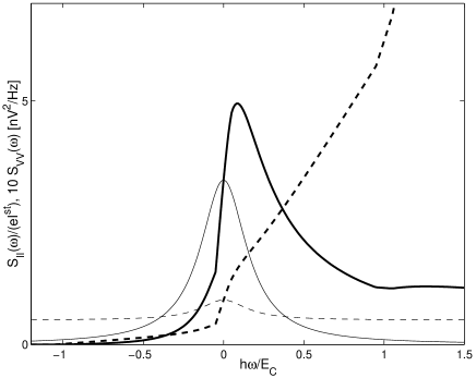
Figure 5.  : Calculated $S_{VV}(\omega)$ (bold solid line) and $S_{II}(\omega)$ (bold dashed line) for a symmetric SET at zero temperature with $R_{T}^{L}=R_{T}^{R}=R_{K}$ and $E_{C}=3\,k_{B}$. The thin lines are the results from orthodox theory. The SET is biased at $n_{x}=0.25$, and slightly above the Coulomb threshold $eV=1.1E_{C}$, with $I^{st}\approx 0.5\mathrm{nA}$. Both $S_{VV}(\omega)$ and $S_{II}(\omega)$ go to zero at $\hbar\omega=1.05E_{C}$ which correspond to the maximal extractable energy.

In the limit $\omega\rightarrow 0$ the orthodox results are recovered. The quantum corrections in the low-frequency regime are discussed in detail for the two-level system in section 4.2. The noise at large negative frequencies, which correspond to noise where the SET emits large energies, tend to zero. In our approximation the voltage noise is analytically zero when $P_{n}^{st}\Gamma_{n\pm}(\omega)=0$ for all $n$, i.e. when no inelastic tunneling events are allowed from the steady-state. The shot-noise part of the current noise behaves similarly, and the correction has the same order of magnitude as the cotunneling shot-noise, which we do not take into account. Therefore, to the accuracy of our approximation, the current noise vanishes when the shot-noise vanishes, i.e. when $P_{n}^{st}\Gamma_{n\pm}(\omega)=0$ for all $n$.

In the high positive frequency limit the spectral noise density of the SET should be independent of the bias and be dominated by the Nyquist noise in Eq. (3). In this limit all rates entering the quantum noise formulas simplify to

$$\Gamma_{n\pm}^{L/R}(\omega)\rightarrow\Gamma^{L/R}\equiv\frac{R_{K}}{2R_{T}^{L/R}}\frac{\omega}{2\pi}+O(1)=\frac{\hbar\omega}{2e^{2}R_{T}^{L/R}}+O(1),$$ (19)

where $O(1)$ is a bias-dependent constant. Using $S_{VV}(\omega)=e^{2}/C_{\Sigma}^{2}\ S_{NN}(\omega)$ we thus arrive at the following high-frequency quantum noise expressions

$$S_{VV}(\omega)\approx\frac{2e^{2}}{\omega^{2}C_{\Sigma}^{2}}2(\Gamma^{L}+\Gamma^{R}),\ \ S_{II}(\omega)\approx S_{II}^{shot}(\omega)\approx 4e^{2}(\alpha_{L}^{2}\Gamma^{L}+\alpha_{R}^{2}\Gamma^{R}),$$ (20)

where we used that $\sum_{n}P_{n}^{st}=1$. One may easily check that this agrees with Eq. (3).

4 Two level approximation for the SET

As an explicit example we now show the analytically solvable case with low bias and temperature, such that only the two lowest energy charge states, say $N=0$ and $N=1$, are occupied, i.e. the only non-zero rates are $\Sigma_{0+}$ and $\Sigma_{1-}$.

4.1 Orthodox Theory

The master equation Eq. (4) then simplifies to

$$\partial_{t}\left(\begin{array}[]{c}P_{0}(t)\\ P_{1}(t)\end{array}\right)=\left(\begin{array}[]{cc}-\Sigma_{0+}&\Sigma_{1-}\\ \Sigma_{0+}&-\Sigma_{1-}\end{array}\right)\left(\begin{array}[]{c}P_{0}(t)\\ P_{1}(t)\end{array}\right).$$ (21)

with the solution given by the time-evolution operator

$$\hat{\Pi}(t)=\left(\begin{array}[]{cc}P^{st}_{0}&P^{st}_{0}\\ P^{st}_{1}&P^{st}_{1}\end{array}\right)+\left(\begin{array}[]{cc}P^{st}_{1}&-P^{st}_{0}\\ -P^{st}_{1}&P^{st}_{0}\end{array}\right)e^{-\Sigma t}\ \ (t>0),$$ (22)

where we defined the sum rate $\Sigma=\Sigma_{0+}+\Sigma_{1-}$, and the steady-state occupation probabilities $P^{st}_{0}=\Sigma_{1-}/\Sigma$ and $P^{st}_{1}=\Sigma_{0+}/\Sigma$. The first term in the time evolution matrix (operator) $\Pi(t)$ gives the steady-state solution, and the second term shows simple exponential relaxation with a single rate $\Sigma$ towards the steady state. The charge and tunnel current operators are

$$\hat{N}=\left(\begin{array}[]{cc}0&0\\ 0&1\end{array}\right),\ \hat{I}_{L}=e\Sigma_{0+}\left(\begin{array}[]{cc}0&0\\ 1&0\end{array}\right),\ \hat{I}_{R}=e\Sigma_{1-}\left(\begin{array}[]{cc}0&1\\ 0&0\end{array}\right).$$ (23)

The steady-state properties and correlation functions are

$$N^{st}=P_{1}^{st},\ I^{st}_{L}=I^{st}_{R}=P_{0}^{st}\Sigma_{0+}=P_{1}^{st}\Sigma_{1-},$$

$$K_{NN}(\tau)=P^{st}_{0}P^{st}_{1}e^{-\Sigma\tau},\ \ S_{NN}(\omega)=\frac{2I^{st}}{\omega^{2}+\Sigma^{2}}=\frac{P_{0}^{st}\Sigma_{0+}+P_{1}^{st}\Sigma_{1-}}{\omega^{2}+\Sigma^{2}},$$

$$K_{II}(\tau)=$$

$$=eI^{st}[(\alpha_{R}^{2}+\alpha_{L}^{2})\delta(\tau)+(\alpha_{L}\Sigma_{0+}-\alpha_{R}\Sigma_{1-})(\alpha_{R}\Sigma_{0+}-\alpha_{L}\Sigma_{1-})\frac{e^{-\Sigma\tau}}{\Sigma}],$$

$$S_{II}(\omega)=eI^{st}[(\alpha_{R}^{2}+\alpha_{L}^{2})+2\frac{(\alpha_{L}\Sigma_{0+}-\alpha_{R}\Sigma_{1-})(\alpha_{R}\Sigma_{0+}-\alpha_{L}\Sigma_{1-})}{\Sigma^{2}+\omega^{2}}]=$$

$$=eI^{st}\frac{\Sigma_{0+}^{2}+\Sigma^{2}_{1-}+\omega^{2}(\alpha_{R}^{2}+\alpha_{L}^{2})}{\Sigma^{2}+\omega^{2}}.$$ (24)

Notice that both charge- and current-noise are proportional to the steady-state current.

4.2 Low Frequency Quantum Theory

In the finite but low-frequency regime, i.e. when still only $\Gamma^{L}_{0+}(\omega)$ and $\Gamma^{R}_{1-}(\omega)$ are non-zero, the quantum expressions simplify to:

$$S_{NN}(\omega)=\frac{P_{0}^{st}2\Gamma^{L}_{0+}(\omega)+P_{1}^{st}2\Gamma^{R}_{1-}(\omega)}{\omega^{2}+(\Sigma_{0+}(\omega)+\Sigma_{1-}(\omega))^{2}},$$

$$S_{II}(\omega)=2e^{2}\left[P_{0}^{st}\alpha_{L}^{2}\Gamma^{L}_{0+}+P_{1}^{st}\alpha_{R}^{2}\Gamma^{R}_{1-}\right]+\frac{\alpha_{L}\Sigma_{0+}-\alpha_{R}\Sigma_{1-}}{\omega^{2}+(\Sigma_{0+}+\Sigma_{1-})^{2}}\times$$

$$\times\left[eI^{st}(\Sigma_{0+}-\Sigma_{1-})+2e^{2}(\Sigma_{0+}+\Sigma_{1-})(P_{1}^{st}\alpha_{R}\Gamma^{R}_{1-}-P_{0}^{st}\alpha_{L}\Gamma^{L}_{0+})\right],$$

where the frequency dependence of $\Sigma_{n\pm}(\omega)$ and $\Gamma_{n\pm}^{L/R}(\omega)$ has been suppressed for brevity. At zero temperature, with symmetric junctions $C_{L}=C_{R}$ and $R_{T}^{L}=R_{T}^{R}=R_{T}$, the expressions simplify further:

$$S_{NN}(\omega) = \frac{1}{e}\left[I^{st}+\frac{\hbar\omega}{eR_{T}}\right]\frac{1}{(\Sigma_{0+}(0)+\Sigma_{1-}(0))^{2}+\omega^{2}},$$

$$S_{II}(\omega) = \frac{e}{2}\left[I^{st}+\frac{\hbar\omega}{2eR_{T}}\right]\left[1+\frac{(\Sigma_{0+}(0)-\Sigma_{1-}(0))^{2}}{(\Sigma_{0+}(0)+\Sigma_{1-}(0))^{2}+\omega^{2}}\right].$$ (26)

We find that the classically derived expressions (Eq. 4.1), symmetric in $\pm\omega$, get an asymmetric quantum correction linear in $\omega$. The correction is added to the steady-state current and is proportional to $\hbar\omega/eR_{T}$, which would be the current through one junction with voltage bias $V=\hbar\omega/e$.

Thus the important difference between the orthodox result and the full quantum result is that we get an asymmetry in the noise spectrum between the positive and negative frequencies in the full quantum result. This becomes important for example in a qubit measurement since it will drastically change the occupation of the two levels in the qubit. In the next sections we will discuss such a qubit, and how the noise from the SET will affect the measurement of the qubit.

5 The Qubit

The qubit we consider is made up of the two lowest lying energy levels in a single Cooper-pair box (SCB) [17]. An SCB is a small superconducting island, with charging energy $E_{C}^{qb}=e^{2}/2(C_{qb}+C_{g}^{qb}+C_{c})$, coupled to a superconducting reservoir via a Josephson junction with Josephson energy $E_{J}$. In order to have a good qubit the following inequalities have to be fulfilled: $\Delta_{s}>E_{C}^{qb}\gg E_{J}\gg k_{B}T$, where $\Delta_{s}$ is the superconducting energy gap and $T$ is the temperature. The low temperature is required to prevent thermal excitations and the high superconducting gap is needed to suppress quasiparticle tunneling. For suitable values of the gate voltage (close to $n_{g}=1/2$) the box can be described by the following two-level Hamiltonian [17, 15]

$$H^{qb}_{q}=-\frac{4E_{C}^{qb}}{2}(1-2n_{g})\hat{\sigma}_{z}-\frac{E_{J}}{2}\hat{\sigma}_{x}$$ (27)

written in the charge basis ${\left\langle{\uparrow}\right|}={\left\langle{n=0}\right|}\equiv(1\ 0),{\left\langle{\downarrow}\right|}={\left\langle{n=1}\right|}\equiv(0\ 1)$, where $n$ is the number of extra Cooper-pairs on the island, $\hat{\sigma}_{x,z}$ are the Pauli matrices, and $n_{g}=C_{g}V_{g}/2e$ is the number of gate-induced Cooper-pairs. By changing the gate voltage the eigenstates of the qubit can be tuned from being almost pure charge states to a superposition of charge states. The eigenstates of the system written in the charge basis are

$${\left|{0}\right\rangle} = \cos(\eta/2){\left|{\uparrow}\right\rangle}+\sin(\eta/2){\left|{\downarrow}\right\rangle}$$

$${\left|{1}\right\rangle} = -\sin(\eta/2){\left|{\uparrow}\right\rangle}+\cos(\eta/2){\left|{\downarrow}\right\rangle},$$ (28)

where $\eta=\arctan(E_{J}/4E_{qb}(1-2n_{g}))$ is the mixing angle. The energy difference between the two states is $\Delta E=\sqrt{(4E_{qb})^{2}(1-2n_{q})^{2}+E_{J}^{2}}$ and the average charge of the eigenstates is

$$Q_{0}=2e\langle 0|\downarrow\rangle\langle\downarrow|0\rangle=2e\sin^{2}(\eta/2),\ \ Q_{1}=2e\langle 1|\downarrow\rangle\langle\downarrow|1\rangle=2e\cos^{2}(\eta/2).$$ (29)

6 SET Charge Measurement of Qubit

We assume that the qubit is in the state $c_{0}(0){\left|{0}\right\rangle}+c_{1}(0){\left|{1}\right\rangle}$ before a measurement. A perfect charge measurment, i.e. qubit read-out, will now give the charge $Q_{0}$ or $Q_{1}$ with probability $|c_{0}|^{2}$ and $|c_{1}|^{2}$ respectively. The two qubit states correspond to slightly different SET gate voltages, and therefore to two slightly different sets of transition rates, and two different steady-state currents $I^{st}_{0}$ and $I^{st}_{1}$. The current fluctuates so there is a finite measurement time $t_{m}$ needed to separate $I^{st}_{0}$ from $I^{st}_{1}$[15]

$$t_{m}^{theory}=\frac{(I^{st}_{1}-I^{st}_{0})^{2}}{8S_{II}(0)}\approx\frac{e^{2}R_{T}C_{\Sigma}}{\Delta Q^{2}}.$$ (30)

where $\Delta Q=(Q_{1}-Q_{0})\cdot C_{c}/C_{qb}$ is the charge difference seen by the SET, and where for the last estimate have we used a symmetric SET biased slightly above the Coulomb threshold at $n_{x}=0.25$. The experimentally determined charge sensitivity $\delta Q$ gives the measurement time according to

$$t_{m}^{exp}=\left(\frac{2\delta Q}{\Delta Q}\right)^{2},$$ (31)

and by comparing Eq. (30) and Eq. (31) we may deduce a rough theoretical estimate for the charge sensitivity $\delta Q^{theory}$. For the parameters of sample # 1 and # 2 listed in Table 1 we find $\delta Q^{theory}=e\sqrt{R_{T}C_{\Sigma}}/2\sim 1.5\cdot 10^{-6}e/\sqrt{Hz}$, which further substantiates that the measurements are indeed almost shot noise limited.

7 SET Back Action on the Qubit

When performing a measurement on a qubit, the measurement necessarily dephases the qubit. However, there can also be transitions between the two qubit states which destroys the information that the read-out system tries to measure. This mixing occurs due to charge fluctuations of the SET island $S_{NN}(\omega)$, which creates a fluctuating charge on the coupling capacitance $C_{c}$, which is equivalent to a fluctuating qubit gate charge $n_{g}\rightarrow n_{g}+\delta n_{g}(t)$. The characteristic time for this mixing process is the time $t_{mix}$. In the weak coupling limit $C_{c}\ll\{C_{\Sigma},C_{qb}\}$, which is relevant for the qubit measurement setup, we may use pertubation theory to evaluate $t_{mix}$.

The fluctuating term in the qubit Hamiltonian, written in the charge basis is

$$\delta H^{qb}_{q}(t)=\frac{4E_{qb}}{2}2\delta n_{g}(t)\hat{\sigma}_{z}=E_{I}\delta n(t)\hat{\sigma}_{z},\ \ E_{I}=\frac{2e^{2}C_{c}}{C_{qb}C_{\Sigma}},$$ (32)

where $e\ \delta n(t)$ represents the fluctuations of charge on the SET-island, and where we have omitted the term quadratic in $\delta n_{g}(t)$. We also defined an electrostatic SET-qubit interaction energy $E_{I}$. In the eigenbasis, the full qubit Hamiltonian now reads

$$\delta H_{e}(t)=-\frac{\Delta E}{2}\hat{\sigma}_{z}+E_{I}\delta n(t)(\cos(\eta)\hat{\sigma}_{z}+\sin(\eta)\hat{\sigma}_{x}).$$ (33)

The $\cos(\eta)$ term leads to dephasing, and the $\sin(\eta)$ term to interlevel transitions (level mixing and relaxation).

Weak coupling means $E_{I}\ll\{E_{C},E_{C}^{qb}\}$ and we may use standard second order time-dependent pertubation theory[30] to see the effect of the charge fluctuations. Assuming that the qubit is in a pure coherent state $c_{0}(0){\left|{0}\right\rangle}+c_{1}(0){\left|{1}\right\rangle}$ at time $t=0$, we may express the effect of the fluctuating SET charge in terms of the time-evolution of the quantities $P^{qb}_{0}(t)=|c_{0}(t)|^{2},P^{qb}_{1}(t)=|c_{1}(t)|^{2}$ and $\xi(t)=|c_{0}(t)c_{1}^{*}(t)|$. In terms of the qubit density-matrix, $P^{qb}_{0,1}(t)$ are the diagonal elements, determining the occupation of respective state, and $\xi(t)$ is the magnitude of the off-diagonal elements, describing the quantum coherence between the states. We find that the qubit occupation probabilities obey a similar master equation as the two-level SET (Eq. (21)), where now the transisition rates are determined by the spectral density of the charge fluctuations at the frequency corresponding to the qubit level splitting:

$$\Sigma^{qb}_{0+}=\frac{E^{2}_{I}\sin^{2}\eta}{\hbar^{2}}S_{NN}(\Delta E/\hbar),\ \ \Sigma^{qb}_{1-}=\frac{E^{2}_{I}\sin^{2}\eta}{\hbar^{2}}S_{NN}(-\Delta E/\hbar),$$ (34)

where $S_{NN}(\omega)$ is the asymmetric charge (number) noise spectral density defined in Eq. (10). The qubit therefore relaxes exponentially on the timescale $t_{mix}$, where

$$t_{mix}^{-1}=\Sigma_{qb}=\Sigma^{qb}_{0+}+\Sigma^{qb}_{1-},$$ (35)

towards the steady-state $P_{0}^{qb,st}=\Sigma^{qb}_{1-}/\Sigma^{qb}$, $P_{1}^{qb,st}=\Sigma^{qb}_{0+}/\Sigma^{qb}$. One may note that the quantum corrections in Eq. (4.2) cancel in the expression $S_{NN}(\omega)+S_{NN}(-\omega)$ determining the mixing time.

Due to the charge fluctuations the quantum coherence decays exponentially

$$\xi(t)=\xi(0)e^{-t/\tau_{\varphi}},\ \ \tau^{-1}_{\varphi}=2\frac{E^{2}_{I}\cos^{2}\eta}{\hbar^{2}}S_{NN}(0)+\frac{\Sigma^{qb}}{2},$$ (36)

where $\tau_{\varphi}$ is the timescale for dephasing.

7.1 Signal to Noise Ratio in Qubit Read Out

Now we can use the measured data for samples #1 and #2 to calculate both $t_{m}$ and $t_{mix}$, and thus we can also get the expected signal-to-noise ratio for a single-shot measurement, which is simply given by $SNR_{SS}=\sqrt{t_{mix}/t_{m}}$. The spectral densities $S_{VV}(f)$ for the two samples at the optimum charge sensitivity, at a current of 6.7 and 8.0 nA for samples #1 and #2, respectively, are displayed in Fig. 6. As can be seen both through Eq. (34) and in Fig. 6, the mixing time increases strongly with increasing $\Delta E$. In our case $\Delta E$ is limited by the superconducting energy gap $\Delta$, which for aluminum films corresponds to about 2.5 K. Using niobium as the qubit material would substantially increase the mixing time. If we assume that $E^{qb}_{C}$ and thus also $\Delta E$ can be scaled with $\Delta$ and that the coupling $C_{c}/C_{qb}$ is kept constant, mixing times of several ms can be reached. In that case, other sources than the SET noise would most probably dominate the mixing. The results for the samples #1 and #2 are summarized in Table 1, where a coupling $C_{c}/C_{qb}=0.01$ is assumed.

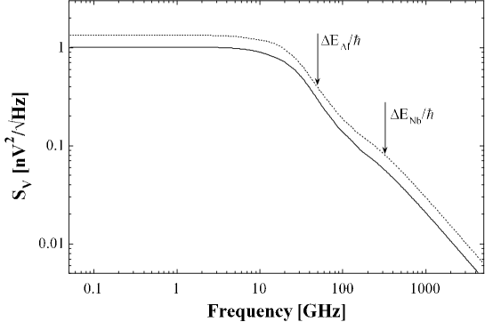
Figure 6.  : Calculated $S^{sym}_{VV}(f)$ for samples #1(full line) and #2(dashed line). The arrows show the energy separations of the two qubit states for an aluminum and a niobium qubit, respectively.

TABLE 1.  :

 SET Qubit $\delta Q$ $\Delta E$ $S_{V}(\omega)$ $t_{m}$ $t_{mix}$ SNR Sample material e/$\sqrt{\rm{Hz}}$ [K] [nV²/Hz] [$\mu$s] [$\mu$s]  1 Al 6.3 2.4 0.29 0.40 8.6 4.6 1 Nb 6.3 15.5 0.056 0.40 1860 68 2 Al 3.2 2.4 0.39 0.10 6.4 8.0 2 Nb 3.2 15.5 0.080 0.10 1300 114  

7.2 Coulomb Staircase

One may use the SET to measure the so-called Coulomb staircase, i.e. the average charge of the qubit as a function of gate voltage. In an ideal situation with no energy availible from an external source, at zero temperature, the qubit would follow the ground state adiabatically and the charge would increment in steps of $2e$ at $n_{g}=n+0.5$, $n$ integer. These steps are not perfectly sharp because of the Josephson energy mixing the charge states[17]. Now assuming that the qubit equilibrium is determined by the SET back action the charge measured should instead be $P_{0}^{qb,st}Q_{0}+P_{1}^{qb,st}Q_{1}$. The steps are now rounded further[32] due to the finite probability for the qubit to be excited, see Fig. 7. The quantum asymmetry of the noise-spectrum, indicating the difference of qubit excitation and relaxation, is vital to recover the correct Coulomb staircase. Straighforward use of orthodox theory would predict an equal population of the qubit states.

Figure 7.  : The calculated Coulomb staircase of an SCB as measured by the SET, assuming that the SET backaction determine the steady-state of the qubit.

References

• [1] T. A. Fulton and G. J. Dolan, Phys. Rev. Lett. 59, 109 (1987)
• [2] K. K.Likharev, IEEE Trans. Mag. 23, 1142 (1987)
• [3] D. V. Averin and K. K. Likharev: in Mesoscopic Phenomena in Solids, eds. B.L. Altshuler, P.A. Lee and R.A. Webb (North-Holland, Amsterdam, 1991) p. 173.
• [4] H. Grabert and M. H. Devoret, NATO Adv. Study Inst. Ser., Ser. B 279, 74 (1992).
• [5] K. Matsumoto, M. Ishii, K. Segawa, Y. Oka, B. J. Vartanian and J. S. Harris, Appl. Phys. Lett. 68, 35 (1996)
• [6] Yu. A. Pashkin, Y. Nakamura, and J. S. Tsai Appl. Phys. Lett. 76, 2256 (2000)
• [7] T. W. Kim, D. C. Choo, J. H. Shim, and S. O. Kang Appl. Phys. Lett., 80, 2168 (2002)
• [8] R. J.Schoelkopf, P. Wahlgren, A. A. Kozhevnikov, P. Delsing, and D. E. Prober, Science 280, 1238 (1998)
• [9] J. Pettersson, P. Wahlgren, P. Delsing, D. B. Haviland, T. Claeson, N. Rorsman and H. Zirath, Phys.l Rev. B 53, R13272, (1996)
• [10] S. L Pohlen, R. J. Fitzgerald, J. M. Hergenrother, and M. Tinkham, Appl. Phys. Lett. 74, 2884-2886 (1999)
• [11] A. Aassime, D.Gunnarsson, K. Bladh, P. Delsing, and R. Schoelkopf, Appl. Phys. Lett. 79, 4031 (2001)
• [12] A. Aassime, G. Johansson, G. Wendin, P. Delsing, and R. Schoelkopf, Phys. Rev. Lett. 86, 3376 (2001)
• [13] M. J. Lea, P. G. Frayne, and Yu. Mukharsky, Fortschr. Phys. 48, 1109 (2000)
• [14] B. E. Kane, N. S. McAlpine, A. S. Dzurak, R. G. Clark, G. J. Milburn, He. Bi. Sun and Howard Wiseman, Phys. Rev. B, 61, 2961 (2000)
• [15] Y. Makhlin, G. SchΓΆn, and A. Shnirman Rev. Mod. Phys., 73, 357 (2001)
• [16] T. R. Stevenson,A. Aassime, P. Delsing, R. Schoelkopf, K. Segall, and C. M. Stahle, IEEE Transactions On Applied Superconductivity 11, 692 (2001)
• [17] V. Bouchiat, D. Vion, P. Joyez, D. Esteve and M. H. Devoret, Phys. Scripta T76, 165 (1998)
• [18] G L Ingold, Yu V Nazarov in: NATO ASI Series B: Physics, vol. 294, Single Charge Tunneling: Coulomb Blockade Phenomena in Nanostructures, Eds. H Grabert, M Devoret, p. 21-106
• [19] L. J. Geerligs, D. V. Averin, and J. E. Mooij Phys. Rev. Lett. 65, 3037 (1990)
• [20] W. Shockley, Journal of Applied Physics, 9, 635 (1938)
• [21] Ya. M. Blanter and M. Buttiker, Phys. Rep. 336, 1 (2000)
• [22] A. N. Korotkov, Phys. Rev. B, 59, 10 381 (1994)
• [23] L. Fedichkin and V. V’yurkov, Appl. Phys. Lett., 64 2535 (1994)
• [24] U. Hanke, Yu. M. Galperin, and K. A. Chao, Physical Review B 50, 1595 (1994)
• [25] G. R. Grimmett, and D. R. Stirzaker, Probability and Random Processes, (Clarendon Press, Oxford, 1992), 245
• [26] H. B. Callen and T. A. Welton, Phys. Rev., 83, 34 (1951)
• [27] G. Johansson, A. KΓ€ck and G. Wendin, Phys. Rev. Lett. 88, 046802 (2002)
• [28] W. Schottky, Annals of Physics (Leipzig) 57 541 (1918)
• [29] H. Schoeller and G. SchΓΆn, Phys. Rev. B, 50, 18 436 (1994).
• [30] J. J. Sakurai, Modern Quantum Mechanics, (Addison-Wesley, 1985)
• [31] F. Dyson, Phys. Rev. 75, 1736 (1949)
• [32] Y. V. Nazarov, J. Low Temp. Phys. 90 77 (1993)