Onset of incommensurability in quantum spin chains

Abstract

In quantum spin chains, it has been observed that the incommensurability occurs near valence-bond-solid (VBS)-type solvable points, and the correlation length becomes shortest at VBS-type points. Besides, the correlation function decays purely exponentially at VBS-type points, in contrast with the two-dimensional (2D) Ornstein-Zernicke type behavior in other regions with an excitation gap. We propose a mechanism to explain the onset of the incommensurability and the shortest correlation length at VBS-like points. This theory can be applicable for more general cases.

Frustration is one of the important problem in many-body physics. Recently, many things in frustrated systems become clearer with field theoretical approaches and numerical calculations (density matrix renormalization group (DMRG) etc.). However, relatively little is known about commensurate-incommensurate (C-IC) transitions induced by frustration in quantum spin systems. Among them, it is observed the C-IC change in the region with an excitation gap (therefore, it is not a phase transition) in one-dimensional (1D) quantum spin models.

For example, the C-IC change begins from the Majumdar-Ghosh point [1] in the S=1/2 next-nearest-neighbor (NNN) chain

$$H=\sum_{j}(S_{j}S_{j+1}+\alpha S_{j}S_{j+2}),$$ (1)

($\alpha_{D}=1/2$ is the solvable point), or from the valence-bond-solid (VBS) point [2] in the S=1 bilinear-biquadratic chain,

$$H=\sum_{j}(S_{j}S_{j+1}+\alpha(S_{j}S_{j+1})^{2}),$$ (2)

($\alpha_{D}=1/3$ is the solvable point).

With a numerical diagonalization, Tonegawa and Harada observed in the S=1/2 NNN chain [3] that the incommensurability of the spin correlation begins near the solvable point. However, from the DMRG calculation, Bursill et al. stated that in the static structure factor (Fourier transform of spin-correlation function), the C-IC change begins slightly different from the solvable point for the S=1 bilinear-biquadratic chain [4], and for the S=1/2 NNN chain [5]. In contrast, using the DMRG, Schollwöck, Jolicoeur, and Garel [6] have closely investigated the correlation function of the S=1 bilinear-biquadratic chain (2), not the structure factor, and they found that the incommensurability begins right at the VBS point. Adding this, they have pointed out the singular behavior of the modulation wavenumber.

Secondly, it has been noticed that the correlation length is shortest at the VBS-type point.

Thirdly, at the VBS-type point, the spin-correlation function decays purely exponentially, in contrast with the 2D (1+1D) Ornstein-Zernicke type (that is, 2D Green function for the free massive particle) behavior in the other region with a gap.

Although Schollwöck et al. have tried to explain these features on the analogy of the 1D classical frustrated Ising spin with finite temperature, several features are different from the quantum spin chain case, which we intend to explain in this study. After that, Kolezhuk, Roth, and Schollwöck applied their idea to the S=1 NNN chain [7, 8], where they called the shortest correlation length point as the “disordered point”, generalizing the VBS-type point with the above features.

Recently, Fáth and Sütõ proposed an effective field theory [9] to explain these features in the C-IC change of the S=1 bilinear-biquadratic chain. Although their results seem natural, they have not derived their effective field theory directly from the lattice Hamiltonian. And from their theory, the C-IC change near the Majumdar-Gosh point cannot be explained. Therefore, it is meaningful to construct a theory on firmer ground. Considering the analyticity of the structure factor $S(q)$ around the disordered point, where several exact results are known, we propose another approach to this problem. Since, what we observe experimentally is not Hamiltonian itself, but structure factors or other quantities, thus our approach may be more natural in a physical sense.

We summarize the results by Schollwöck et al. as (see also Fig.1)

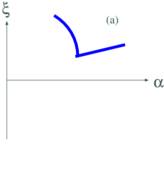
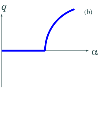
Figure 1: Singular behaviors of correlation length (a) and wave number (b).

1. In the commensurate region ($\alpha<\alpha_{D}$), the correlation function behaves as the 2D Ornstein-Zernicke-type

   $$\langle S_{0}S_{n}\rangle\approx(-1)^{n}|n|^{-1/2}\exp(-|n|/\xi(\alpha)),$$ (3)

   where far enough from the disordered point $\alpha_{D}$.

2. In the incommensurate region ($\alpha>\alpha_{D}$) ,

   $$\langle S_{0}S_{n}\rangle\approx(-1)^{n}\cos(q(\alpha)n)|n|^{-1/2}\exp(-|n|/\xi(\alpha)),$$ (4)

   where far enough from the disordered point $\alpha_{D}$.

3. At the disordered point $\alpha_{D}$,

   $$\langle S_{0}S_{n}\rangle\approx(-1)^{n}\exp(-|n|/\xi(\alpha_{D})).$$ (5)

4. From the commensurate side,

   $$\frac{d\xi(\alpha)}{d\alpha}|_{\alpha_{D}}=-\infty.$$ (6)

5. From the incommensurate side,

   $$\frac{dq(\alpha)}{d\alpha}|_{\alpha_{D}}=\infty.$$ (7)

6. From the incommensurate side, by fitting as

   $$q(\alpha)\propto(\alpha-\alpha_{D})^{\sigma},$$ (8)

   we obtain $\sigma\approx 1/2$.

7. Neither the $\exp(-|n|/\xi)$ nor the $|n|^{-1/2}\exp(-|n|/\xi)$ form cannot describe the correlation function near the disordered point $\alpha_{D}$.

Note that, strictly speaking, the 2D Ornstein-Zernicke form is the modified Bessel function [10],

$$G(\vec{n})=\int\frac{\exp(i\vec{q}\cdot\vec{n})d^{2}q}{\vec{q}^{2}+\xi^{-2}}=2\pi K_{0}(|n|/\xi),$$ (9)

which behaves $|n|^{-1/2}\exp(-|n|/\xi)$ in large distance. And static correlation function is

$$G(0,n_{1})=\pi\int\frac{\exp(iq_{1}n_{1})}{\sqrt{q_{1}^{2}+\xi^{-2}}}dq_{1}.$$ (10)

To explain these features, we consider the static structure factor in the complex $q$ plain,

$$S(q)\equiv\sum_{n}\exp(iqn)(-1)^{n}\langle S_{0}S_{n}\rangle.$$ (11)

The simple minded Fourier transforms of the correlation functions are

1. At the disordered point,

   $$S(q)\propto\frac{1}{q^{2}+m^{2}}.$$ (12)

2. In the commensurate region,

   $$S(q)\propto\frac{1}{\sqrt{q^{2}+m^{2}}}.$$ (13)

3. In the incommensurate region,

   $$S(q)\propto\frac{1}{\sqrt{(q-q(\alpha))^{2}+m^{2}}}+\frac{1}{\sqrt{(q+q(\alpha))^{2}+m^{2}}}.$$ (14)

However, with the above forms, one cannot connect these three region. In fact, in terms of the singularity in the complex $q$ plain, there are poles at the disordered point, in contrast with the branch-cuts in the other (commensurate, incommensurate) regions.

In order to unify these three region, we reconsider the relation between the pole and the branch-cut. A pole and a branch-cut can be deformed each other as following,

$$f(z)\equiv(z^{2}-d)^{-1/2},$$ (15)

which has two branch-points at $z=\pm\sqrt{d}$ for $d>0$, a pole at $z=0$ for $d=0$, and two branch-points at $z=\pm i\sqrt{|d|}$ for $d<0$. Note that $f(z)$ is an odd function $f(-z)=-f(z)$, considering the analytic continuation around the branch-cut.

Besides, to relate it with physical phenomena, we consider the following assumptions:

1. $S(q)$ is analytic except several algebraic singular points.

2. $S(q)$ is real on the real axis $(S(q)=\bar{S}(\bar{q}))$.

3. From parity, $S(q)=S(-q)$.

4. $S(q)$ is varied continuously with a parameter $\alpha$.

5. At the disordered point $\alpha_{D}$, $S(q)$ is described with two poles.

6. Singular points and branch-cuts should not cross the real axis.

From these assumptions, we can obtain the simplest singularity structure as Fig. 2, that is, there are two poles symmetric with real axis, or four branch-points continuously deformable from them. The static structure factor, originated from the singular terms, is given as

$$S_{sing}(q) = Af(q+\tilde{m}i)f(q-\tilde{m}i)$$ (16)

$$= A[q^{4}+2(\tilde{m}^{2}-d)q^{2}+\tilde{m}^{4}+d^{2}+2\tilde{m}^{2}d]^{-1/2},$$

where real parameters $A,\tilde{m},d$ may depend on $\alpha$, especially $d\propto\alpha-\alpha_{D}$. Although this result for the static structure is the same as in [9], our theory is based on the analyticity of $S(q)$ and the exact $S(q)$ at the VBS point. Note that without the assumption for algebraic singularities, there remain other possibilities

$$S_{sing}(q) = A\frac{i}{2\tilde{m}}[f(q+\tilde{m}i)-f(q-\tilde{m}i)]$$ (17)

$$= \frac{A}{\tilde{m}}\frac{1}{\sqrt{(q^{2}-\tilde{m}^{2}-d)^{2}+4q^{2}\tilde{m}^{2}}}\cos\left(\frac{1}{2}\arctan(\frac{2q\tilde{m}}{q^{2}-\tilde{m}^{2}-d})\right),$$

$$S_{sing}(q) = A\frac{1}{2q}[f(q+\tilde{m}i)+f(q-\tilde{m}i)].$$ (18)

The assumption for algebraic singularities physically relates to the locality of interactions[11].

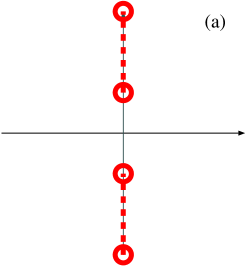
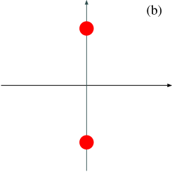
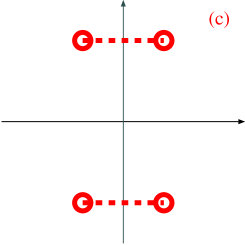
Figure 2: Continuous deformation of branch-cuts and poles. They correspond to commensurate region (a), disordered point (b), incommensurate region (c),

Although it seems reasonable four branch-points in the incommensurate region, how do we interpret four branch-points in the commensurate region? In the large distance, or the small wave number $q$, to $S(q)$ on the real axis mainly contribute the two branch-points closer to the real axis, thus it seems only two branch-points when $0<1-|d|/\tilde{m}^{2}\ll 1$ .

When we set $d\approx c_{1}(\alpha-\alpha_{D});\;c_{1}>0$ in eq. (16), we can explain systematically the singular behaviors of $\xi(\alpha),q(\alpha)$ near the disordered point $\alpha_{D}$. And we can calculate the analytic form for $S(q)$ in the neighborhood of $\alpha_{D}$. In addition, near $\alpha_{D}$, $\tilde{m}$ may behave as $\tilde{m}\approx\tilde{m}_{0}+c_{2}(\alpha-\alpha_{D})$. It should be $c_{2}<0$, since the correlation length increases in the incommensurate region.

Generally, the requirement for the amplitude is $A\neq 0$, since for $A=0$ the correlation function becomes perfectly zero. However, at the Majumdar-Ghosh point in the S=1/2 NNN chain, the correlation function behaves as

$$\langle S_{0}S_{n}\rangle=0,\;(for|n|\geq 2),$$ (19)

which can be interpreted as the $A(\alpha)\propto(\alpha-\alpha_{D})$ case or the $A(\alpha)\propto(\alpha-\alpha_{D})^{2}$ case. The latter possibility comes from that spin variables may depend as $S_{n}\propto(\alpha-\alpha_{D})$.

Until now, we have neglected the lattice structure and the terms which are regular in the whole complex $q$ plain. To include the lattice structure, we should require $S(q)=S(q+2\pi)$. Thus, the full static structure factor is

$$S(q)=\sum_{j=-\infty}^{\infty}S_{sing}(q+2\pi j)+S_{reg}(q),$$ (20)

where

$$S_{reg}(q)\equiv\sum_{j=-\infty}^{\infty}a_{j}\cos(jq).$$

Note that to calculate the spin-correlation function, it is enough to consider the singularities of $S(q)$ within the Brillioun zone, because of periodicity.

In summary, the C-IC change can be regarded as a fusion-fission of singularities in the complex $q$ plain. The Lifshitz point, where the static structure factor changes from a single peak to double peaks, is a natural consequence of this fusion-fission of singularities [6, 7, 8] (see in (16),

$$\frac{\partial^{2}S_{sing}(q)}{\partial q^{2}}(q=0)\propto A(\tilde{m}^{2}-d)$$ (21)

).

The argument in this paper should be checked in the DMRG calculation near the disordered point. After checking the expectation for the static structure factor, one can extend it to the dynamical structure factor. Since the VBS-type states [2] are obtained not only in the 1D quantum system, but also in the 2D and 3D quantum systems, it is interesting whether such C-IC changes may occur at the VBS-type points in higher dimensions.

References

- [1] C. K. Majumdar and D. K. Ghosh: J. Math. Phys. 10 (1969) 1388.
- [2] I. Affleck, T. Kennedy, E. H. Lieb, and H. Tasaki: Phys. Rev. Lett. 59 (1987) 799; Comm. Math. Phys. 115 (1988) 477.
- [3] T. Tonegawa and I. Harada: J. Phys. Soc. Jpn. 56 (1987) 2153.
- [4] R. J. Bursill, T. Xiang, and G. Gehring: J. Phys. A, 28 (1995) 2109.
- [5] R. Bursill, G.A. Gehring, D. J. Farnell, J. B. Parkinson, T. Xiang, and C. Zeng: J. Phys. Condens. Matter.,7 (1995) 8605.
- [6] U. Schollwöck, Th. Jolicoeur, and T. Garel: Phys. Rev. B, 53 (1996) 3304.
- [7] A. Kolezhuk, R. Roth, and U. Schollwöck: Phys. Rev. Lett., 77 (1996) 5142.
- [8] A. Kolezhuk, R. Roth, and U. Schollwöck: Phys. Rev. B, 55 (1997) 8928.
- [9] G. Fáth and A. Sütõ: Phys. Rev. B 62 (2000) 3778.
- [10] Numerically, it is observed that the modified Bessel function shows better fitting than the form in K. Nomura: Phys. Rev. B, 40 (1989) 2421.
- [11] When the lattice Hamiltonian has long-range interactions, the assumption that a finite number of branches and at most algebraic singularities may be broken.