Managing catastrophic changes in a collective

Abstract

We address the important practical issue of understanding, predicting and eventually controlling catastrophic endogenous changes in a collective. Such large internal changes arise as macroscopic manifestations of the microscopic dynamics, and their presence can be regarded as one of the defining features of an evolving complex system. We consider the specific case of a multi-agent system related to the El Farol bar model, and show explicitly how the information concerning such large macroscopic changes becomes encoded in the microscopic dynamics. Our findings suggest that these large endogenous changes can be avoided either by pre-design of the collective machinery itself, or in the post-design stage via continual monitoring and occasional ‘vaccinations’.

A contribution to the Workshop on Collectives and the Design of Complex Systems, organized by David Wolpert and Kagan Tumer, at NASA Ames Research Center, CA, August (2002).

1 Introduction

Understanding the relationship between the overall macroscopic performance of a collective, and its design at the microscopic level, is a high priority for the collectives field (see, for example, Ref. [29]). Typically such performance can be measured in terms of a macroscopic variable of the system which fluctuates in time: for example the level of wastage of a global resource. An example which can be seen in other Chapters of this book, is the discussion of the fluctuations in attendance in the El Farol bar game and related multi-agent models such as the Minority Game. In those cases, one is particularly interested in understanding how to minimize the typical size of such fluctuations and hence ‘optimize’ performance by minimizing the average wastage. In practice, however, typical optimization schemes which focus on minimizing the variance of some global quantity may not be the most relevant. Biology is a wonderful example of a non-optimal system, yet one which does a fantastic job of avoiding catastrophic large changes. The human body, for example, has a complex network of feedback loops set in place in order to ‘survive’. While very few of us exist at our peak level, and even fewer of us hold world records in athletics, we do a pretty good job of coping with everything our changing bodies and changing environment can throw at us. Moreover, the human system can self-manage this difficult situation for up to 100 years, an unimaginable feat for any computer-based system. In short, we may not be optimal in the sense of minimizing wastage, yet our system can handle sudden changes in the environment (i.e. exogenous changes) and also typically manages to resist the tendency to self-generate large unexpected (endogenous) changes or ‘system crashes’.

Large unexpected changes, or so-called extreme events, happen infrequently, yet tend to dictate the long-term dynamical behaviour of real-world systems in disciplines as diverse as biology and economics, through to ecology and evolution. Their consequences are often catastrophic – for example, the sudden jamming of traffic in an information system or on a highway; a fatal change within the human immune system; so-called punctuated equilibria in evolution leading to the sudden extinction of entire species; and crashes in a financial market [2, 18, 24]. The ability to generate large internal, endogenous changes is a defining characteristic of complex systems, and arguably of Nature and Life itself since it leads to evolution through innovation. Thinking through to the management of real-world complex systems and collectives, and in particular the risk associated with such catastrophic changes, one wonders whether these large events could eventually be controlled, or even avoided altogether?

Here we take the first few steps in the direction of ‘risk-management’ in collectives. We consider the specific problem of a complex adaptive multi-agent population, competing for some limited resource. The system is a variant of Arthur’s famous El Farol bar model [1], and exhibits large, self-generated changes. We show that information about the large endogenous changes becomes encoded in the system ahead of the large change itself. The implication is that with a reasonable amount of information, the large change would cease to be a ‘surprise’. The present work therefore has relevance to both the forward and reverse problem in collectives. In ‘pre-design’ collectives – i.e. collectives in which the individual components can be tailor-made to have certain fixed properties – such knowledge could help in the design of ‘safe’ agents whose collective behavior is such that large changes are avoided altogether. In ‘post-design’ collectives – i.e. collectives for which a designer has no control over the properties of the individual components – one could nevertheless hope to control such large changes in order to minimize the potential damage. In particular, one could imagine some form of soft monitoring, whereby an external regulator monitored the system output, detected certain precursors suggesting a dangerous build-up to a large change, then intervened to divert it. Going further, we have recently shown [12] that such systems can actually be ‘vaccinated’ ahead of such large changes thereby affording the system a degree of temporary immunity.

The science of complex systems, as befits its name, lacks a simple definition [25, 30]. It has been used to refer to systems that are intermediate between perfect order and perfect disorder; or even as a simple restatement of the cliché that the behaviour of some systems as a whole can be more than the sum of their parts. Formal definitions of complexity do exist in the computational and information sciences, but apply to specific systems [3]. Here we focus on systems where both the properties of the individual components and the nature of their interactions are reasonably well understood. The constituents themselves can be rather simple, and the relation between any two may also be well understood, yet the collective behavior of the ensemble still manages to escape any simple explanation. A simple example which captures the idea of (co-)evolution and bounded rationality is Arthur’s El Farol bar problem [1]. At its most basic level, this is an example of a game involving a fixed population of players (agents) $N_{tot}$ competing for a limited resource $L$. No more than $L<N_{tot}$ agents can win at each timestep. The agents are adaptive and try to predict the next winning outcome, which is determined only by their own choices. Each agent is equipped with a number of strategies from which to choose, and can do so adaptively based on its present environment. Recent experiments confirm that humans indeed possess such different strategies, despite being faced with the same history [13]. In short, the El Farol bar problem contains the following key ‘complex’ elements:

• A population of heterogeneous agents with bounded rationality.

• Agents who use history-based strategies upon which they base their actions.

• A method of aggregating agent’s behaviour into a global outcome, which introduces feedback into the system.

Our study focuses on a generic multi-agent system, based on the El Farol bar problem, which has already been shown to reproduce statistical and dynamical features similar to those of a real-world complex adaptive system: a financial market. (See www.unifr.ch/econophysics for a detailed account of the extent to which financial markets represent complex systems, and their associated statistical and dynamical properties). Our model also exhibits the crucial feature of seemingly spontaneous large changes of variable duration [20, 21]. Although our study is therefore specific to a particular model, we believe that any multi-agent model which shares the above elements would benefit from the techniques described in this chapter. Recently the concept of an agent has become increasingly important in both artificial intelligence and mainstream computer science [28]. In contrast to the agents considered within El Farol-like complex systems as in this Chapter, the agents in these other fields are typically more sophisticated and are often utilized to perform specific tasks in a wide range of different areas, e.g. e-commerce, classification, information retrieval and management of networks [17, 8]. By studying complex systems involving more basic agents, but which retain the ability to react to their present environment, we aim to develop approaches that may be useful in more complicated collectives comprising richer components.

The Chapter is arranged as follows. In §2 we introduce our generic complex system and in §3 demonstrate its ability to generate time-series which include occasional large movements. In §4 we investigate the game dynamics during these large changes and determine what is occurring microscopically within the model system. In §4.1 we introduce a method of understanding when a large change is possible within the system, and obtain approximate expressions for its duration in §4.2. This leads to an understanding of how such large changes may be avoided.

2 The Grand Canonical Bar Game

We consider a generic complex system in which a population of $N_{tot}$ heterogeneous agents with limited capabilities and information repeatedly compete for a limited global resource. The model is a generalization of Arthur’s bar model where agents will only take part, or play, if they are sufficiently confident of the strategies they hold. A strategy is a forecasting rule that generates a prediction of the next winning outcome based on knowledge of the recent history of winning choices. This is the Grand Canonical Bar Game (GCBG), It captures some of the key behavioural phenomena that are important in collectives/complex systems; those of competition, frustration and adaptability. It is also a ‘minimal’ system of only few parameters.

The GCBG comprises a number of agents $N_{tot}$ who repeatedly decide whether to enter a game where the choices are option A or B. Because of the limited global resource, only agents who are sufficiently confident of winning will participate at each timestep. The outcome at each timestep represents the winning decision, A or B. The agents are adaptive in their strategy choices, but not evolutionary; there is no discovery of new strategies by the agents. A maximum of $L(t)$ agents can win at each timestep. Changing $L(t)$ affects the system’s quasi-equilibrium; hence $L(t)$ can be used to mimic the changing external environment. In the limit that $L(t)$ is time-independent, and all agents are forced to play at each timestep, our model reverts to Arthur’s El Farol bar model. A schematic of the game structure is shown in Figure 1, clearly indicating the feedback present within the system. The method of encoding the outcomes in the game via a binary alphabet, and the associated strategy space, were introduced by Challet and Zhang [5]. However the GCBG differs from the basic Minority Game in its use of an external resource level, and a variable number of participating agents per timestep as a result of the finite confidence level. The agents are of limited yet similar capabilities. Each agent is assigned a ‘brain-size’ $m$; this is the length of the past history bit-string that an agent can use when making its next decision. A common bit-string of the $m$ most recent outcomes is made available to the agents at each timestep. This is the only information they can use to decide which option to choose in subsequent timesteps. Each agent randomly picks $q$ strategies at the beginning of the game, with repetitions allowed. A strategy uses information from the historical record of winning options to generate a prediction [5]. After each turn, the agent assigns one (virtual) point to each of his strategies which would have predicted the correct outcome, and minus one for an incorrect prediction. The resulting time-series appears ‘random’ yet is non-Markovian, with subtle temporal correlations which put it beyond any random-walk based description. Multi-agent games such as the present GCBG may be simulated on a computer, but can also be expressed in analytic form. In the next section we introduce some notation used in the remainder of this chapter.

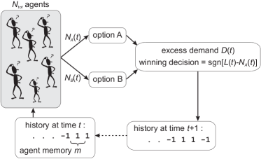
Figure 1: Schematic of game structure.

2.1 Notation

A subset of the agent population, who are sufficiently confident of winning, are active at each timestep. At each timestep $t$ we denote the number of agents choosing option A as $N_{A}(t)$ and the number choosing B as $N_{B}(t)$. If $L(t)-N_{A}(t)>0$ the winning decision is A and vice-versa. The winning decision is thus given by

$$w(t) = \mbox{sgn}\left[L(t)-N_{A}(t)\right],$$

where $\mbox{sgn}[x]$ is the sign function defined by

$$\mbox{sgn}[x]=\begin{cases}-1\quad&\text{for $x<0$},\\ 0&\text{for $x=0$},\\ 1&\text{for $x>0$}.\end{cases}$$

We denote by $w(t)$ the winning option at time $t$, where a value of $1\Rightarrow$ option A, and $-1\Rightarrow$ option B. We frequently have to represent the two possible choices, A or B, in numerical form, and we use the encoding that $1$ always implies option A and $-1$ implies option B. If $w(t)=0$, indicating no clear winning option, this value is replaced with a random coin toss.

The ‘excess demand’ $D(t)=N_{A}(t)-N_{B}(t)$ (which mimics price-change in a market) and number $V(t)=N_{A}(t)+N_{B}(t)$ of active agents (which mimics volume) represent output variables. These two quantities fluctuate with time, and can be combined to construct other global quantities of interest for the complex system studied. We define the cumulative excess demand as $P(t)$. In the context of a financial market, this can be regarded as a pseudo-price. Typically we use the example of a financial market, but the excess demand can be interpreteted in many different circumstances, e.g. as a measure of resource utilization within a system. If we define $L(t)=\phi V(t)$, where $0\leq\phi\leq 1$, then only a fraction $\phi$ of the active population can win. By varying the value of $\phi$, it is possible to change the equilibrium value of $D(t)$, see Figure 2.

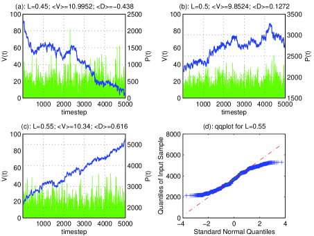
Figure 2: Typical time-evolution of the complex adaptive system for differing values of the global resource level: (a) $L=0.45V(t)$, (b) $L=0.5V(t)$, and (c) $L=0.55V(t)$. In each case, the thick line $P(t)$ represents the cumulative excess demand. For $L$ greater (less) than $0.5N_{tot}$, $P(t)$ has an upward (downward) trend. (d) Corresponding qq-plot for $L=0.55V(t)$ series illustrating the presence of power-law like fat tails. The result for a normal distribution would be a diagonal line, as indicated.

The only global information available to the agents is a common bit-string ‘memory’ of the $m$ most recent outcomes. Consider $m=2$; the $P=2^{m}=4$ possible history bit-strings are $AA$, $AB$, $BA$ and $BB$, with the right-most letter representing the winning choice at the last timestep. The history, or equivalently, the global information available to the agents, can be represented in decimal form $\mu\in\{0,1,\ldots,P-1\}$:

$$\mu(t) = \sum_{i=1}^{m}2^{i-1}\left[w(t-i)+1\right].$$

The global information $\mu(t)$ is updated by dropping the first bit and concatenating the latest outcome to the end of the string.

At the beginning of the game, each agent randomly picks $q$ ($>1$) strategies, making the agents heterogeneous in their strategy sets. This initial strategy assignment is fixed from the outset of each simulation and provides a systematic disorder which is built into each run. This is referred to as the quenched disorder present in the game. An agent decides which option to choose at a given time step based on the prediction of a strategy, which consists of a response, $a^{\mu(t)}\in\{-1,1\}$ to the global information $\mu(t)$. For its current play, an agent chooses its strategy that would have performed best over the history of the game until that time, i.e. has the most virtual points.

Agents have a time horizon $T$ over which virtual points are collected and a threshold probability level $\tau$ which mimics a ‘confidence’. Only strategies having $\geq r$ points are used, where

$$r = T(2\tau-1).$$

We call these active strategies. Agents with no active strategies within their individual set of $q$ strategies do not play at that timestep and become temporarily inactive. Agents with one or more active strategies play the one with the highest virtual point score; any ties between active strategies are resolved using a coin-toss. If an agent’s threshold to play is low, we would expect the agent to play a large proportion of the time as their best strategy will have invariably scored higher than this threshold. Conversely, for high $\tau$, the agent will hardly play at all. The coin-tosses used to resolve ties in decisions (i.e. $N_{A}=N_{B}$) and active-strategy scores, inject stochasticity into the game’s evolution. The implementation of the strategies is discussed in §2.2.

After each turn, agents update the scores of their strategies with the reward function

$$\chi[N_{A}(t),L(t)]=\mbox{sgn}\left[N_{A}(t)-L(t)\right],$$ (1)

namely $+1$ for choosing the correct/winning outcome, and $-1$ for choosing the incorrect outcome. The virtual points for strategy $R$ are updated via

$$S_{R}(t) = \sum_{i=t-T}^{t-1}a_{R}^{\mu(i)}\ \chi\Big{[}N_{A}(i),L(i)\Big{]},$$

where $a_{R}^{\mu(t)}$ is the response of strategy $R$ to global information $\mu(t)$, and the summation is taken over a rolling window of fixed length $T$. To start the simulation, we set the initial strategy scores to be zero: $S_{R}(0)=0$. Because of the feedback in the game, any particular strategy’s success is short-lived. If all the agents begin to use similar strategies, and hence make the same decision, such a strategy ceases to be profitable and is subsequently dropped. This encourages heterogeneity amongst the agent population.

The demand $D(t)$ and volume $V(t)$, which can be identified as the output from the model system, are given by

$$D(t) = \mathbf{n}(t)\cdot\left(\mathbf{a^{\mu(t)}}{\cal H}\Big{[}\mathbf{S}(t)-r\Big{]}\right)\ =\ \sum_{R=1}^{Q}n_{R}(t)a^{\mu(t)}_{R}{\cal H}\Big{[}S_{R}(t)-r\Big{]},$$ (2a)

$$V(t) = \mathbf{n}(t)\cdot{\cal H}\Big{[}\mathbf{S}(t)-r\Big{]}\ =\ \sum_{R=1}^{Q}n_{R}(t){\cal H}\Big{[}S_{R}(t)-r\Big{]}.$$ (2b)

where $n_{R}(t)$ represents the number of agents playing strategy $R$ at timestep $t$.

The demand $D(t)$ is made up of two groups of agents at each timestep: $D_{D}(t)$ agents who act in a deterministic manner, i.e. do not require a coin toss to decide which choice to make - this is because they either have one strategy that is better than their others, or because their highest-scoring strategies are tied but give the same response to the history $\mu(t)$, and $D_{U}(t)$ agents that act in an ‘undecided’ way, i.e. they require the toss of a coin to decide which choice to make - this is because they have two (or more) highest-scoring tied strategies which give different responses at that turn of the game. Inactive agents do not contribute to the demand. Hence we can rewrite (2a) as

$$D(t) = D_{D}(t)+D_{U}(t).$$ (3)

Without the stochastic influence of the undecided agents the game will tend to exhibit group, or cyclic behaviour, where the game eventually traces out a deterministic path. The period of this cyclic behaviour is dependent on the quenched disorder present in the simulation, and could be very long.

The number of agents holding a particular combination of strategies can also be expressed as a $q$-dimensional tensor $\boldsymbol{\Omega}$ [11], where the entry $\Omega_{R1,R2,\ldots}$ represents the number of agents holding strategies $\{R1,R2,\ldots\}$. This quenched disorder is fixed at the beginning of the game. It is useful to construct a symmetric configuration $\boldsymbol{\Psi}$ in the sense that $\Psi_{R1,R2,\ldots}=\Psi_{p\{R1,R2,\ldots\}}$ where $p\{R1,R2,\ldots\}$ is any permutation of the strategies $R1,R2,\ldots$; for $q=2$ we let $\boldsymbol{\Psi}=\frac{1}{2}(\boldsymbol{\Omega}+\boldsymbol{\Omega}^{T})$ . Elements $\Psi_{R,R^{\prime}}$ enumerate the number of agents holding both strategy $R$ and $R^{\prime}$. We focus on $q=2$ strategies per agent, although the formalism can be generalised. At timestep $t$, $D_{D}(t)$ can now be expressed as

$$D_{D}(t) = \sum_{R=1}^{Q}a_{R}^{\mu(t)}{\cal H}[S_{R}(t)-r]\sum_{R^{\prime}=1}^{Q}\left(1+\mbox{sgn}\left[S_{R}(t)-S_{R^{\prime}}(t)\right]\right)\Psi_{R,R^{\prime}}.$$

The number of undecided agents $N_{U}$ is given by

$$N_{U}(t) = \sum_{R,R^{\prime}}{\cal H}[S_{R}(t)-r]\delta(S_{R}(t)-S_{R^{\prime}}(t))[1-\delta(a^{\mu(t)}_{R}-a^{\mu(t)}_{R^{\prime}})]\Psi_{R,R^{\prime}}$$

and hence the demand of the undecided agents $D_{U}(t)$ is distributed binomially:

$$D_{U}(t) = 2\ \mbox{Bin}\left(N_{U}(t),\frac{1}{2}\right)-N_{U}(t)$$

where $\mbox{Bin}(n,p)$ is a sample from a binomial distribution of $n$ trials with probability of success $p$.

2.2 The strategy space

The strategy space analysis in the Section was inspired by the work of Challet and Zhang [5, 6]. A strategy consists of a response, $a^{\mu}\in\{-1,1\}$ to each possible bit-string $\mu$, $a^{\mu}=1\Rightarrow$ option A, and $a^{\mu}=-1\Rightarrow$ option B. Consider $m=2$, each strategy can be represented by a string of $P=4$ bits $[\texttt{i j k l}]$ with $i,j,k,l=-1$ or $+1$ corresponding to the decisions based on the histories AA, AB, BA and BB respectively. For example, strategy $[\texttt{-1 -1 -1 -1}]$ corresponds to deciding to pick option B irrespective of the $m=2$ bit-string. $[\texttt{1 1 1 1}]$ corresponds to deciding to pick option A irrespective of the $m=2$ bitstring. $[\texttt{1 -1 1 -1}]$ corresponds to deciding to pick option A given the histories AA or BA, and pick option B given the histories AB or BB. A subset of strategies can further be classed as one of the following:

• anti-correlated: for example, any two agents using the strategies $[\texttt{-1 -1 -1 -1}]$ and $[\texttt{1 1 1 1}]$ would take the opposite action irrespective of the sequence of previous outcomes. Hence one agent will always do the opposite of the other agent, and their net effect on the excess demand $D(t)$ will be zero.

• un-correlated: for example, any two agents using the strategies $[\texttt{-1 -1 -1 -1}]$ and $[\texttt{1 -1 1 -1}]$ would take the opposite action for two of the four histories, and take the same action for the remaining two histories. Assuming that the $m=2$ histories occur equally often, the actions of the two agents will be uncorrelated on average

A convenient measure of the distance of any two strategies is the relative Hamming distance, defined as the number of bits that need to be changed in going from one strategy to another. For example, the Hamming distance between $[\texttt{-1 -1 -1 -1}]$ and $[\texttt{1 1 1 1}]$ is 4, while the Hamming distance between $[\texttt{-1 -1 -1 -1}]$ and $[\texttt{1 -1 1 -1}]$ is just 2.

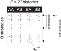
Figure 3: Stylistic example of the $m=2$ strategy space.

The collection of all possible strategies (and their associated virtual points) is hereafter referred to as the strategy space, see e.g. Figure 3. This object can be thought of as a common property of the game itself, being updated centrally after each timestep. Each individual agent monitors only a fixed subset $q$ of the $Q$ possible strategies (with the small caveat that a repeated strategy choice is possible). After each turn, an agent assigns one (virtual) point to each of its strategies which would have predicted the correct outcome. The virtual points for each strategy can be represented by the strategy score vector $\mathbf{S}(t)$, and are given by

$$\mathbf{S}(t) = \sum_{i=t-T}^{t-1}\mathbf{a}^{\mu(i)}\chi\Big{[}N_{A}(i),L(i)\Big{]}$$ (4)

In total, there are $Q=2^{P}$ possible strategies which define the decisions in response to all possible $m$ history bit-strings. This is referred to as the full strategy space (FSS). However, the principal features of the system are reproduced in a smaller reduced strategy space (RSS) of $Q=2^{m+1}$ strategies wherein any two strategies are either un-correlated or anti-correlated [6], i.e. separated by a Hamming distance of either $2^{m}$ or $2^{m-1}$. The full and reduced strategy space $\mathbf{a}$ for $m=2$ has been reproduced in Figure 4. Each row represents a strategy, each column is assigned to a particular history, giving the strategy space a dimension of $P\times Q$. The prediction of strategy $R$ to information $\mu$ is $a^{\mu}_{R}$ and corresponds to the $(R,\mu)$ element of $\mathbf{a}$. The ordering of the rows in unimportant.

$$\mathbf{a}=\begin{pmatrix}-1&-1&-1&-1\\ -1&-1&-1&1\\ -1&-1&1&-1\\ -1&-1&1&1\\ -1&1&-1&-1\\ -1&1&-1&1\\ -1&1&1&-1\\ -1&1&1&1\\ 1&-1&-1&-1\\ 1&-1&-1&1\\ 1&-1&1&-1\\ 1&-1&1&1\\ 1&1&-1&-1\\ 1&1&-1&1\\ 1&1&1&-1\\ 1&1&1&1\end{pmatrix}\qquad\mathbf{a}=\begin{pmatrix}-1&-1&-1&-1\\ -1&1&-1&1\\ 1&1&-1&-1\\ 1&-1&-1&1\\ 1&1&1&1\\ 1&-1&1&-1\\ -1&-1&1&1\\ -1&1&1&-1\\ \end{pmatrix}$$

Figure 4: Example of an $m=2$ strategy space. The full strategy space containing 16 strategies is reproduced on the left, with the reduced strategy space of 8 strategies on the right.

Within the strategy space, each strategy $R$ has an anticorrelated strategy $\bar{R}$. We note that the anticorrelated strategies are effectively redundant, as their predictions and strategy scores can be recovered from their anticorrelated pair:

$$\mathbf{a}_{\bar{R}}^{\mu} = -\mathbf{a}_{R}^{\mu},$$ (5a)

$$\mathbf{S}_{\bar{R}}(t) = -\mathbf{S}_{R}(t).$$ (5b)

Equation (5a) is true by definition, i.e. a strategy and its anticorrelated pair always give the opposite prediction. However (5b) requires a symmetric scoring rule to be used, which is satisfied by (1). Thus we can reproduce the dynamics using a space of just $P$ strategies, in which agents choose both a strategy and whether to agree or disagree with its prediction. Reducing the size of the strategy space is advantageous as it reduces memory requirements and increases the speed of the simulation. For a more detailed description of how to implement such a system, see [22].

3 Demonstration of large changes

A ubiquitous feature of complex systems is that large changes, or ‘extreme events’, arise far more often than would be expected if the individual agents acted independently. We frequently refer to crashes, but are interested in large moves in either direction. With a suitable choice of parameters the GCBG is able to generate time series which include occasional large movements, see e.g. Figure 5. The game can be broadly classified into three regimes:

1. The number of strategies in play is much greater than the total available: groups of traders will play using the same strategy and therefore crowds should dominate the game [19].

2. The number of strategies in play is much less than the total available: grouping behaviour is therefore minimal.

3. The number of strategies in play is comparable to the total number available.

We focus on the third regime, since this yields seemingly random dynamics with occasional large movements.

Large changes seem to exhibit a wide range of possible durations and magnitudes making them difficult to capture using traditional statistical techniques based on one or two-point probability distributions. A common feature, however, is an obvious trend (i.e. to the eye) in one direction over a reasonably short time window: we use this as a working definition of a large change. (In fact, all the large changes discussed here represent $>3\sigma$ events.) In both our model and the real-world system, these large changes arise more frequently than would be expected from a random-walk model [18].

In §3.1 we consider the distribution of the excess demand created by our generic system, and perform a simple analysis to discuss the statistics of extreme events. To determine whether large movements occur due to a single random event, we examine the stochastic influence present within the model in §3.2 and find that they arise through a global cooperation occurring over the whole system.

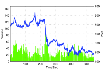
Figure 5: Example of a time series exhibiting large changes. The model parameters were $N_{tot}=101$, $T=60$, $\tau=0.53$, $m=3$ and $q=2$.

3.1 Tail estimation

Traditional parametric statistical methods are ill-suited for dealing with extreme events, which have little historical data associated with them. Provided the distribution has a finite variance and the increments are independent, the Central Limit Theorem will apply near the centre of the distribution, but does not tell us anything about the tails [4]. In recent years extreme value theory (EVT), a branch of probability theory which focuses explicitly on extreme outcomes, has received increasing attention [10]. EVT considers the distribution of extreme returns rather than the distribution of all returns. It can be shown that the limiting distribution of extreme returns observed over a long time-period is largely independent of the distribution of returns itself. The upper tail of a fat-tailed cumulative distribution function $F$ behaves asymptotically like the tail of the Pareto distribution given by $1-F(x)\approx cx^{-\alpha}$, for $c>0$, $\alpha>0$ and $x\geq C$, where $C$ is a threshold above which the assumed algebraic form is valid, and $c$ is a normalising constant. The tail index $\alpha$ determines the heaviness of the tail of a distribution and plays a key role in tail-related risk measures, representing the maximal order of finite moments. Only the first $k$ moments, where $k<\alpha$, are bounded. The greater the tail index, the ‘fatter’ the tail, and the greater the incidence of extreme events.

An important issue in the study of fat-tailed distributions is the estimation of the tail index $\alpha$. There are a number of methods to estimate the tail index, some using asymptotic results from EVT, from which values can be estimated using maximum likelihood techniques. However the Hill estimator is commonly used, as it is suitable for tail estimation of fat-tailed distributions and is relatively easy to implement [14]. Consider a sample $X_{1},X_{2},\ldots,X_{n}$ of $n$ observations drawn from a stationary iid process, and let $X_{(1)}\geq X_{(2)}\geq\ldots\geq X_{(n)}$ be the descending order statistics. The Hill estimator is based on the difference between the $m$th largest observation and the average of the $m$ largest observations:

$$\hat{\xi}_{m} = \frac{1}{m}\sum_{i=1}^{m}\log X_{(i)}-\log X_{(m)}$$

where $\xi=1/\alpha$ is the shape parameter and $m$ is the number of order statistics used in the tail estimation. The appropriate choice of value $m$ is a non-trivial problem, since this requires us to decide where the tail begins. There is a tradeoff between the bias and variance of the estimator in choosing $m$. If we choose a large value of $m$, the number of order statistics used increases and the variance of the estimator will decrease. However, choosing a high $m$ also introduces some observations from the centre of the distribution and the estimation becomes biased. But if it is too small, the estimate will be based on a just a few of the largest observations and the estimator will lack precision. Several methods for the determination of an optimal sample fraction for the Hill estimator have been proposed [7, 9]. In Figure 6 a Hill plot is constructed from the simulation data used to create Fig. 5. A threshold is selected from the plot where the shape parameter is fairly stable, giving an estimate of the tail index $\alpha\approx 3.7$. To obtain the most accurate tail estimate, a combination of several techniques should be considered.

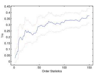
Figure 6: Hill-plot with a 0.95 confidence interval. The estimated value of the shape parameter $\xi$ is plotted against the number of upper order statistics $m$ used in the estimation. A value of $\xi$ is selected from the plot where the shape parameter is fairly stable

3.2 The effect of stochasticity

To investigate the stochastic influence due to the effect of coin tosses, we have studied their occurrence during the simulation. We define two types of coin toss: type (i), which occurs when an agent has a tie between active strategy options which predict differing outcomes, and type (ii), which occurs when the number of agents choosing option A is equal to the number choosing option B. The main conclusion is that there is no single-coin toss that immediately causes a large change within the system. and The large movements observed as arising endogenously in the system, result from the organisation of temporal and spatial (i.e. strategy space) correlations. In common with other complex adaptive systems, this organisation does not arise in general from a nucleation phase diffusing across the system, e.g. it cannot be traced to a particular coin-toss by a particular agent which triggers the “avalanche”. Rather, it results from a progressive and more global cooperation occurring over the whole system via repetitive interactions [27].

4 A study of extreme events

In this section we consider the generic complex system introduced in §2 in which a population of $N_{tot}$ heterogeneous agents with limited capabilities and information, repeatedly compete for a limited global resource. We focus on extreme events which are endogenous (i.e. internally-produced by the agents themselves) and provide a microscopic understanding as to their build-up and likely duration.

4.1 Nodal weight decomposition

The dynamics of the game history can be usefully represented on a directed de Bruijn graph [23]. This is a graph whose nodes are sequences of symbols from some alphabet, and whose edges represent possible transitions between these nodes. It has numerous interesting properties and is frequently discussed in the context of parallel algorithms and communications networks. This is an effective method of representing the evolution of the system, and in Figure 7 we plot the de Bruijn graph for an $m=3$ game.

Large changes occur when connected nodes become persistent and the game makes successive moves in the same direction. Only nodes 0 and 7 can exhibit perfect nodal persistence, where an allowed transition can return the system to exactly the same node. This is the simplest type of large change, e.g. $\mu(t)=0,0,0,0,\ldots$, where all successive price changes are in the same direction. We call this a ‘fixed-node crash’ (or rally). There are many other possibilities reflecting the wide range of forms and durations that a large change can undertake. For example, on the $m=3$ de Bruijn graph in Fig. 7 the cycle $\mu=0,0,1,2,4,0,\ldots$ has four out of the five transitions producing price-changes of the same sign (it is persistent on nodes 1, 2, 4 and antipersistent on node 0). We call this a ‘cyclic-node crash’. Stable behaviour occurs on a path where all transitions are equally visited, e.g. $\mu(t)=0,0,1,3,6,5,3,7,7,6,4,1,2,5,4,\ldots$.

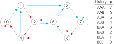
Figure 7: Dynamical behaviour of the global information is described by transitions on the de Bruijn graph. Graph for population of $m=3$ agents. Blue transitions represent positive demand $D$, red transitions represent negative demand, with each transition incurring an increment to the score vector $\mathbf{S}$.

To identify moments when large changes occur, we need to recognise when history nodes are likely to become persistent. Whether a node is persistant or not will depend on the action of the agents at that timestep, which is determined by the predictions of the strategies they hold. If the majority of active strategies generate a prediction of the same outcome, then the demand at that timestep is likely to continue in that direction. Thus a suitable condition for a large movement is when there is a concensus of opinion regarding the next outcome amongst the active strategies. This occurs when the pattern of active strategies within the strategy space matches up with the pattern of stratgy predictions for a history node $\mu$, see Figure 8. The strategy predictions will depend on the global information $\mu(t)$, and the distribution of active strategies depends on the strategy score vector $\mathbf{S}(t)$. At each timestep $\mathbf{S}(t)$ is updated according to whether a strategy predicted the winning outcome $w(t)$; the incremental strategy score is given by a column of the strategy matrix $\mathbf{a}$ determined by $\mu(t)$. In total there are $P$ orthogonal increment vectors $\mathbf{a}^{\mu}$, one for each value of $\mu$. We can express the strategy score (4) as

$$\mathbf{S}(t)=c_{0}\mathbf{a}^{0}+c_{1}\mathbf{a}^{1}+\ldots+c_{P-1}\mathbf{a}^{P-1}\ =\ \sum_{j=0}^{P-1}c_{j}\mathbf{a}^{j},$$ (6)

where $c_{j}$ represents the nodal weight for history node $\mu=j$. The nodal weights represent the number of negative return transitions from node $\mu$ minus the number of positive return transitions, in the time window $t-T\rightarrow t-1$. The values of these nodal weights are important in identifying periods in which large changes can occur. If the value of a nodal weight is near zero, this implies that the number of active strategies predicting outcome A will be similar to the number predicting outcome B when that node is reached. The excess demand will then depend on the quenched disorder and the undecided agents, but is likely to be small. Conversely, if the value of a nodal weight is significantly different from zero, this indicates a bias in the strategy space, i.e. the same pattern is evident in the active strategies and the strategy predictions. When the game trajectory hits this node, the majority of active strategies will predict the same outcome, and there will be a consensus amongst the agents. This is likely to lead to a large excess demand, and therefore a large change. Thus high absolute nodal weight implies persistence in transitions from that node, i.e. persistence in $D|\mu$.

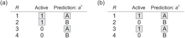
Figure 8: Two different configurations of the strategy space for $\mu(t)=0$. The columns represent: $R$ – strategy index; Active – where ‘1’ represents an active strategy and ‘0’ an inactive strategy, i.e. ${\cal H}[S_{R}(t)-r]$; Prediction – the prediction of the strategy, which is given by $a^{0}_{R}$. In (a) there is no consensus in the predictions of the active strategies. The active strategies do not share the same pattern as $\mathbf{a}^{0}$. In (b) there is a consensus of opinion. All the active strategies predict option $A$ since the pattern of active strategies is similar to the pattern of strategy predictions.

The mean of the strategy scores predicting an $A$ or $B$ at node $\mu$ are linked to their nodal weight:

$$\mbox{E}\left[S_{R\ni a_{R}^{\mu}=1}(t)\right] = c_{\mu}(t),$$ (7a)

$$\mbox{E}\left[S_{R\ni a_{R}^{\mu}=-1}(t)\right] = -c_{\mu}(t).$$ (7b)

This symmetry occurs because each strategy has an anticorrelated strategy present in the strategy space.

The nodal weight decomposition provides a succinct method of describing the state of the strategy space. We are concerned with high nodal weights on game cycles that can become persistent. When a nodal weight value becomes large, this is a warning sign that the system is in a suitable state to undergo a large change. Figure 9 illustrates a large change which starts as a fixed-node crash, and then subsequently becomes a cyclic-node crash.

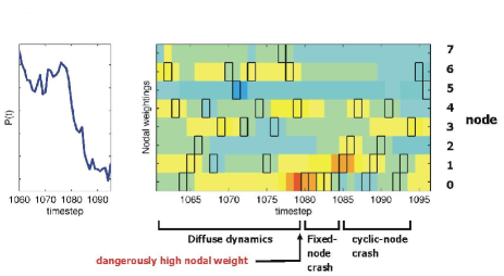
Figure 9: Dynamical behaviour of complex system (e.g. price $P(t)$ in financial market) described by evolution of nodal weights $c_{\mu}$. History at each timestep indicated by black square. Large change preceded by abnormally high nodal weight. Large change incorporates fixed-node and cyclic node crashes.

4.2 Estimating the crash length

We are interested in the dynamics of large changes, and use a simplified version of the system to obtain an analytic expression for the expected crash length. Reference [15] showed that the GCBG can be usefully described as a stochastically disturbed deterministic system. As stated in (3), the demand can be divided into contributions arising from agents acting on a definite strategy $D_{D}(t)$, and that from the undecided agents $D_{U}$. The average contribution of the undecided agents to the net demand will be zero, i.e. $\mbox{E}[D_{U}(t)]=0$. Averaging over our model’s stochasticity in this way yields a description of the game’s deterministic dynamics. By examining these dynamics, we can determine when a large-change is likely. For $q=2$ the demand function can be expressed as

$$D(t) = \sum_{R=1}^{Q}a_{R}^{\mu(t)}{\cal H}[S_{R}(t)-r]\sum_{R^{\prime}=1}^{Q}\left(1+\mbox{sgn}\left[S_{R}(t)-S_{R^{\prime}}(t)\right]\right)\Psi_{R,R^{\prime}},$$ (8)

where $\mathbf{\Psi}$ is the symmetrized strategy allocation matrix which constitutes the quenched disorder present during the system’s evolution. The volume $V(t)$ is given by the same expression as $D(t)$ replacing $a_{R}^{\mu(t)}$ by unity.

For the parameter ranges of interest, the choice about whether a strategy is played by an agent is more determined by whether that strategy’s score is above the threshold, than whether it is their highest-scoring strategy. This is because agents are only likely to have at most one strategy whose score lies above the threshold for confidence levels $r\geq 0$. Making the additional numerically-justified approximation of small quenched disorder (i.e. the variance of the entries in the strategy allocation matrix $\mathbf{\Psi}$ is smaller than their mean for the parameter range of interest [15]), the demand and volume become

$$D(t) = \sum_{R=1}^{Q}a_{R}^{\mu(t)}{\cal H}[S_{R}(t)-r]\sum_{R^{\prime}=1}^{Q}\frac{N}{Q^{2}}$$ (9a)

$$= \frac{N}{Q}\sum_{R=1}^{Q}a_{R}^{\mu(t)}{\cal H}\left[S_{R}(t)-r\right]$$

$$= \frac{N}{Q}\sum_{R=1}^{Q}a_{R}^{\mu(t)}\frac{1}{2}\Big{(}1+\mbox{sgn}\left[S_{R}(t)-r\right]\Big{)}$$

$$= \frac{N}{2Q}\sum_{R=1}^{Q}a_{R}^{\mu(t)}\mbox{sgn}\left[S_{R}(t)-r\right],$$

$$V(t) = \frac{N}{Q}\sum_{R=1}^{Q}{\cal H}\left[S_{R}(t)-r\right]\ =\ \frac{N}{2}+\frac{N}{2Q}\sum_{R=1}^{Q}\mbox{sgn}\left[S_{R}(t)-r\right].$$ (9b)

Let us suppose persistence on node $\mu=0$ starts at time $t_{0}$. How long will the resulting large change last? To answer this, we decompose (9a) into strategies which predict option $A$ at $\mu=0$, and those that predict $B$. We first consider the particular case where the node $\mu=0$ was not visited during the previous $T$ timesteps, hence the loss of score increment from time-step $t-T$ will not affect $\mathbf{S}(t)$ on average. At any later time $t_{0}+\tau$ during the large change, (9a) and (9b) are given by

$$D(t_{0}+\tau) = -\frac{N}{2Q}\left\{\sum_{R\ni a_{R}^{\mu}=-1}\operatorname*{sgn}\left[S_{R}(t_{0})-r-\tau\right]-\sum_{R\ni a_{R}^{\mu}=1}\operatorname*{sgn}\left[S_{R}(t_{0})-r+\tau\right]\right\},$$ (10)

$$V(t_{0}+\tau) = \frac{N}{2}+\frac{N}{2Q}\left\{\sum_{R\ni a_{R}^{\mu}=-1}\operatorname*{sgn}\left[S_{R}(t_{0})-r-\tau\right]+\sum_{R\ni a_{R}^{\mu}=1}\operatorname*{sgn}\left[S_{R}(t_{0})-r+\tau\right]\right\}.$$

The magnitude of the demand $|D(t_{0}+\tau)|$ decreases as the persistence time $\tau$ increases, and the large change will end at time $t_{0}+\tau_{c}$ when the right-hand side of (10) becomes zero. We denote the persistence time or ‘crash-length’ by $\tau_{c}$. It is easy to obtain an upper limit for the duration of a large change by determining when the demand $D$ changes sign. This occurs when the mean of the scores of the strategies predicting $A$ returns to 0, i.e.

$$\tau_{c} = \mbox{E}\left[S_{R\ni a_{R}^{\mu}=-1}(t_{0})\right]$$

$$= -c_{0}(t_{0})$$

from (7b). Thus the crash length will depend on the score difference between strategies predicting option $A$ and those predicting $B$. In the more general case, where the node $\mu=0$ was visited during the previous $T$ timesteps, $\tau_{c}$ is given by the largest $\tau$ value which satisfies

$$\tau = -\left(c_{0}(t_{0})+\sum_{\{t^{\prime}\}}\operatorname*{sgn}\left[D(t^{\prime})\right]\right)$$ (11)

where $\{t^{\prime}\}\ni(\mu(t^{\prime})=0\cap t_{0}-T\leq t^{\prime}\leq t_{0}-T+\tau)$. The summation accounts for any $\mu=0$ transitions in the period $t_{0}-T$ to $t_{0}-T+\tau$.

To obtain an improved estimate of $\tau_{c}$, and investigate the behaviour of the demand and volume, it is necessary to assume a distribution for the strategy scores. In Figure 10 we plot an example of the strategy score distribution prior to a large change. We assume that the scores have a near-Normal distribution, i.e. $S_{R\ni a_{R}^{\mu}=-1}(t_{0})\sim\operatorname*{N}[-c_{0}(t_{0}),\sigma]$ as shown Fig. 11. Consequently, prior to a large change, the score distribution tends to split into two halves. Substitution into (10) gives the expected demand and volume during the crash:

$$D(t_{0}+\tau) \propto \Phi\left[\frac{c_{0}(t_{0})-r+\tau}{\sigma}\right]-\Phi\left[\frac{-c_{0}(t_{0})-r-\tau}{\sigma}\right],$$

$$V(t_{0}+\tau) \propto \Phi\left[\frac{c_{0}(t_{0})-r+\tau}{\sigma}\right]+\Phi\left[\frac{-c_{0}(t_{0})-r-\tau}{\sigma}\right].$$

These forms are illustrated in Figure 12. As the spread in the strategy score distribution is increased, the dependence of $D$ and $V$ on the parameters $\tau$ and $r$ becomes weaker and the surfaces flatten out leading to a smoother drawdown, as opposed to a sudden severe crash. In the limit $\sigma\rightarrow 0$, the crash-length $\tau_{c}=-c_{0}(t_{0})-|r|$. As the parameters $c_{0},\sigma,r$ are varied, it can be seen that the behaviour of the demand and volume during the large change can exhibit markedly different qualitative forms.

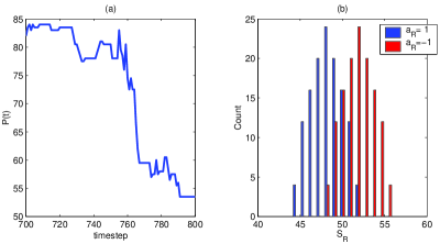
Figure 10: Empirical strategy score distribution. (b) is the strategy score distribution at timestep 760 from the series depicted in (a).

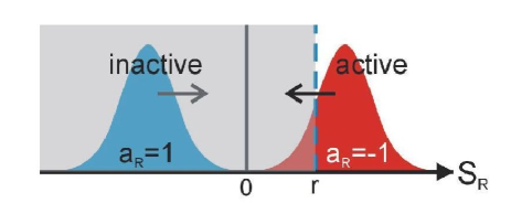
Figure 11: Schematic representation of strategy score distribution prior to crash. Arrows indicate subsequent motion during crash period.

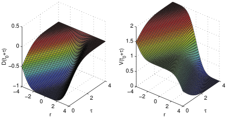
Figure 12: Plots of expected demand $D(t)$ and volume $V(t)$ during crash period showing range of different possible behaviour as system parameters are varied.

4.3 Repeated occurence of large changes

We now turn to the important practical question of whether history will repeat itself, i.e. given that a large change has recently happened, is it likely to happen again? If so, is it likely to be even bigger? Suppose the system has built up a negative nodal weight for $\mu=0$ at some point in the game (see Fig. 13a). It then hits node $\mu=0$ at time $t_{0}$ producing a large change (Fig. 13b). The nodal weight $c_{0}$ is hence restored to zero (Fig. 13c). In this model the previous build-up is then forgotten because of the finite $T$ score window, hence $c_{0}$ becomes positive (Fig. 13d). The system then corrects this imbalance (Fig. 13e), restoring $c_{0}$ to 0. The large change is then forgotten, hence $c_{0}$ becomes negative (Fig. 13f). The system should therefore crash again - however, a crash will only re-appear if the system’s trajectory subsequently returns to node $\mu=0$. Interestingly, we find that the disorder in the initial distribution of strategies among agents (i.e. the quenched disorder in $\mathbf{\Psi}$) can play a deciding role in the issue of ‘births and revivals’ of large changes since it leads to a slight bias in the outcome, and hence the subsequent transition, at each node. In certain configurations, this system may demonstrate repeated instabilities leading to large changes. When $c_{\mu(t)}=0$ (see Fig. 13c), it follows that $\operatorname*{sgn}[D(t)]$ is more likely to be equal to $\operatorname*{sgn}\left[\mathbf{a}^{\mu(t)}\cdot\mathbf{x}\right]$ where $x_{R}=\sum_{R^{\prime}}\Psi_{R,R^{\prime}}$ is a strategy weight vector with $x_{R}$ corresponding to the number of agents who hold strategy $R$ [16]. The quenched disorder therefore provides a crucial bias for determining the future trajectory on the de Bruijn graph when the nodal weight is small, and hence can decide whether a given large change recurs or simply disappears. The quenched disorder also provides a catalyst for building up a very large change [16].

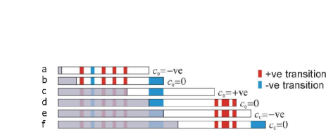
Figure 13: Representation of how large changes can recur due to finite memory of agents. Grey area shows history period outside agents’ memory. Example shows recurring fixed-node crash at node $\mu=0$.

5 Concluding remarks

We have addressed the issue of understanding, predicting and eventually controlling catastrophic endogenous changes in a collective. By utilizing information about the strategy weights within the model, we have developed a method for determining when a large change is likely within a generic complex system, the so-called GCBG, and obtained an analytic expression for its expected duration. Our work opens up the study of how a ‘complex-systems-manager’ might use this information to control the long-term evolution of a complex system by introducing, or manipulating, such large changes [16]. As an example, we give a quick three-step solution to prevent large changes: (1) use the past history of outcomes to build up an estimate of the score vector $\mbox{S}(t)$ and the nodal weights $\{c_{\mu(t)}\}$ on the various critical nodes, such as $\mu=0$ in the case of the fixed-node crash. (2) Monitor these weights to check for any large build-up. (3) If such a build-up occurs, step in to prevent the system hitting that node until the weights have decreased. Finally we note that it can sometimes be beneficial to induce small changes ahead of time, in order to avoid larger changes in the future. We call this process ‘immunization’ and refer to Ref. [12] for more details.

We are grateful to David Wolpert, Kagan Tumer and Damien Challet for many useful discussions about Collectives.

References

- [1] W. Brian Arthur. Bounded rationality and inductive behavior (the El Farol problem). The American Economic Review, 1994.
- [2] Per Bak. How Nature Works: The Science of Self-Organised Criticality. Oxford University Press, Oxford, 1997.
- [3] G. Boffetta, M. Cencini, M. Falcioni, and A. Vulpiani. Predictability: a way to characterize complexity. Physics Reports, 356:367–474, 2002.
- [4] Jean-Philippe Bouchaud and Marc Potters. Theory of Financial Risks. Cambridge University Press, Cambridge, 2000.
- [5] Damien Challet and Yi-Cheng Zhang. Emergence of cooperation and organization in an evolutionary game. Physica A, 246(3-4):407–418, 1997.
- [6] Damien Challet and Yi-Cheng Zhang. On the minority game: Analytical and numerical studies. Physica A, 256(3-4):514–532, 1998.
- [7] J. Danielsson, L. de Haan, L. Peng, and C. G. de Vries. Using a bootstrap method to choose the sample fraction in tail index estimation. Journal of Multivariate Analysis, 76:226–248, 2001.
- [8] Mark d’Inverno and Michael Luck, editors. The Fourth UK Workshop on Multi-Agent Systems, December 2001.
- [9] Holger Drees and Edgar Kaufmann. Selecting the optimal sample fraction in univariate extreme value estimation. Stochastic Processes and their Applications, 75:149–172, 1998.
- [10] Paul Embrechts, Claudia Klüppelberg, and Thomas Mikosch. Modelling Extremal Events for Insurance and Finance. Springer, London, 1999.
- [11] Michael L. Hart, Paul Jefferies, and Neil F. Johnson. Dynamics of the time horizon minority game. cond-mat/0102384, December 2001.
- [12] Michael L. Hart, David Lamper, and Neil F. Johnson. An investigation of crash avoidance in a complex system. cond-mat/0207588. See also Physica A, in press (2002).
- [13] Richard A. Heath. Can people predict chaotic sequences. Nonlinear Dynamics, Psychology, & Life Sciences, 6:37–54, 2002.
- [14] B.M. Hill. A simple general approach to inference about the tail of a distribution. Annals of Statistics, 46:1163–1173, 1975.
- [15] Paul Jefferies, Michael L. Hart, and Neil F. Johnson. Deterministic dynamics in the minority game. Physical Review E, 65(016105), 2002.
- [16] Paul Jefferies, David Lamper, and Neil F. Johnson. Anatomy of extreme events in a complex adaptive system. cond-mat/0201540.
- [17] Nicholas R. Jennings and Yves Lespérance, editors. Intelligent Agents VI, number 1757 in Lecture Notes in Computer Science. Springer, 2000.
- [18] Anders Johansen and Didier Sornette. Large stock market price drawdowns are outliers. Journal of Risk, 4(2), 2002.
- [19] Neil F. Johnson, Michael L. Hart, and Pak Ming Hui. Crowd effects and volatility in markets with competing agents. Physica A, 269(1):1–8, 2000.
- [20] Neil F. Johnson, Michael L. Hart, Pak Ming Hui, and Dafeng Zheng. Trader dynamics in a model market. International Journal of Theoretical and Applied Finance, 3(4):443–450, 2000.
- [21] David Lamper, Sam H. Howison, and Neil F. Johnson. Predictability of large future changes in a competitive evolving population. Physical Review Letters, 88(017902), 2002.
- [22] David Lamper and Neil F. Johnson. Complexity. forthcoming in Dr Dobb’s Journal, 2002.
- [23] Richard Metzler. Antipersistant binary time series. Journal of Physics A, 35(3):721–730, 2002.
- [24] Paul Ormerod. Surprised by depression. Finanical Times, page 25, February 19 2001.
- [25] Complex systems. Science, 284(5411), 1999.
- [26] Michael F. Shlesinger. Comment on “Stochastic process with ultraslow convergence to a gaussian: The truncated Levy flight”. Physical Review Letters, 74(24):4959, 1995.
- [27] Didier Sornette. Critical Phenomena in Natural Sciences. Springer, New York, 2000.
- [28] Michael Wooldridge and Nicholas R. Jennings. Intelligent agents: Theory and practice. Knowledge Engineering Review, 10(2), June 1995.
- [29] D.H. Wolpert, K. Wheeler and K. Tumer. Collective intelligence for control of distributed dynamical systems). Europhysics Letters, 49:March 2000.
- [30] Karl Ziemelis. Complex systems. Nature, 410, March 2001.