1 Introduction

In 1918 Schottky discovered that the fluctuations in vacuum diodes can be related to the discrete nature of the charge carriers [1]. His observation was that the power spectrum of the current fluctuations gave direct access to the charge $e$ of the discrete carriers responsible for the current. From his theoretical considerations he found a relation between the noise power of the current fluctuations $S_{I}$ and the average current $I$,

$$S_{I}=2eI\,,$$ (1)

a result nowadays known as the Schottky formula. Its consequence is, that the current noise provides information on the transport process, which is not accessible through conductance measurements only.

Studies of the noise properties of tunnel-junctions renewed the interest in noise later [2]. Since about ten years the investigation of transport in quantum coherent structures has boosted the interest in the theory of current noise in mesoscopic structures [3, 4]. Correlations in the transport of fermions have lead to a number of interesting predictions. For example, the noise of a single channel quantum contact of transparency $T$ at zero temperature has the form $S_{I}=2eI(1-T)$ [5, 6]. The noise is thus suppressed below the Schottky value, Eq. (1). The suppression is a direct consequence of the Pauli principle, and is therefore specific to electrons. Particles with bosonic statistics or classical particles show a different behaviour, e. g. for Bosons the noise is enhanced by a factor $1+T$. A convenient measure of the deviation from the Schottky result is the so-called Fano factor $F=S_{I}/2eI$. For a number of generic conductors, it turns out that the suppression of the Fano factor is universal, i. e. it does not depend on details of the conductor like geometry or impurity concentration. A diffusive metal with purely elastic scattering leads to $F_{diff}=1/3$ [7, 8], which is independent on the concrete shape of the conductor [9]. In a symmetric double tunnel junction, on the other hand, $F_{dbltun}=1/2$ [10]. A chaotic cavity (a small region with classical chaotic dynamics, connected to two leads by open quantum point contacts) shows a suppression of $F_{cavity}=1/4$ [11]. Thus, we conclude that from a noise measurement two kinds of information can be obtained. First, we can get information on the statistics of the carriers, e. g. if they are fermions. Second, provided the statistics is known, the comparison of the magnitude of the noise power with the average current gives information on the internal structure of the system. However, the picture described here is a little bit too simplified. In many real experiments the structure is much less well defined, the temperature is finite, or other complications make the interpretation of experimental data less trivial.

Having motivated the interest in the noise, we may ask, what we can learn further from current fluctuations. Higher correlators of the current will provide even more information on the transport process. However, theoretical calculations of higher correlators become increasingly cumbersome and one should find a different concept to obtain this information. This step was performed by a transfer of concepts from the field of quantum optics. Here it is possible to count experimentally the number of photons occupying a certain quantum state. This number is subject to quantum and thermal fluctuations and requires a statistical description: the full counting statistics (FCS). Lesovik and Levitov adopted this terminology to mesoscopic electron transport [12, 13], in which the electrons passing a certain conductor are counted. Since then the FCS has been studied in the field of mesoscopic electron transport. It the aim of this article to review some of the progress, which has been recently made.

The general problem of counting statistics has been considered before on a heuristic level. If one makes the ad hoc assumption that individual transfers of charges are uncorrelated and unidirectional, simple calculation show that the probability distribution of the number of transfered charges is Poissonian

$$P_{t_{0}}(N)=e^{-\bar{N}(t_{0})}\frac{{\bar{N}(t_{0})}^{N}}{N!}\,.$$ (2)

Here $t_{0}$ is the time period during which the charges are counted and $\bar{N}(t_{0})=It_{0}/e$ is the average number of transfered charges. Schottky’s result (1) for the current noise power can be easily derived from Eq. (2). This kind of counting statistics is usually found in tunnel junctions, where the charge transfers are rare events, or at high temperatures, when the mean occupation of the states is small and the statistics of the particles plays no role. However, in a degenerate electron gas one encounters a completely different situation: all states are filled due to Fermi correlations. If we now consider a quantum transport channel of transmission probability $T$ and applied bias voltage $V$, the rigidity of the Fermi sea leads to a fixed number of electrons, which are sent into each quantum channel. A charge is transfered to the other side with probability $T$ and the statistics is therefore binomial

$$P_{t_{0}}(N)={M(t_{0})\choose N}T^{N}(1-T)^{M(t_{0})-N}\,.$$ (3)

This is the result of the quantum calculation of Levitov and coworkers [12]. Note, that arguments based on the FCS have been used already to interpret current noise calculations or measurements. However, in general these interpretations are not unique, and a calculation of the FCS is required to interpret the results for the noise unambiguously. Thus, obtaining the FCS is a theoretical task, which leads to a better understanding of quantum transport processes.

The structure of this article is as follows. In the next section we introduce the theoretical basis, necessary to obtain the FCS. Our approach is based on an extension of the well-known Keldysh-Green’s function technique [14] and described in Section 2.2. A convenient simplification is the circuit theory of mesoscopic transport, developed by Nazarov [15], which allows to obtain the FCS for a large variety of multi-terminal structures with minimal calculational overhead. In the two following sections, we will discuss several concrete examples. First, we show that for phase coherent two-terminal conductors the counting statistics can be obtained in quite a general form [16]. This is illustrated for normal and superconducting constrictions as well as two-barrier structures. A somewhat special case is the diffusive conductor coupled to a superconductor (i. e. in the presence of proximity effect), where intrinsic decoherence between electrons and holes influences the transport properties [17]. Second, we turn to more complex mesoscopic structures with more than two terminals. An analytic solution is obtained for the case of an arbitrary number of terminal connected by tunnel junctions to one central node [18]. As specific example we calculate the counting statistics of a beam splitter, in which a normal current or a supercurrent is divided into two normal currents. Afterwards we present some conclusions. In the appendices we give some theoretical background information to the methods used in this article.

In this article we concentrate on counting statistics in two- or multi-terminal devices with either normal- or superconducting contacts. More aspects of FCS are in other parts of this book. We would like to mention works related to FCS not covered here. Normal-superconductor transport at finite energies and magnetic fields was recently addressed in [19, 20]. Time-dependent transport phenomena in normal contacts have been studied in [13]. Fluctuations of the current in adiabatic quantum pumps have attracted some attention (see e.g. [21]). A connection to photon counting or photon transport can be found in Refs. [22, 23]. Counting statistics has also been addressed in the context of the readout process of a qubit [24] or to study spin coherence effects [25]. Results for the FCS of entangled electron pairs [26] and of resonant Cooper pair tunneling [27] have also been published.

2 Counting Statistics and Green’s function

2.1 Basics of Current Statistics

We introduce some basic formulas, relevant for the theory of FCS. The quantity we are after is the probability $P_{t_{0}}(N)$, that $N$ charges are transfered in the time interval $t_{0}$. Equivalently, we can find the cumulant generating function (CGF) $S(\chi)$, defined by

$$\exp(-S(\chi))=\sum_{N}P_{t_{0}}(N)\exp(iN\chi)\;.$$ (4)

To keep notations simple in this section, we will limit the discussion to the two-terminal case, in which only the number $N$ of transfered charges in one terminal matters. In the other terminal it is given by $-N$, since the total number of charges is conserved. However, most relations are straightforwardly generalized to many terminals. Note that normalization of the FCS requires that $S(0)=0$. Also, we will suppress the explicit dependence of $S(\chi)$ on the measuring time $t_{0}$. In the static case considered mostly in this article, we have $S(\chi)\sim t_{0}$.

From the full counting statistics one obtains the cumulants

$$C_{1}=\overline{N}\equiv\sum_{N}NP_{t_{0}}(N) C_{2}=\overline{(N-\overline{N})^{2}}\,,$$ , (5)

$$C_{3}=\overline{(N-\overline{N})^{3}} C_{4}=\overline{(N-\overline{N})^{4}}-3\overline{(N-\overline{N})^{2}}^{2}\,,$$ , (6)

and so on. The meanings of the various cumulants are depicted in Fig. 1a. Alternatively, the cumulants can be obtained from the CGF

$$C_{n}=-\left.\left(-i\right)^{n}\frac{\partial^{n}}{\partial\chi^{n}}S(\chi)\right|_{\chi=0}\;.$$ (7)

The relation to the average current and the noise power of current fluctuations is obtained as follows. Almost trivially one has

$$C_{1}=\langle N\rangle=\frac{1}{-e}\int_{0}^{t_{0}}dt\langle I(t)\rangle=-\frac{t_{0}}{e}\bar{I}\,,$$ (8)

where we have denoted the charge of the electrons with $-e$. The relation between the second cumulant and the current noise power

$$S_{I}\equiv\int_{-\infty}^{\infty}d\tau\left\langle\left\{\delta I(\tau),\delta I(0)\right\}\right\rangle$$ (9)

is less obvious. We write for the second cumulant

$$C_{2}=\overline{(N-\overline{N})^{2}}=\frac{1}{2e^{2}}\int_{0}^{t_{0}}\int_{0}^{t_{0}}dtdt^{\prime}\langle\{\delta I(t),\delta I(t^{\prime})\}\rangle\,,$$ (10)

where $\delta I(t)=I(t)-\langle I\rangle$ is the current fluctuation operator and $\langle...\rangle$ denote the quantum statistical average. We transform the time coordinates to average $\overline{t}=(t+t^{\prime})/2$ and relative time $\tau=t-t^{\prime}$. Assuming the observation $t_{0}$ is much larger than the correlation time of the currents, the correlator in Eq. (10) does not depend on $T$, and we find the desired relation between current noise power and the second cumulant

$$S_{I}=\frac{2e^{2}}{t_{0}}\left.\frac{\partial^{2}S(\chi)}{\partial\chi^{2}}\right|_{\chi=0}\,.$$ (11)

For higher correlators similar formulas can be derived.

2.2 Extended Keldysh Green’s-function Technique

The task to measure the number of charges transfered in a quantum transport process has, in general, to be formulated as a quantum measurement problem. A thorough derivation goes beyond the scope of this article and we refer to Ref. [28]. The quantum-mechanical form of the cumulant generating function is given by [14, 17, 28]

$$e^{-S_{(}\chi)}=\langle{\cal T}e^{-i\frac{\chi}{2e}\int_{0}^{t_{0}}dtI(t)}\tilde{\cal T}e^{-i\frac{\chi}{2e}\int_{0}^{t_{0}}dtI(t)}\rangle\,.$$ (12)

Here ${\cal T}(\tilde{\cal T})$ denotes (anti-)time ordering and $\hat{I}(t)$ the operator of the current through a certain cross section. As preliminary justification of Eq. (12) we note, that it is easily shown that expansion of Eq. (12) in $\chi$ yields the various current-correlators. The expectation value in Eq. (12) can be implemented on the Keldysh contour, see Appendix 6.1, which makes it possible to use diagrammatic methods [29]. Equation (12) has a form similar to the thermodynamic potential in an external field. From the linked cluster theorem (see Appendix 6.2) it follows that the CGF is the sum of all connected diagrams.

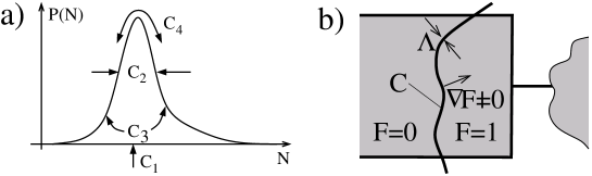
Figure 1.  : Left panel: An example of a probability distribution illustrating the meaning of the different cumulants. The average is given by $C_{1}$, the width by $C_{2}$, the ’skewness’ by $C_{3}$ and the ’sharpness’ is related to the $C_{4}$. Right panel: schematics of an ideal charge counter in a terminal. The number of charges passing the cross section $C$ are counted.

To connect the CGF to accessible field-theoretical quantities we consider the nonlinear response of our electronic circuit to the time-dependent perturbation

$$H_{c}(t)=\frac{\chi}{2e}I_{c}(t)=\mp\frac{\chi}{2e}\int d^{3}x\Psi^{\dagger}({\mathbf{x}},t)\hat{j}_{c}({\mathbf{x}})\Psi({\mathbf{x}},t)\,,$$ (13)

where the $+(-)$ sign is taken on the lower(upper) part of the Keldysh contour. The operator $\hat{j}_{c}({\mathbf{x}})$ is the operator of the current through a cross section $c$, depicted in Fig. 1. We allow here for multi-component field operators, such as spin or Nambu for example. Matrices in this subspace are denoted with a $\hat{}$. Since we are aiming at the total charge counting statistics, we will assume that $\chi$ is nonzero and constant in a finite time interval $[0,t_{0}]$.

The unperturbed system evolves according to a Hamiltonian $H_{0}=\int d^{3}x\Psi^{\dagger}({\mathbf{x}})\hat{h}_{0}({\mathbf{x}})\Psi({\mathbf{x}})$, where $\hat{h}_{0}$ is the usual single-particle Hamiltonian of the system. The equation of motion for the matrix Green’s function subject to $H=H_{0}+H_{c}(t)$ reads (in the Keldysh matrix representation)

$$\left[i\frac{\partial}{\partial t}-\hat{h}_{0}({\mathbf{x}})+\frac{\chi}{2e}\bar{\tau}_{3}\hat{j}_{c}({\mathbf{x}})\right]\check{G}({\mathbf{x}},t;{\mathbf{x}^{\prime}},t^{\prime};\chi)=\delta(t-t^{\prime})\delta({\mathbf{x}}-{\mathbf{x}^{\prime}})\,,$$ (14)

Here $\bar{\tau}_{3}$ denotes the third Pauli matrix in the Keldysh space. The relation of the Green’s function (14) to the CGF (12) is obtained from a diagrammatic expansion in $\chi$. One finds the simple relation (see App. 6.2)

$$\frac{\partial S(\chi)}{\partial\chi}=\frac{it_{0}}{e}I(\chi)\,.$$ (15)

The counting current $I(\chi)$ is obtained from the $\chi$-dependent Green’s function via

$$I(\chi)=\int d^{3}x\left.\textrm{Tr}\left[\bar{\tau}_{3}\hat{j}_{c}({\mathbf{x}})\check{G}({\mathbf{x}},t;{\mathbf{x}^{\prime}},t;\chi)\right]\right|_{{\mathbf{x}}\to{\mathbf{x}^{\prime}}}\,.$$ (16)

Since we are assuming a static situation, the r.h.s. of Eq. (16) is time-independent. The relations (14)-(16) offer a very general way to obtain the full counting statistics of any system. It is, however, difficult to find the Green’s function in the general case.

For a mesoscopic transport problem there is a particularly simple way to access the full counting statistics, based on the separation into terminals (or reservoirs) and an active part, the first providing boundary conditions, and the second being responsible for the resistance. Let us consider the equation of motion for the Green’s function inside a terminal for the following parameterization of the current operator in Eq. (13)

$$\hat{j}_{c}({\mathbf{x}})=(\nabla F({\mathbf{x}}))\lim_{{\mathbf{x}}\to{\mathbf{x}^{\prime}}}\frac{ie}{2m}\left(\nabla_{\mathbf{x}}-\nabla_{{\mathbf{x}}^{\prime}}\right)\hat{\sigma}_{3}\,.$$ (17)

$F({\mathbf{x}})$ is chosen such that it changes from 0 to 1 across a cross section C, which intersects the terminal, but is of arbitrary shape, see Fig. 1. Here we have added a matrix $\hat{\sigma}_{3}$ to the current operator, which accounts for possible multicomponent field operators like in the case of superconductivity. The change from 0 to 1 should occur on a length scale $\Lambda$, for which we assume $\lambda_{F}\ll\Lambda\ll l_{imp},\xi_{0}$ (Fermi wave length $\lambda_{F}$, impurity mean free path $l_{imp}$, and coherence length $\xi_{0}=v_{F}/2\Delta$). Under this assumption we can reduce Eq. (14) to its quasiclassical version (see Ref. [30] and App. 7.1). This is usually a very good approximation, since all currents in a real experiment are measured in normal Fermi-liquid leads.

The Eilenberger equation in the vicinity of the cross section reads

$${\mathbf{v}_{F}}\nabla\check{g}({\mathbf{x}},{\mathbf{v}_{F}},t,t^{\prime},\chi)=\left[-i\frac{\chi}{2}(\nabla F({\mathbf{x}})){\mathbf{v}_{F}}\check{\tau}_{K}\,,\,\check{g}({\mathbf{x}},{\mathbf{v}_{F}},t,t^{\prime},\chi)\right]\,.$$ (18)

Here $\check{\tau}_{K}=\bar{\tau}_{3}\hat{\sigma}_{3}$ is the matrix of the current operator. Other terms can be neglected due to the assumptions we have made for $\Lambda$. The counting field can then be eliminated by the gauge-like transformation

$$\check{g}({\mathbf{x}},{\mathbf{v}_{F}},t,t^{\prime},\chi)=e^{-i\chi F({\mathbf{x}})\check{\tau}_{K}/2}\check{g}({\mathbf{x}},{\mathbf{v}_{F}},t,t^{\prime},0)e^{i\chi F({\mathbf{x}})\check{\tau}_{K}/2}\,.$$ (19)

We assume now that the terminal is a diffusive metal of negligible resistance. Then the Green’s functions are constant in space (except in the vicinity of the cross section C) and isotropic in momentum space. Applying the diffusive approximation [31] in the terminal leads to a transformed terminal Green’s function

$$\check{G}(\chi)=e^{-i\chi\check{\tau}_{K}/2}\check{G}(0)e^{i\chi\check{\tau}_{K}/2}\,,$$ (20)

on the right of the cross section $C$ (where $F({\mathbf{x}}=1$) with respect to the case without counting field. Consequently the counting field is entirely incorporated into a modified boundary condition imposed by the terminal onto the mesoscopic system. Note, that it follows from (17) and (18), that the counting field for a particular terminal vanishes from the equations of motion in the mesoscopic system and the other terminals.

The generalization of this method to the counting statistics for multiterminal structures was performed in [32]. The surprisingly simple result is, that one has to add a separate counting field for each terminal, in which charges are counted. In Sec. 4.1 we demonstrate this for an example, in which an analytic solution can be found. This concludes the derivation of our theoretical method to obtain the FCS.

What are the achievements of this method? We should emphasize that it does not simplify the solution of a specific transport problem, i.e. we still have to know the solution corresponding to the Hamiltonian $H_{0}$. If this solution is not known, the counting field makes this situation not easier. Rather, the method paves a very general way to obtain the FCS, if a method to find the average currents, i.e. for $\chi=0$, is known. In the next section we will introduce such a method, the circuit theory of mesoscopic transport. Initially it was invented to calculate average currents, however the method to obtain the FCS introduced in this section is straightforwardly included.

What is the price to pay? Loosely speaking, the method to obtain the average currents has to be sufficiently general. Usually the absence of a field, which has different signs on the upper and lower part of the Keldysh contour, allows some simplification. For example, in the Keldysh-matrix representation all Green’s functions can be brought into a tri-diagonal form, which is obviously simpler to handle than the full matrix. The method above does not allow this simplification anymore. Or, in other words, the counting rotation (20) destroys the triangular form. Thus, the price we have to pay for an easy determination of the FCS is that we need a method, which respects the full Keldysh-matrix structure in all steps. The circuit theory, which we describe in the next section fulfills this requirement.

2.3 Circuit Theory

A concise formulation of mesoscopic transport is the so-called circuit theory [15, 33]. Its main idea, borrowed from Kirchhoff’s classical circuit theory, is to represent a mesoscopic device by discrete elements. These approximate the layout of an experimental device with arbitrary accuracy, provided one chooses enough elements. In practice one has to find the balance between a small grid size and the computational effort.

We briefly repeat the essentials of the circuit theory. Topologically, one distinguishes three elements: terminals, nodes and connectors. Terminals are the connections to the external measurement circuit and provide boundary conditions, specifying externally applied voltages, currents or phase differences. Besides, they also determine the type of the terminal, i.e. if it is a normal metal or a superconductor. The actual circuit, which is to be studied consists of nodes and connectors, the first determining the approximate layout, and the second describing the connections between different nodes.

The central element of the circuit theory is the arbitrary connector, characterized by a set of transmission coefficients $\{T_{n}\}$. Its transport properties are described by a matrix current found in [33]

$$\check{I}_{12}=-\frac{e^{2}}{\pi}\sum_{n}\frac{2T_{n}\left[\check{G}_{1},\check{G}_{2}\right]}{4+T_{n}\left(\{\check{G}_{1},\check{G}_{2}\}-2\right)}\,.$$ (21)

Here $\check{G}_{1(2)}$ denote the matrix Green’s functions on the left and the right of the contact. We should emphasize that the matrix form of (21) is crucial to obtain the FCS, since it is valid for any matrix structure of the Green’s functions. The electrical current is obtained from the matrix current by

$$I_{12}=\frac{1}{4e}\int dE{\rm Tr}\check{\tau}_{K}\check{I}_{12}\,.$$ (22)

A special case is a diffusive wire of length $L$ in the presence of proximity effect. If $L$ is longer than other characteristic lengths like $\xi_{0}$, decoherence between electrons and holes becomes important and the transmission eigenvalue ensemble is not known. Instead, one solves the diffusion-like equation [31]

$$\nabla D({\mathbf{x}})\check{G}({\mathbf{x}})\nabla\check{G}({\mathbf{x}})=\left[-iE\hat{\tau}_{3},\check{G}({\mathbf{x}})\right]\,.$$ (23)

The matrix current is now given by

$$\check{I}({\mathbf{x}})=-\sigma({\mathbf{x}})\check{G}({\mathbf{x}})\nabla\check{G}({\mathbf{x}})\,.$$ (24)

In these equations, $D({\mathbf{x}})$ the diffusion coefficient and $\sigma({\mathbf{x}})=2e^{2}N_{0}D({\mathbf{x}})$ is the conductivity. In general this equation can only be solved numerically, but in some special cases (e.g. for $E=0$) an analytic solution is possible.

If the circuit consists of more than one connector, the transport properties can be found from the circuit theory by means of the following circuit rules. We take the Green’s functions of the terminals as given and introduce for each internal node an (unknown) Green’s function. The two rules determining the transport properties of the circuit completely are

1. $\check{G}^{2}_{j}=\check{1}$ for the Green’s functions of all internal nodes $j$.

2. The total matrix current in a node is conserved: $\sum_{i}\check{I}_{ij}=0$, where the sum goes over all nodes or terminals connected to node $j$ and each matrix current is given by (21) or (24), depending on the type of the connector.

An important feature of the circuit theory in the form presented above is that it accounts for any matrix structure (i.e. Keldysh, Nambu, Spin, etc.). Thus, we can straightforwardly obtain the FCS along the lines of Sec. 2.2. If the charges in a terminal are counted, we have to apply a counting rotation (20) to the terminal Green’s function. The counting-rotation matrix has the form $\check{\tau}_{K}=\hat{\sigma}_{3}\bar{\tau}_{3}$, where $\hat{\sigma}_{i}(\bar{\tau}_{i})$ denote Pauli-matrices in Nambu(Keldysh)-space. Then we can employ the circuit rules to find the $\chi$-dependent Green’s function and finally obtain the total CGF by integrating all currents into the terminals over their respective counting fields (see [32] and [18] for more details).

3 Two-Terminal Contacts

In this chapter we demonstrate several examples of the FCS of contacts between two terminals, see Fig. 2. One can easily derive a number of rather general results, such as Poisson statistics in the case of tunnel junction, or binomial statistics for single channel contacts of transparency $T$. All these results can be found from a general CGF [16], which depends on the ensemble of transmission eigenvalues $\{T_{n}\}$. To illustrate specific examples, we will compare the cases of transport between two normal terminals or between one superconducting and one normal terminal. In the end, the statistics of an equilibrium supercurrent is discussed.

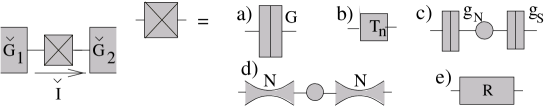
Figure 2.  : Two terminal contacts. The leftmost picture shows a general two-terminal contact. A matrix current $\check{I}$ is flowing between terminals, characterized by Green’s functions $\check{G}_{1,2}$. Several connectors (a-e) are described in the text and depicted as: a) tunnel junction, b) arbitrary connector with transmission eigenvalues $\{T_{n}\}$, c) two tunnel junctions in series with conductances $g_{N}(g_{S})$, respectively, d) a chaotic cavity connected by $N_{ch}$ channels to the leads, and e) a diffusive wire, characterized by a resistance $R_{N}$.

3.1 Tunnel Junction

The counting statistics of a tunnel junction contact can be obtained from a direct expansion of the matrix current (21), if $T_{n}\ll 1$ for all $n$. It coincides with the result obtained by means of the tunneling Hamiltonian [34]. The matrix current takes the form

$$\check{I}_{\rm tun}(\chi)=\frac{G_{T}}{2}\left[\check{G}_{1}(\chi),\check{G}_{2}\right]\,.$$ (25)

Here the matrix current depends only on the tunneling conductance $G_{T}=(e^{2}/\pi)$ $\sum_{n}T_{n}$ of the contact, and we have arbitrarily chosen to count the charges in terminal 1. Now, the counting current is

$$I(\chi)=\frac{G_{T}}{8e}\int dE\textrm{Tr}\left(\check{\tau}_{K}\left[\check{G}_{1}(\chi),\check{G}_{2}\right]\right)\,.$$ (26)

We use the pseudo-unitarity $\check{\tau}_{K}^{2}=\check{1}$ to express the counting rotation as $\exp(i\chi\check{\tau}_{K}/2)=\check{\tau}_{+}\exp(i\chi/2)+\check{\tau}_{-}\exp(-i\chi/2)$, where $\check{\tau}_{\pm}=(1\pm\check{\tau}_{K})/2$. Then the current has the form

$$I(\chi) = \frac{e}{t_{0}}\left[N_{12}e^{-i\chi}-N_{21}e^{i\chi}\right]\,,\,$$ (27)

$$N_{ij} = \frac{t_{0}G_{T}}{4e^{2}}\int dE\textrm{Tr}\left[\check{\tau}_{+}\check{G}_{i}\check{\tau}_{-}\check{G}_{j}\right]\,.$$ (28)

The CGF follows from integrating (27) with respect to $\chi$ and we obtain

$$S(\chi)=-N_{12}(e^{i\chi}-1)-N_{21}(e^{-i\chi}-1)\,.$$ (29)

It is easy to see that the even and odd cumulants obey

$$C_{2n+1}=N_{12}-N_{21}\quad,\quad C_{2n}=N_{12}+N_{21}\,.$$ (30)

If only tunneling processes in one direction occur (say from 1 to 2), $N_{21}=0$ and the average $\bar{N}=N_{12}$. The statistics is Poissonian

$$P_{t_{0}}(N)=e^{-\bar{N}}\frac{\bar{N}^{N}}{N!}$$ (31)

In particular, for the current noise we find the Schottky result $S_{I}=2eI$.

We conclude that the charge counting statistics of a tunnel junction (or more precisely, if the transfer events are rare) is of a generalized Poisson type [34]. If only tunneling events in one directions are possible, the statistics is Poissonian.

3.2 Quantum Contact – General Connector

We consider now a quantum contact characterized by a set of transmission eigenvalues $\{T_{n}\}$. It turns out that the CGF can be obtained in a quite general form, valid for arbitrary junctions between superconductors and/or normal metals.

The matrix current through a quantum contact is described by Eq. (21) and the CGF can then be found from the relation $\partial S(\chi)/\partial\chi=(-it_{0}/4e^{2})$ $\int dE$ ${\rm{Tr}}[\check{\tau}_{\rm K}\check{I}(\chi)]$. Using that $[\check{A},\{\check{A},\check{G}_{2}\}]=0$ for all matrices with $\check{A}^{2}=\check{1}$ the following identity holds

$$\mbox{Tr}\frac{\partial}{\partial\chi}\left\{\check{G}_{1}(\chi),\check{G}_{2}\right\}^{n}=\frac{i}{2}\mbox{Tr}\check{\tau}_{K}\left[\check{G}_{1}(\chi),\check{G}_{2}\right]\left\{\check{G}_{1}(\chi),\check{G}_{2}\right\}^{n-1}\,.$$ (32)

We can therefore integrate (22) with respect to $\chi$ and obtain [16]

$$S(\chi)=-\frac{t_{0}}{2\pi}\sum_{n}\int dE{\textrm{Tr}}\ln\left[1+\frac{T_{n}}{4}\left(\{\check{G}_{1}(\chi),\check{G}_{2}\}-2\right)\right]\;.$$ (33)

This is a very important result. It shows that the counting statistics of a large class of constrictions can be cast in a common form, independent of the contact types. Another important property of Eq. (33) is, that the CGF’s of all constrictions are linear statistics of the transmission eigenvalue distribution, and can therefore be averaged over by standard means (see e.g. [35]). Examples are given in the following sections. Note also, that an expansion of Eq. (33) for $T_{n}\ll 1$ yields the result (29) of the tunnel case.

We will now discuss several illustrative examples. Consider first two normal reservoirs with occupation factors $f_{1(2)}=[\exp((E-\mu_{1(2)})/T_{e})+1]^{-1}$ ($T_{e}$ is the temperature). We obtain the result [12, 13]

$$S(\chi)=-\frac{t_{0}}{\pi}\sum_{n}\int dE\ln\left[1+B_{1n}(E)\left(e^{i\chi}-1\right)+B_{-1n}(E)\left(e^{-i\chi}-1\right)\right]\,.$$ (34)

Here we introduced the probabilities $B_{1n}=T_{n}f_{1}(E)\left(1-f_{2}(E)\right)$ for a tunneling event from 1 to 2 and $B_{-1n}$ for the reverse process. The terms with counting factors $e^{\pm i\chi}-1$ obviously correspond to charge transfers from 1 to 2 (2 to 1). At zero temperature and $\mu_{1}-\mu_{2}=eV\geq 0$ the integration can easily be evaluated and we obtain

$$S(\chi)=-\frac{et_{0}|V|}{\pi}\sum_{n}\ln\left[1+T_{n}\left(e^{i\chi}-1\right)\right]\,.$$ (35)

The corresponding statistics for a single channel with transparency $T$ is binomial

$$P_{t_{0}}(N)={M\choose N}T^{N}(1-T)^{M-N}\,.$$ (36)

Here we have introduced the number of attempts $M=et_{0}V/\pi$, which is the maximal number of electrons that can be sent through one (spin-degenerate) channel in a time interval $t_{0}$ due to the exclusion principle for Fermions.

The FCS of an superconductor-normal metal-contact also follows from Eq. (33) (for a definition of the various Green’s functions see App. 7.4). Evaluating the trace in Eq. (33) the CGF can be expressed as [36]

$$S(\chi)=-\frac{t_{0}}{2\pi}\sum_{n}\int dE\ln\left[1+\sum\limits_{q=-2}^{2}A_{nq}(E)\left(e^{iq\chi}-1\right)\right]\,.$$ (37)

The coefficients $A_{nq}(E)$ are related to a charge transfer of $q\times e$. For example a term $\exp(2i\chi)-1$ corresponds just to an Andreev reflection process, in which two charges are transfered simultaneously [37]. Explicit expressions for the various coefficients are given in Appendix 8.1. For the BCS case, they reproduce the results of Ref. [36]. In the fully gapped single-channel case at energies $k_{B}T_{e}\ll eV\ll\Delta$ only terms corresponding to Andreev reflection ($A_{2}$) are nonzero and the CGF becomes

$$S(\chi)=-\frac{et_{0}|V|}{\pi}\ln\left[1+R_{A}\left(e^{i2\chi}-1\right)\right]\,,$$ (38)

where $R_{A}=T^{2}/(2-T)^{2}$ is the probability of Andreev reflection. The CGF is now $\pi$-periodic, which means that only even numbers of charges are transfered, a consequence of Andreev reflection. The corresponding statistics is binomial

$$P_{t_{0}}(2N)={M\choose N}R_{A}^{N}\left(1-R_{A}\right)^{M-N}\,,\,P_{t_{0}}(2N+1)=0\,.$$ (39)

The number of attempts $M$ is, however, the same as in the normal state.

It is interesting to see how the CGF for normal transport, i. e., Eq. (34), emerges from Eq. (37). Putting $f_{R,A}=0$ and $g_{R,A}=\pm 1$ the coefficients in Eq. (37) can be written as

$$A_{\pm 1} = B_{\pm 1}^{+}+B_{\pm 1}^{-}-2B_{\pm 1}^{+}B_{\pm 1}^{-}-B_{\pm 1}^{+}B_{\mp 1}^{-}-B_{\pm 1}^{-}B_{\mp 1}^{+}\,,$$

$$A_{\pm 2} = B_{\pm 1}^{+}B_{\pm 1}^{-}\;\;;\;\;B_{1}^{\pm}=TB_{1}(\pm E)\,,B_{-1}^{\pm}=TB_{-1}(\pm E)\,,$$

The argument of the ’ln’ in Eq. (37) factorizes in positive and negative energy contributions

$$\ln\left[1+\sum\limits_{q=-2}^{2}A_{q}\left(e^{iq\chi}-1\right)\right]=\sum\limits_{s=\pm}\ln\left[1+\sum\limits_{q=-1}^{1}B_{q}^{s}\left(e^{iq\chi}-1\right)\right]\,.$$ (40)

Integrating over energy both terms give the same contribution, and the CGF results in Eq. (34). This shows explicitly how the positive and negative energy quasiparticles are correlated in the Andreev reflection process.

3.3 Double Tunnel Junction

We now consider a diffusive island (or a chaotic cavity) connected to two terminals by tunnel junctions with respective conductance $g_{1}$ and $g_{2}$ [18]. We assume for the conductance of the island $g_{island}\gg g_{1,2}\gg e^{2}/h$, so we can neglect charging effects. This provides a simple application of the circuit theory. The layout is shown in Fig. 2c. The central node is described by an unknown Green’s function $\check{G}_{c}$. We have two matrix currents entering the node, which obey a conservation law:

$$0=\check{I}_{1}+\check{I}_{2}=\frac{1}{2}\left[g_{1}\check{G}_{1}+g_{2}\check{G}_{2},\check{G}_{c}\right]\,.$$ (41)

Using the normalization condition $\check{G}_{c}^{2}=1$ the solution is

$$\check{G}_{c}=\frac{g_{1}\check{G}_{1}+g_{2}\check{G}_{2}}{\sqrt{g_{1}^{2}+g_{2}^{2}+g_{1}g_{2}\left\{\check{G}_{1},\check{G}_{2}\right\}}}\,.$$ (42)

We can integrate the current $I(\chi)\sim\rm{Tr}\check{\tau}_{K}\check{I}_{1}$ and obtain the CGF

$$S(\chi)=-\frac{t_{0}}{4e^{2}}\int dE{\rm Tr}\sqrt{g_{1}^{2}+g_{2}^{2}+g_{1}g_{2}\left\{\check{G}_{1},\check{G}_{2}\right\}}\;.$$ (43)

Again, this result is valid for all types of contacts between normal metals and superconductors.

We first evaluate the trace for two normal leads and find

$$S(\chi)=-\frac{t_{0}}{2e}\int dE\times$$

$$\sqrt{(g_{1}+g_{2})^{2}+4g_{1}g_{2}\left(f_{1}(1-f_{2})(e^{i\chi}-1)+f_{2}(1-f_{1})(e^{-i\chi}-1\right))}\,.$$

We observe that the CGF contains again counting factors corresponding to charge transfer from 1 to 2 and vice versa. In contrast to the Poissonian case for a tunnel junction, Eq. (29), the charge transfers are not independent, but correlated by the square-root function. At zero temperature and $\mu_{1}-\mu_{2}=eV>0$ we find the result,

$$S(\chi)=-\frac{t_{0}V}{2e}\sqrt{(g_{1}+g_{2})^{2}+4g_{1}g_{2}(e^{i\chi}-1)}\,.$$ (45)

There are two relatively simple limits. If the two conductances are very different (e.g. $g_{1}\ll g_{2}$), we return to Poissonian statistics:

$$S(\chi)=-\frac{t_{0}Vg_{1}}{e}(e^{i\chi}-1)\,.$$ (46)

On the other hand, in the symmetric case $g_{1}=g_{2}=g$ we find [38]

$$S(\chi)=-\frac{t_{0}Vg}{e}(e^{i\chi/2}-1)\,,$$ (47)

and the cumulants are

$$C_{n}=\frac{\bar{N}}{2^{n-1}}\quad,\quad\bar{N}=\frac{t_{0}g|V|}{2e}\,.$$ (48)

The suppression factor $1/2$, which occurs already in the Fano factor, carries forward to all cumulants. Note, that the same kind of statistics (3.3) follows also from a Master equation [38, 39].

The CGF (43) for the transport between a normal metal and a superconductor (at zero temperature, for simplicity) reads [18]

$$S(\chi)=-\frac{t_{0}V}{e\sqrt{2}}\sqrt{g_{1}^{2}+g_{2}^{2}+\sqrt{\left(g_{1}^{2}+g_{2}^{2}\right)^{2}+4g_{1}^{2}g_{2}^{2}(e^{i2\chi}-1)}}\,.$$ (49)

Thus, the influence of the superconductor is two-fold: charges are transfered in units of $2e$ (indicated by the $\pi$-periodicity) and another square root is involved in the CGF, resulting from the higher order correlations. In the limit that both conductances are very different (e.g. $g_{1}\ll g_{2}$) we obtain again Poissonian statistics

$$S(\chi)=-\frac{t_{0}V}{e}\frac{g_{1}^{2}}{g_{2}}\left(e^{i2\chi}-1\right)\,.$$ (50)

This corresponds to uncorrelated transfers of pairs of charges. Consequently we obtain for the cumulants

$$C_{n}=2^{n-1}\bar{N}\quad,\quad\bar{N}=\frac{2t_{0}Vg_{1}^{2}}{eg_{2}}\,,$$ (51)

and the effective charge $2e$ can indeed be found from the Fano factor. The transport properties at finite energies and magnetic fields of this structure have recently been addressed in [19] and [20].

3.4 Symmetric Chaotic Cavity

Another interesting system is the chaotic cavity, i. e. a small island coupled to terminals by perfectly transmitting contacts (with $N_{ch}\gg 1$ channels). This system is described by the circuit depicted in Fig. 2d. The matrix current between terminal 1 and the cavity is $\check{I}_{1}=N_{ch}(e^{2}/\pi)[\check{G}_{1},\check{G}_{c}]/(2+\{\check{G}_{1},\check{G}_{c}\})$. Similar as in the previous chapter, the current conservation reads now

$$0=\frac{\left[\check{G}_{1},\check{G}_{c}\right]}{2+\left\{\check{G}_{1},\check{G}_{c}\right\}}+\frac{\left[\check{G}_{2},\check{G}_{c}\right]}{2+\left\{\check{G}_{2},\check{G}_{c}\right\}}\,,$$ (52)

which is solved by the solution (42) for $g_{1}=g_{2}$. The integration of (22) leads to

$$S(\chi)=-N_{ch}\frac{t_{0}}{2\pi}\int dE\textrm{Tr}\ln\left[2+\sqrt{2+\left\{\check{G}_{1}(\chi)\,,\,\check{G}_{2}\right\}}\right]\,.$$ (53)

The interpretation of this result is straightforward. As we have seen in Sec. 3.2, the $\ln$ appeared already in the FCS of a quantum point contact (leading to binomial statistics). The square-root we encountered already in the previous section and we attribute it to inter-mode mixing on the central node (’cavity noise’).

For normal leads at zero temperature and applied bias voltage $V$ we obtain (with the number of attempts $M=N_{ch}t_{0}eV/\pi$)

$$S(\chi)=-2M\ln\left[1+e^{i\chi/2}\right]\,.$$ (54)

On the other hand, in the case of Andreev reflection we find

$$S(\chi)=-2M\ln\left[2+e^{i[\chi{\rm mod}\pi]}+2\sqrt{1+e^{i[\chi{\rm mod}\pi]}}\right]\,,$$ (55)

where the $\pi$-periodicity reflects the fact that charges are transfered in pairs.

3.5 Diffusive Connector

A metallic strip of length $L$ with purely elastic scattering, characterized by an elastic mean free path $l$, is called a diffusive connector if $l\ll L$. Its transport properties are governed by the diffusion-like Usadel equation, Eq. (23). In the case of proximity transport the r.h.s. of Eq. (23) accounts for decoherence of electrons and hole during their diffusive motion along the normal wire. This term has the form of a leakage current, if the l.h.s. is considered as a conservation law for the matrix current [33]. Note that the electric current is still conserved, it is only loss of coherence which occurs. In general the solution of the full equation is rather complicated and can only be found numerically for the full parameter range. There is, however, one case, in which an analytic solution is possible, namely if the r.h.s. of Eq. (23) vanishes. This is either the case for purely normal transport, when electrons and holes are transported independently, or for $E=0$, which means we are restricted to low temperatures and voltages. The scale here is set by the Thouless energy $E_{Th}$ (given by $\hbar D/L^{2}$ for a wire of uniform cross section). At this scale the famous reentrance effect of the conductance occurs [40]. This regime was studied in Ref. [17] and will be discussed in connection with experimental results for the current noise in the article by Reulet et al. in this book. Numerical results for equilibrium counting statistics in the full parameter range are discussed below.

We now concentrate on the analytic solution in a quasi-one-dimensional geometry, i. e. we assume a wire of uniform cross section connects two reservoirs located at $x=0$ and $x=L$. It is characterized by a conductivity $\sigma(x)$, which in general could depend on $x$, e. g. due to an inhomogeneous concentration of scattering centers. The diffusion equation is then indeed a conservation law for the matrix current density

$$\frac{\partial}{\partial x}\check{j}=0\quad,\quad\check{j}=-\sigma(x)\check{G}(x)\frac{\partial}{\partial x}\check{G}(x)\,.$$ (56)

This equation has to be solved with the boundary condition that $\check{G}(0)=\check{G}_{1}$ and $\check{G}(L)=\check{G}_{2}$. It follows from Eq. (56) and the normalization condition $\check{G}^{2}(x)=\check{1}$ that $\check{G}(x)$ obeys the equation

$$\check{j}={\textrm{const.}}\quad,\quad\frac{\partial}{\partial x}\check{G}(x)=-\frac{1}{\sigma(x)}\check{G}(x)\check{j}\,.$$ (57)

This is an homogeneous first-order differential equation, which is easily solved. Using the boundary conditions we find the solution

$$\check{G}(L)=\check{G}(0)e^{\check{I}/g_{d}}\;,\;g_{d}=\frac{A}{\int_{0}^{L}dx/\sigma(x)}\,,$$ (58)

where $g_{d}$ is the conductance of the wire and $A$ its cross section. The current is thus given by [14]

$$\check{I}(\chi)=-g_{d}\ln\left(\check{G}_{1}(\chi)\check{G}_{2}\right)\,,$$ (59)

where we have reinserted the dependence on the counting field $\chi$. To find the CGF we have to find the integral $\int d\chi$Tr$\check{\tau}_{K}\check{I}(\chi)$ with respect to the counting field. Expanding the $\ln$ and using repeatedly the normalization condition the results is

$$S(\chi)=-\frac{t_{0}g_{d}}{8e^{2}}\int dE\textrm{Tr}\left[\textrm{acosh}^{2}\left(\frac{1}{2}\left\{\check{G}_{1}(\chi),\check{G}_{2}\right\}\right)\right]\,.$$ (60)

This is the counting statistics for a general diffusive contact (under the restrictions mentioned above). The first thing to note is that from the properties of the wire only the conductance enters and this holds for all cumulants. In this sense Eq. (60) shows that the entire FCS is universal. In our derivation, we have assumed a wire of uniform cross section, but it has been shown [9] that this also holds for an arbitrary shape of the wire (as long as it can be considered as quasi one-dimensional). We should also mention, that one could have obtained the same result, by averaging the CGF (12) over the bimodal distribution of transmission eigenvalues [41, 9].

Now we evaluate the trace in Eq. (60) for normal metals at zero temperature and applied bias voltage $eV$. We obtain

$$S(\chi)=-\frac{t_{0}g_{d}V}{4e}\textrm{acosh}^{2}\left(2e^{i\chi}-1\right)\,,$$ (61)

which coincides with the results of Refs. [14, 42].

In the case of Andreev transport the easiest way to obtain the CGF is as follows. We have already previously noted, that Eq. (61) follows from averaging Eq. (35) with the transmission eigenvalue distribution $\rho(T)=(2e^{2}/g_{d}\pi)/T\sqrt{1-T}$ for a diffusive metal [9, 41]. Now, the CGF for Andreev transport Eq. (38) has the same form as in the case of normal transport, provided we replace $\chi$ with $2\chi$ and the transmission eigenvalue $T_{n}$ with the Andreev reflection probability $R_{A}(T_{n})$. A simple calculation shows, that the $R_{A}$ are distributed according to the same distribution as the normal transmission eigenvalues (up to a factor of 1/2). Thus, we can immediatly read off the CGF for the diffusive SN-wire in the limit of zero temperature and $eV\ll E_{Th}$ from Eq. (61) and obtain

$$S(\chi)=-\frac{t_{0}g_{d}V}{8e}\textrm{acosh}^{2}\left(2e^{2i\chi}-1\right)\,.$$ (62)

As a consequence the relation between the cumulants in the SN-case, $C_{n}^{\rm SN}$, and the normal case, $C_{n}^{\rm NN}$, is

$$C_{n}^{\rm SN}=2^{n-1}C_{n}^{\rm NN}\,.$$ (63)

We observe that we can read off the effective charge from the ratio $C_{n}^{\rm SN}/C_{n}^{\rm NN}$ $=$ $(q_{eff}/e)^{n-1}$ and, indeed, find $q_{eff}=2e$. We should emphasize, however, that this is a special property of the diffusive connector. Our prove of Eq. (63) is valid as long as $eV\ll E_{Th}$, and it is not clear, wether Eq. (63) is true also for $eV\gg E_{Th}$

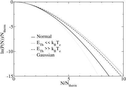
Figure 3.  : Equilibrium distribution of the current fluctuations in a diffusive SN-contact. We observe a) a strong deviation of all distributions from a Gaussian b) enhanced fluctuations in the superconducting case, and c) differences between proximity effect and coherent transport. Note, that the second cumulant (i.e. the thermal noise) is the same for all displayed curves.

The counting statistics in equilibrium for arbitrary temperature $T_{e}$ was studied in Ref. [17]. By a numerical solution of Eq. (23), it is possible to evaluate the integral over $\chi$ in the inversion of Eq. (4) in the saddle point approximation, i.e. we take $\chi$ as complex and expand the exponent around the complex saddle point $\chi=ix_{0}$. The integral yields then $P(N)\approx\exp(-S(ix_{0})-x_{0}N)$, which we plot implicitly as a function of $N(x_{0})=\partial S(ix_{0})/\partial x_{0}$. Results of this calculation are displayed in Fig. 3. The charge number N is normalized by $N_{\rm therm}=g_{d}t_{0}k_{B}T_{e}/e^{2}$. Note that the conductance (and due to the fluctuation-dissipation theorem the noise) is the same in all cases. The solid line shows the distribution in the normal state, which does not depend on the Thouless energy. In our units, this curve is consequently independent on temperature. In the superconducting state the Thouless energy does matter, and the distribution depends on the ratio $E_{\rm Th}/k_{B}T_{e}$. We observe that large fluctuations of the current in the superconducting case are enhanced in comparison to the normal case, and in both cases are enhanced in comparison to Gaussian noise $\sim\exp(-N^{2}/4N_{\rm them})$. The differences between the normal and the superconducting state occur in the regime of non-Gaussian fluctuations.

3.6 Supercurrent

The CGF of a quantum contact, i. e. Eq. (12), can be used to find the counting statistics for a supercurrent between two superconductors at a fixed phase difference $\phi$. This has been done in Ref. [16]. The result can be represented in a form similar to the CGF of the SN-contact (37)

$$S(\chi,\phi)=-\frac{t_{0}}{2\pi}\sum_{n}\int dE\ln\left[1+\sum\limits_{q=-2}^{2}\frac{A_{n,q}^{S}(E,\phi)}{Q_{n}(E,\phi)}\left(e^{iq\chi}-1\right)\right]\,.$$ (64)

Explicit expressions for the coefficients are given in Appendix 8.2. To find the statistics of the charge transfer, we will treat two separate cases.

Gapped superconductors. If the two leads are gapped like BCS superconductors, the spectral functions are given by Eq. (119). Here we account for a finite lifetime $\delta$ of the Andreev bound states, e. g. due to phonon scattering. The supercurrent in a one-channel contact of transparency $T_{1}$ is solely carried by Andreev bound states with energies $\pm\Delta(1-T_{1}\sin^{2}\phi/2)^{1/2}\equiv\pm E_{B}(\phi)$. The importance of these bound states can be seen from the coefficient $Q(E,\phi)$ (see Eq. (130)), which may become zero and will thus produce singularities in the CGF. The broadening $\delta$ shifts the singularities of $Q(E,\phi)$ into the complex plane and allows an expansion of the coefficients $A_{1,q}^{S}$ close to the bound state energy. Performing the energy integration the CGF results in

$$S(\chi,\phi)=-2t_{0}\delta\sqrt{1-\chi^{2}\frac{I_{1}^{2}(\phi)}{4\delta^{2}}-i\chi\frac{I_{1}(\phi)}{\delta}\tanh\left(\frac{E_{B}(\phi)}{2k_{B}T_{e}}\right)}\,,$$ (65)

where $I_{1}(\phi)=\Delta^{2}T_{1}\sin(\phi)/2E_{B}(\phi)$ is the supercurrent carried by one bound state. In deriving (65) we have also assumed that $\chi\ll 1$. This corresponds to a restriction to “long trains” of electrons transfered, and the discreteness of the electron transfer plays no role here. Fast switching events become less probable at low temperatures and are neglected here. In the saddle point approximation and for $\gamma(\phi)\equiv 1/\cosh(E_{B}(\phi)/2T_{e})\ll 1$ the FCS can be found. We express the transfered charge in terms of the current normalized to the zero temperature supercurrent: $j(\phi)=eN/t_{0}I_{1}(\phi)$. We find for the current distribution in the saddle point approximation

$$P(j,\phi)\sim\frac{1}{\gamma}\exp\left[2\delta t_{0}\left(\gamma(\phi)\sqrt{1-j^{2}(\phi)}-j(\phi)\sqrt{1-\gamma^{2}(\phi)}\right)\right])\,,$$ (66)

for $|j(\phi)|\leq 1$ and zero otherwise. At zero temperature Eq. (66) approaches $P(j,\phi)\to\delta(j-1)$. Thus the charge transfer is noiseless. At finite temperature, on the other hand, the distribution (66) confirms the picture of switching between Andreev states which carry currents in opposite directions, suggested in Ref. [43]. The previous result is valid under the following conditions. In the energy integration it was assumed that the bound states are well defined. For small transmission the distance of the bound state to the gap edge is $\approx T_{1}\Delta$. Thus, to have well-defined bound states we have to require $\delta<T_{1}\Delta$. Similarly, for a highly transmissive contact and a small phase difference we require $\phi\sim eN/t_{0}I_{\rm c}>\delta/\Delta$. The statistics beyond these limits is similar to what is discussed in the following.

Tunnel junction/gapless superconductors. Let us now consider the supercurrent statistics between two weak superconductors, where the Green’s functions can be expanded in $\Delta$ for all energies. One can see that this is equivalent to the tunnel result (29). It has the form

$$S(\chi,\phi)=-N_{+}(\phi)(e^{i\chi}-1)-N_{-}(\phi)(e^{-i\chi}-1)\,.$$ (67)

where

$$N_{\pm}(\phi)=\frac{t_{0}}{2}\left(P_{\rm s}(\phi)\pm I_{\rm s}(\phi)\right)\,.$$ (68)

This form of the CGF shows that the FCS is expressed in terms of supercurrent $I_{\rm s}(\phi)$ and noise $P_{\rm s}(\phi)$ only. Supercurrent and current noise are

$$I_{\rm s}(\phi)=-\frac{G_{T}}{4}\textrm{Re}\int dE\textrm{Tr}\left\{\hat{\sigma}_{3}\left[\hat{R}_{1}(E,\phi),\hat{R}_{2}(E)\right]\right\}\tanh\left(\frac{E}{2k_{B}T_{e}}\right)\,,$$ (69)

$$P_{\rm s}(\phi)=-\frac{G_{T}}{4}\textrm{Re}\int dE\textrm{Tr}\left\{\hat{\sigma}_{3}\hat{A}_{1}(E,\phi)\hat{\sigma}_{3}\hat{R}_{2}(E)\right\}\frac{1}{\cosh^{2}\left(\frac{E}{2k_{B}T_{e}}\right)}\,.$$ (70)

Here $G_{T}$ is the normal-state conductance of the contact. Eq. (70) shows that $P_{\rm s}$ vanishes at zero temperature, whereas $I_{\rm s}$ vanishes at $T_{\rm c}$. Therefore, there is some crossover temperature below which $P_{\rm s}<|I_{\rm s}|$. In this limit one of the coefficients $N_{\pm}$ becomes negative and the interpretation, that the CGF (67) corresponds to a generalized Poisson distribution, makes no sense anymore. In fact, the CGF leads to ’negative probabilities’ and does not correspond to any probability distribution, The origin of this failure is the broken U(1)-symmetry the superconducting state. Nevertheless the FCS can be used to predict the outcome of any charge transfer measurement, as is discussed in detail in Refs. [16, 28, 44].

4 Multi-Terminal Structures

Many mesoscopic transport experiments are performed in multi-terminal configurations. An example is shown in Fig. 4. Due to the quantum nature of the charge carriers, interesting non-local effects can appear, such as sensitivity of measured voltage differences to changes in the setup outside the current path. Obviously, the same is true for current fluctuations and for the full counting statistics. These are sensitive to the quantum correlations between the charge carriers, which can have a nonlocal character. In terms of counting statistics this means, for example, that the joint probability to count $N_{1}$ particles in terminal 1 and $N_{2}$ particles in terminal 2 can not be factorized into separate probabilities for the two events.

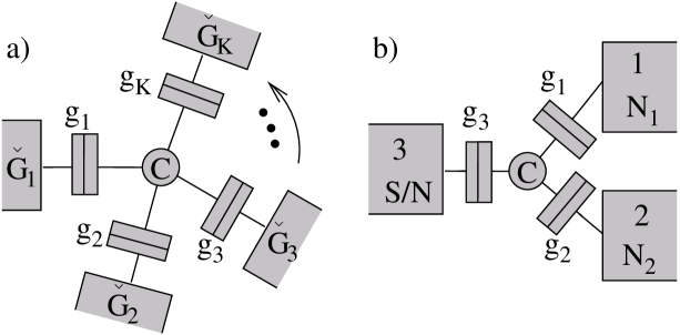
Figure 4.  : a) An example for a multi-terminal structure. $K$ terminals are connected to a central node by tunnel junctions b) Three-terminal structure. Two different voltage configurations are considered. In the first case, all terminals are normal metals. A bias voltage is applied between terminal 1 and terminal 2, whereas terminal 3 is operated as a voltage probe (no mean current). In the second case we consider a beam splitter configuration. A supercurrent or normal current in terminal 3 is divided in (or merged from) two normal currents from terminals 1 and 2. Here, we assume that the same potential is applied to terminals 1 and 2.

4.1 General Result for Multi-Tunnel Geometry

The generalization of the method, introduced in Section 2 for two terminals, to many terminals is straightforward [32]. The counting field $\chi$ is replaced by a vector $\vec{\chi}$, with dimension equal to the number of terminals. For brevity we collect the charges passing each terminal into a vector $\vec{N}$. The current in each terminal is coupled to the respective component of the counting field by an expression like (13). Following the procedure outlined in Sections 2.2 and 2.3 the result is, that the Green’s function of each terminal acquires its own counting field $\chi_{n}$. The rules, that determine the transport properties, remain essentially unchanged.

The procedure outlined above is best illustrated by an example. We consider a node connected to $K$ terminals via tunnel junctions with conductances $g_{k}$. This setup is shown in Fig. 4a. Each terminal is described by a Green’s function $\check{G}_{k}(\chi_{k})$ ($k=1..K$), which is related to the terminal’s usual Green’s function by a counting rotation (20). We do not need to specify yet, whether the terminals are superconducting or normal. The goal is to find (for arbitrary applied voltages and temperatures) the joint probability $P_{t_{0}}(N_{1},N_{2},...,N_{K})$, that $N_{1}$ particles enter through terminal 1, $N_{2}$ particles through terminal 2, …, and $N_{K}$ particles through terminal $K$. Correspondingly we define the cumulant generating function

$$e^{-S(\vec{\chi})}=\sum_{N_{1},N_{2},\cdots,N_{K}}P_{t_{0}}(\vec{N})e^{i\vec{N}\vec{\chi}}\,.$$ (71)

The central node is described by a Green’s function $\check{G}_{c}(\vec{\chi})$, which has to be determined from the circuit rules. The matrix currents through terminal $k$ is given by $\check{I}_{k}=-(g_{k}/2)[\check{G}_{k}(\chi_{k}),\check{G}_{c}(\vec{\chi})]$ and current conservation on the node can be written as

$$0=\sum_{k=1}^{K}\check{I}_{k}=\frac{1}{2}\left[\sum_{k=1}^{K}g_{k}\check{G}_{k}(\chi_{k}),\check{G}_{c}(\vec{\chi})\right]\,.$$ (72)

This equation (together with the normalization condition $\check{G}_{c}^{2}(\vec{\chi})=\check{1}$) is solved by

$$\check{G}_{c}(\vec{\chi})=\frac{\sum_{k=1}^{K}g_{k}\check{G}_{k}(\chi_{k})}{\sqrt{\sum_{k,l=1}^{K}g_{k}g_{l}\left\{\check{G}_{k}(\chi_{k}),\check{G}_{l}(\chi_{l})\right\}}}\,.$$ (73)

The CGF is found from integrating the relations $\partial S(\vec{\chi})/\partial\chi_{k}=(-it_{0}/e)$ $I_{k}(\vec{\chi})$, where $I_{k}(\vec{\chi})=(1/4e)\int dE$Tr$\check{\tau}_{K}\check{I}_{k}(\vec{\chi})$. The CGF is then determined up to an additive constant, which is fixed by the normalization $S(\vec{0})=0$ and neglected in the following. The result is [18]

$$S(\vec{\chi})=-\frac{t_{0}}{4e^{2}}\int dE\;\textrm{Tr}\sqrt{\sum\nolimits_{k,l=1}^{K}g_{k}g_{l}\left\{\check{G}_{k}(\chi_{k}),\check{G}_{l}(\chi_{l})\right\}}\,.$$ (74)

This provides the counting statistics for an arbitrary multi-terminal structure of the type shown in Fig. 4. Below we discuss several examples.

4.2 Normal Metal Multi-Terminal Structures

In the case that all terminals are normal metals, we can evaluate Eq. (74) further. All terms under the square root are proportional to the unit matrix and the trace can be taken easily with the result [45]

$$S(\vec{\chi}) = -\frac{t_{0}g_{\Sigma}}{2e^{2}}\int dE\times$$

$$\sqrt{1+\sum\nolimits_{k,l=1}^{K}t_{kl}\left[f_{k}(1-f_{l})e^{i(\chi_{k}-\chi_{l})}+f_{l}(1-f_{k})e^{i(\chi_{l}-\chi_{k})}\right]}\,,$$

where $g_{\Sigma}=\sum_{k=1}^{K}g_{k}$ and $t_{kl}=2g_{k}g_{l}/g_{\Sigma}^{2}$. The argument of the square root is the sum over all tunneling events from between the terminals. For two terminals we recover the result (3.3).

Let us now consider three normal-metal terminals, one of which is operated as voltage probe, i.e. no average current enters the terminal. This layout is depicted in Fig. 4. We assume for the applied potentials that $V_{1}<V_{3}<V_{2}$. Terminal 3 is operated as a voltage probe and it follows, that $V_{3}=(g_{1}V_{1}+g_{2}V_{2})/(g_{1}+g_{2})$. At zero temperature the energy integration yields

$$S(\vec{\chi}) = -\frac{t_{0}g_{\Sigma}V}{2e}\left[\frac{g_{2}}{g_{1}+g_{2}}\sqrt{1+t_{13}(e^{i(\chi_{3}-\chi_{1})}-1)+t_{12}(e^{i(\chi_{2}-\chi_{1})}-1)}\right.$$ (76)

$$\left.+\frac{g_{1}}{g_{1}+g_{2}}\sqrt{1+t_{23}(e^{i(\chi_{2}-\chi_{3})}-1)+t_{12}(e^{i(\chi_{2}-\chi_{1})}-1)}\right]\,.$$

The CGF separates into two terms. The first term corresponds to the energy window $eV_{3}>E>eV_{1}$, in which transport is only possible between terminals 1 and 3 or between 1 and 2. The second term results from the energy window $eV_{2}>E>eV_{3}$, in which no electrons can enter into terminal 2.

We now consider a different configuration: an instreaming current is divided into two outgoing currents. This corresponds to the voltage configuration $V=V_{1}=V_{2}>V_{3}=0$. The corresponding CGF is

$$S(\vec{\chi})=-\frac{t_{0}g_{\Sigma}V}{2e}\sqrt{1+t_{13}(e^{i(\chi_{1}-\chi_{3})}-1)+t_{23}(e^{i(\chi_{2}-\chi_{3})}-1)}\,.$$ (77)

In the limit $g_{2},g_{1}\gg g_{3}$ or vice versa the CGF takes the form

$$S(\vec{\chi})=-\frac{t_{0}g_{\Sigma}V}{4e}\left(t_{13}(e^{i(\chi_{1}-\chi_{3})}-1)+t_{23}(e^{i(\chi_{2}-\chi_{3})}-1)\right)\,,$$ (78)

and the corresponding counting statistics is

$$P(N_{1},N_{2})=e^{-(\bar{N}_{1}+\bar{N}_{2})}\frac{{\bar{N}_{1}}^{N_{1}}}{N_{1}!}\frac{{\bar{N}_{2}}^{N_{2}}}{N_{2}!}\,.$$ (79)

Here $\bar{N}_{i}=(t_{0}V/e)g_{i}g_{3}/4g_{\Sigma}^{2}$. The statistics is a product of two Poisson distributions, i. e. the two transport processes are uncorrelated.

4.3 Superconducting Multi-Terminal Structures

Let us now consider the beam splitter configuration, if the incoming current originates from a superconductor. Here, we have to use the Nambu$\times$Keldysh matrix structure. The layout is as shown in Fig. 4. We choose terminal 3 as superconducting terminal with $V_{3}=0$ and the potential in the two normal terminal is assumed to be the same, $V_{1}=V_{2}=V$. We consider the limit $T\ll eV\ll E_{Th},\Delta$. Transport occurs then only via Andreev reflection, since no quasiparticles in the superconductor are present. The Green’s functions for the terminals can be found in Appendix 7.4. We note, that the pair breaking effect due to a magnetic field in a chaotic dot with the same terminal configuration was studied by Samuelsson and Büttiker [19].

We now evaluate Eq. (74) for the three-terminal setup. The CGF depends only on the differences $\chi_{1}-\chi_{3}$ and $\chi_{2}-\chi_{3}$, which is a consequence of charge conservation and allows to drop the explicit dependence on $\chi_{3}$ below. Introducing $p_{i}=2g_{3}g_{i}/(g_{3}^{2}+(g_{1}+g_{2})^{2})$ we find

$$S(\chi_{1},\chi_{2})=-\frac{Vt_{0}\sqrt{g_{3}^{2}+(g_{1}+g_{2})^{2}}}{\sqrt{2}e}\times$$

$$\sqrt{1+\sqrt{1+p_{1}^{2}(e^{i2\chi_{1}}-1)+p_{2}^{2}(e^{i2\chi_{2}}-1)+2p_{1}p_{2}(e^{i(\chi_{1}+\chi_{2})}-1)}}\,.$$

The inner argument contains counting factors for the different possible processes. A term $\exp(i(\chi_{k}+\chi_{l})-1)$ corresponds to an event in which two charges leave the superconducting terminal and one charge is counted in terminal $k$ and one charge in terminal $l$. The prefactors are related to the corresponding probabilities. For instance, $p_{1}$ is proportional to the probability of a coherent tunneling event of an electron from the superconductor into terminal 1. A coherent pair-tunneling process is therefore weighted with $p_{1}^{2}$. This is accompanied by counting factors which describe either the tunneling of two electrons into terminal 1(2) (counting factor $\exp(i(2\chi_{1(2)}))-1)$) or tunneling into different terminals (counting factor $\exp(i(\chi_{1}+\chi_{2})-1)$). The nested square-root functions show that these different processes are non-separable.

It is interesting to consider the limiting case if $g_{3}/(g_{1}+g_{2})$ is not close to 1. Then, $p_{1,2}\ll 1$ and we can expand Eq. (4.3) in $p_{1,2}$. The CGF can be written as

$$S(\chi_{1},\chi_{2})=-\frac{t_{0}V}{e}\frac{g^{2}_{3}}{(g^{2}_{3}+(g_{1}+g_{2})^{2})^{3/2}}\times$$

$$\left[g_{1}^{2}(e^{i2\chi_{1}}-1)+g_{2}^{2}(e^{i2\chi_{2}}-1)+2g_{1}g_{2}(e^{i(\chi_{1}+\chi_{2})}-1)\right]\;.$$

The CGF is composed of three different terms, corresponding to a charge transfer event of $2e$ either into terminal 1 or terminal 2 (the first two terms in the bracket) or separate charge transfer events into terminals 1 and 2. The same form of the CGF appears if the proximity effect is destroyed by other means, e. g. a magnetic field [19]. According to the general principles of statistics, sums of CGFs of independent statistical processes are additive. Therefore, the CGF (4.3) is a sum of CGFs of independent Poisson processes. The total probability distribution $P(N_{1},N_{2})$ corresponding to Eq. (4.3) can be found. It vanishes for odd values of $(N_{1}+N_{2})$ and for even values it is given by

$$P(N_{1},N_{2})=\frac{e^{-\frac{\bar{N}}{2}}\left(\frac{\bar{N}}{2}\right)^{\frac{N_{1}+N_{2}}{2}}}{\left(\frac{N_{1}+N_{2}}{2}\right)!}{{N_{1}+N_{2}}\choose{N_{1}}}T_{1}^{N_{1}}T_{2}^{N_{2}}\,.$$ (82)

Here we have defined the average number of transfered electrons $\bar{N}=(t_{0}V/e)(g_{1}+g_{2})^{2}g_{3}^{2}/((g_{1}+g_{2})^{2}+g_{3}^{2})^{3/2}$ and the probabilities $T_{1(2)}=g_{1(2)}/$ $(g_{1}+g_{2})$ that one electron leaves the island into terminal $1(2)$. If one would not distinguish electrons in terminals 1 and 2, the charge counting distribution can be obtained from Eq. (4.3) by setting $\chi_{1}=\chi_{2}=\chi$ and performing the integration. This leads to $P^{S}_{tot}(N)=\exp(-\bar{N}/2)(\bar{N}/2)^{N/2}/(N/2)!$, which corresponds to a Poisson distribution of an uncorrelated transfer of electron pairs. The full distribution Eq. (82) is given by $P^{S}_{{tot}}(N_{1}+N_{2})$, multiplied with a partitioning factor, which corresponds to the number of ways to distribute $N_{1}+N_{2}$ identical electrons among the terminals 1 and 2, with respective probabilities $T_{1}$ and $T_{2}$. Note, that $T_{1}+T_{2}=1$, since the electrons have no other possibility to leave the island.

5 Concluding Remarks

Full Counting Statistics is a new fundamental concept in mesoscopic electron transport. The knowledge of the full probability distribution of transfered charges completes the information on the transport mechanisms. In fact, the FCS represents all information, which can be gained from charge counting in a transport process - a clear progress in our understanding of quantum transport.

In this article we have reviewed the state of the field with particular emphasis on superconductor-normal metal heterostructures. We have introduced a theoretical method, which combines full counting statistics with the powerful Keldysh Green’s function technique. This method allows to obtain the FCS for a large variety of mesoscopic systems. For a two-terminal structure a general relation can be derived which contains the FCS of all kinds of constrictions between normal metals and superconductors. Our method is readily applicable to multi-terminal structures and we have discussed one example. An important advantage of the method is that it allows a direct numerical implementation, which means that we are able to find the FCS of arbitrary mesoscopic SN-structures.

I would like to thank the Alexander von Humboldt-Stiftung, the Dutch FOM, the Swiss SNF, and the NCCR Nanoscience for financial support in different stages of this work. Special thanks go to Yuli V. Nazarov, who introduced many of the concepts discussed here. Valuable insights emerged from discussions with D. Bagrets, J. Börlin, C. Bruder, M. Büttiker, M. Kindermann, P. Samuelsson, and F. Taddei.

6 Field Theoretical Methods

We summarize some methods and definitions of quantum field theory. In the first part we review briefly the standard Keldysh-Green’s function technique. We follow essentially the review [29]. In the second part we explicitly perform the linked cluster expansion for the cumulant generating function, which establishes the relation between our definition of FCS and the Green’s function method.

6.1 Keldysh Green’s Functions

One commonly used method to study nonequilibrium phenomena is the so-called Keldysh technique. Quite generally time-dependent problems are cast into the form of calculating expectation values of some operator $A$ of the form $\langle A(t)\rangle$, where $A(t)$ is the time-dependent operator in the Heisenberg picture with respect to some Hamiltonian: $A(t)=U^{\dagger}(t,t^{\prime})A(t^{\prime})U(t,t^{\prime})$. In this expression both the time-ordered evolution operator $U(t,t^{\prime})$ $=$ ${\cal T}$ $\exp(-i\int_{t^{\prime}}^{t}d\tau H(\tau))$ and the anti-time-ordered evolution operator $U^{\dagger}(t,t^{\prime})$ $=$ $\tilde{\cal T}\exp(-i\int^{t^{\prime}}_{t}d\tau H(\tau))$ appear. A diagrammatic theory requires to account for the various time orderings, which is rather complicated. A considerable simplification arises from Keldysh’s trick. We introduce two time coordinates $(t_{1},t_{2})$, which live on the upper and lower part of the contour $(C_{1},C_{2})$, and an ordering prescription along the closed time path $C_{K}$, depicted in Fig. 5.

Figure 5.  : The Keldysh time ordering contour $C_{K}$

In the context of full counting statistics we introduce different Hamiltonians $H_{1(2)}$ for the two parts of the contour $C_{1(2)}$. The actual different parts are given by Eq. (13). The rest of the Hamiltonian $H_{\rm\small sys}$ coincides on both parts, just as in the usual formulation [29].

We define a contour-ordered Green’s function (${\cal T}_{K}$ denotes ordering along the Keldysh-contour)

$$\hat{G}_{C_{K}}(t,t^{\prime})=-i\langle{\cal T}_{K}\Psi(t)\Psi^{\dagger}(t^{\prime})\rangle\,.$$ (83)

Here the field operators can have multiple components, such as spin or Nambu for example. This Green’s function can be mapped onto a matrix space, the so-called Keldysh space, by considering the time coordinates on the upper and lower part of the Keldysh contour as formally independent variables

$$\check{G}(t,t^{\prime}) \equiv \left(\begin{array}[c]{rr}\hat{G}_{11}(t,t^{\prime})&\hat{G}_{12}(t,t^{\prime})\\ -\hat{G}_{21}(t,t^{\prime})&-\hat{G}_{22}(t,t^{\prime})\end{array}\right)\,,$$ (86)

which reads in terms of the field operators in the Heisenberg picture

$$-i\left(\begin{array}[c]{rr}\langle{\cal T}\Psi_{H_{1}}^{\phantom{\dagger}}(t)\Psi_{H_{1}}^{\dagger}(t^{\prime})\rangle&\langle\Psi_{H_{1}}^{\dagger}(t^{\prime})\Psi_{H_{2}}^{\phantom{\dagger}}(t)\rangle\\ -\langle\Psi_{H_{2}}^{\phantom{\dagger}}(t)\Psi_{H_{1}}^{\dagger}(t^{\prime})\rangle&\langle\tilde{\cal T}\Psi_{H_{2}}^{\phantom{\dagger}}(t)\Psi_{H_{2}}^{\dagger}(t^{\prime})\rangle\end{array}\right)\,.$$ (89)

The current is obtained from the Green’s functions (with spatial coordinates reinserted) as

$$\hat{\mathbf{j}}({\mathbf{x}},t) = -\frac{e}{2m}\lim\limits_{{\mathbf{x}}\to{\mathbf{x}}^{\prime}}\left(\nabla_{{\mathbf{x}}}-\nabla_{{\mathbf{x}}^{\prime}}\right)\hat{G}_{12}({\mathbf{x}},t;{\mathbf{x}}^{\prime},t)$$

$$= -\frac{e}{2m}\lim\limits_{{\mathbf{x}}\to{\mathbf{x}}^{\prime}}\left(\nabla_{{\mathbf{x}}}-\nabla_{{\mathbf{x}}^{\prime}}\right)(\hat{G}_{11}({\mathbf{x}},t;{\mathbf{x}}^{\prime},t)+\hat{G}_{22}({\mathbf{x}},t;{\mathbf{x}}^{\prime},t))\,,$$

where the second form is the one we have used in the context of counting statistics. The current has still a matrix structure in the subspace of the components of the field operators. How the electric current is obtained, depends on the definition of the subspace.

In the usual Keldysh-technique $H_{1}=H_{2}$ and we have the general property $G_{11}-G_{22}=G_{12}-G_{21}$. One element of the Green’s function (86) can be eliminated by the transformation $\underline{G}={\cal L}\check{G}{\cal L}^{\dagger}$, where ${\cal L}=(1-i\bar{\tau}_{2})/\sqrt{2}$ and $\bar{\tau}_{i}$ denote Pauli matrices in Keldysh space. Then the matrix Green’s function takes the form

$$\underline{G}(t,t^{\prime})=\left(\begin{array}[c]{cc}\hat{G}^{R}(t,t^{\prime})&\hat{G}^{K}(t,t^{\prime})\\ 0&\hat{G}^{A}(t,t^{\prime})\end{array}\right)\,,$$ (91)

where

$$\hat{G}^{R(A)}(t,t^{\prime}) = \mp i\theta(\pm(t-t^{\prime}))\langle[\Psi(t),\Psi^{\dagger}(t^{\prime})]\rangle\,,$$ (92)

$$\hat{G}^{K}(t,t^{\prime}) = -i\langle\{\Psi(t),\Psi^{\dagger}(t^{\prime})\}\rangle\,.$$ (93)

The bulk solutions for normal metals and superconductors in App. 7.4 are given in this form.

6.2 The Relation between Cumulant Generating Function and Green’s Function

We establish the connection between the diagrammatic expansions of the Green’s function, defined in (14), and the cumulant generating function in (12). We first show how the diagrammatic expansion of the CGF is obtained. In fact, the same expansion occurs in the expression for the thermodynamic potential [46]. According to the definition of the CGF (12) we write

$$e^{-S(\chi)}=\langle T_{C_{K}}e^{-i\frac{\chi}{2e}\int_{C_{K}}dtI_{c}(t)}\rangle\,.$$ (94)

We consider a term of the order $n$ in the expansion of the exponent. Such a term has a form

$$\frac{1}{n!}\left(-i\frac{\chi}{2e}\right)^{n}\int_{C_{K}}\cdots\int_{C_{K}}dt_{1}\cdots dt_{n}\langle T_{C_{K}}I_{c}(t_{1})I_{c}(t_{2})\cdots I_{c}(t_{n})\rangle\,.$$ (95)

We abbreviate for the sum of connected diagrams of order n

$$Q_{n}=\frac{1}{n!}\int_{C_{K}}\cdots\int_{C_{K}}dt_{1}\cdots dt_{n}\langle T_{C_{K}}I_{c}(t_{1})I_{c}(t_{2})\cdots I_{c}(t_{n})\rangle_{con}\,.$$ (96)

To count the possible diagrams, which contain $p_{1}$ connected diagrams of order $m_{1}$, $p_{2}$ of order $m_{2}$, and so on, where $p_{1}m_{1}+p_{2}m_{2}+\cdots+p_{k}m_{k}=n$, we note that their number is equivalent to the number of possibilities to assign $n$ operators to $p_{1}$ cells containing $m_{1}$ places, $p_{2}$ cells containing $m_{2}$ places, … . This number is given by

$$\frac{n!}{p_{1}!(m_{1}!)^{p_{1}}p_{2}!(m_{2}!)^{p_{2}}\cdots p_{k}!(m_{k}!)^{p_{k}}}$$ (97)

and it follows that the CGF can be written as

$$e^{-S(\chi)} = \sum_{p_{1},p_{2},\cdots}\frac{1}{p_{1}!}\left[-i\frac{\chi}{2e}Q_{1}\right]^{p_{1}}\frac{1}{p_{2}!}\left[\left(-i\frac{\chi}{2e}\right)^{2}Q_{2}\right]^{p_{2}}\cdots$$ (98)

$$= \exp\left[-i\frac{\chi}{2e}Q_{1}+\left(-i\frac{\chi}{2e}\right)^{2}Q_{2}+\cdots\right]\,.$$ (99)

Thus, we find that the CGF $S(\chi)$ is directly given by the sum

$$-S(\chi)=\sum_{n=1}^{\infty}\left(i\frac{\chi}{2}\right)^{n}Q_{n}$$ (100)

over the connected diagrams only.

The Green’s function introduced in Eq. (14) has a perturbation expansion

$$G({\mathbf{x}},t;{\mathbf{x}}^{\prime},t^{\prime},\chi) = -i\sum_{n=0}^{\infty}\frac{1}{n!}\left(-i\frac{\chi}{2e}\right)^{n}\int_{C_{K}}\cdots\int_{C_{K}}dt_{1}\cdots dt_{n}\times$$

$$\langle T_{C_{K}}\Psi({\mathbf{x}},t)\Psi^{\dagger}({\mathbf{x}}^{\prime},t^{\prime})I_{c}(t_{1})I_{c}(t_{2})\cdots I_{c}(t_{n})\rangle_{con}\,,$$

recalling that all disconnected diagrams are canceled from this expression. Now we calculate the current from this Green’s function with the same current operator used in $I_{c}$. We find

$$I(\chi,t) = -\sum_{n=1}^{\infty}\frac{1}{(n-1)!}\left(-i\frac{\chi}{2e}\right)^{n-1}\int_{C_{K}}\cdots\int_{C_{K}}dt_{1}\cdots dt_{n-1}\times$$

$$\langle T_{C_{K}}I_{c}(t_{1})I_{c}(t_{2})\cdots I_{c}(t_{n-1})I_{c}(t)\rangle_{con}\,.$$

In a static situation (as we consider) this current does not depend on $t$ and we integrate along the Keldysh contour between 0 and $t_{0}$. Using Eq. (96) it follows that

$$2t_{0}I(\chi) = -\sum_{n=1}^{\infty}n\left(-i\frac{\chi}{2e}\right)^{n-1}Q_{n}$$ (103)

By comparing the right-hand sides of (103) and (100) we finally obtain the relation between the $\chi$-dependent current and the CGF:

$$I(\chi)=i\frac{e}{t_{0}}\frac{\partial S(\chi)}{\partial\chi}\,.$$ (104)

The constant contribution to $S(\chi)$ follows from the normalization $S(0)=0$.

7 Quasiclassical Approximation

In practice an exact calculation of Green’s functions is impossible in virtually all mesoscopic transport problems. An important simplification is the quasiclassical approximation [30], which makes use of the smallness of the most energy scales involved in transport with respect to the Fermi energy $E_{F}$. We briefly summarize the derivation of the basic equations [29]. Here we concentrate on the derivation in the context of superconductivity. The inclusion of spin-dependent phenomena is straightforward.

7.1 Eilenberger Equation

The starting point is the equation of motion for the real-time single-particle Green’s function. We consider here the static case, in which the equations can be considered in the energy representation. The equation of motion reads

$$\left[E\hat{\sigma}_{3}-\frac{{\mathbf{p}}^{2}}{2m}+E_{F}-\check{\Sigma}\right]\check{G}({\mathbf{x}},{\mathbf{x}^{\prime}};E)=\delta({\mathbf{x}}-{\mathbf{x}}^{\prime})\,.$$ (105)

Here the $\check{}$ denotes matrices in the combined Nambu$\times$Keldysh-space and we use $\hat{\sigma}_{i}(\bar{\tau}_{i})$ to denote Pauli matrices in Nambu(Keldysh)-space. $E_{F}=p_{F}^{2}/2m$ is the Fermi energy and the selfenergy $\hat{\Sigma}$ includes scattering processes. The complicated dependence on two spatial coordinates in Eq. (105) can be eliminated by the following procedure. We introduce the Wigner transform

$$\check{G}({\mathbf{r}},{\mathbf{p}};E)=\int d^{3}s\exp\left(i{\mathbf{ps}}\right)\check{G}({\mathbf{r}}+{\mathbf{s}}/2,{\mathbf{r}}-{\mathbf{s}}/2;E)\,,$$ (106)

for which the equation of motion reads

$$\left[E\hat{\sigma}_{3}-i{\mathbf{v}}\nabla_{{\mathbf{r}}}-\check{\Sigma}({\mathbf{r}},{\mathbf{p}})\right]\check{G}({\mathbf{r}},{\mathbf{p}},E)=\check{1}\,.$$ (107)

In this equation, we can neglect the dependence on the absolute value of the momentum in the expression in the brackets, since $\check{G}({\mathbf{r}},{\mathbf{p}},E)$ is strongly peaked at ${\mathbf{p}}={\mathbf{p}_{F}}$. We now subtract the inverse equation and integrate the resulting equation over $\xi=p^{2}/2m$. We are lead to the definition of the quasiclassical Green’s function

$$\check{g}({\mathbf{r}},{\mathbf{p_{F}}},E)=\frac{i}{\pi}\int\frac{dpp}{m}\check{G}({\mathbf{r}},{\mathbf{p}};E)\,.$$ (108)

The quasiclassical Green’s function obeys the Eilenberger equation [30]

$$\frac{1}{e^{2}N_{0}}\nabla\check{{\mathbf{j}}}({\mathbf{r}},{\mathbf{v_{F}}},E)=\left[-iE\hat{\sigma}_{3}+i\check{\sigma}({\mathbf{r}},{\mathbf{v}_{F}})\,,\,\check{g}({\mathbf{r}},{\mathbf{v}_{F}};E)\right]\,.$$ (109)

The current density is obtained from the generalized matrix-current

$$\check{{\mathbf{j}}}({\mathbf{r}},{\mathbf{v_{F}}},E) = e^{2}N_{0}{\mathbf{v_{F}}}\check{g}({\mathbf{r}},{\mathbf{v_{F}}},E)$$ (110)

$${\mathbf{j}}({\mathbf{r}}) = \frac{1}{4e}\int dE\textrm{Tr}\check{\tau}_{K}\langle\check{{\mathbf{j}}}({\mathbf{r}},{\mathbf{v_{F}}},E)\rangle_{{\mathbf{p_{F}}}},$$ (111)

where $\langle\rangle_{{\mathbf{p}_{F}}}$ denotes angular averaging of the momentum direction and $\check{\tau}_{K}=\hat{\sigma}_{3}\bar{\tau}_{3}$.

Physically, we have in this way integrated out the fast spatial oscillation on a scale of the Fermi wave length $\lambda_{F}$, and the remaining function $\check{g}$ is slowly varying on this scale. We have also assumed that the selfenergy $\check{\Sigma}$ does not depend on the momentum $p$. This has two important consequences. First, the equation is now much simpler and has the intuitive form of a transport equation along classical trajectories. It is in fact easy to show, that Eq. (109) reproduces the well known Boltzmann equation for normal transport. Second, we have a price to pay. Obviously the above derivation fails in the vicinity of interfaces or singular points. This means, that the boundary conditions have to be derived using the underlying non-quasiclassical theory. Fortunately, this can be done quite generally and one simply has to use effective boundary conditions. Related to the problem of boundary conditions is the homogeneity of Eq. (109). In fact, it was shown by Shelankov [47] that the condition ensuring the regularity for $x\to x^{\prime}$ in the general Green’s function leads to a normalization condition

$$\check{g}^{2}({\mathbf{r}},{\mathbf{v_{F}}},E)=\check{1}.$$ (112)

This condition is very important, since almost any further manipulation of Eq. (109) relies on it.

In the context of superconductivity the most important contribution to the self energy is the pairpotential

$$\hat{\sigma}^{R(A)}=-i\hat{\Delta}\;,\;\hat{\Delta}=-i\frac{\lambda}{4}\int dE\langle\hat{g}^{K}_{\textrm{\tiny offdiag}}\rangle_{{\mathbf{p}}_{F}}\,,$$ (113)

where ’offdiag’ denotes that only the off-diagonal components in Nambu space should be considered. $\lambda$ is the attractive BCS interaction constant.

7.2 The Dirty Limit – Usadel Equation

An important simplification arises if the system is almost homogeneous in the momentum direction. This is e.g. the case for diffusive systems, in which the dominant term in the self-energy arises from impurity scattering. In (self-consistent) Born approximation the impurity self-energy has the form

$$\check{\sigma}({\mathbf{r}},E)=-\frac{i}{2\tau_{imp}}\langle\check{g}({\mathbf{r}},{\mathbf{p}_{F}},E)\rangle_{{\mathbf{p}_{F}}}\,.$$ (114)

In the limit $1/\tau_{imp}\gg E,\Delta,$ etc., the Green’s functions will be nearly isotropic and we make the Ansatz $\check{g}({\mathbf{r}},{\mathbf{p}_{F}},E)=\check{G}({\mathbf{r}},E)+{\mathbf{p}_{F}}\check{{\mathbf{G}}}({\mathbf{r}},E)$. Using Eq. (109) together with the normalization condition we obtain the so-called Usadel equation [31]

$$\frac{1}{e^{2}N_{0}}\nabla\check{{\mathbf{j}}}({\mathbf{r}},E)=\left[-iE+\check{\Delta},\check{G}({\mathbf{r}},E)\right]\,,$$ (115)

where the generalized matrix current is now

$$\check{\mathbf{j}}({\mathbf{r}},E)=\sigma\check{G}({\mathbf{r}},E)\nabla\check{G}({\mathbf{r}},E)$$ (116)

The conductivity is given by the Einstein relation $\sigma=e^{2}N_{0}D$, with the diffusion coefficient $D=v_{F}^{2}\tau_{imp}/3$. The current density is

$${\mathbf{j}}({\mathbf{r}})=\frac{1}{4e}\int dE{\textrm{Tr}}\left[\check{\tau}_{K}\check{\mathbf{j}}({\mathbf{r}},E)\right]\,.$$ (117)

7.3 Boundary conditions

Close to boundaries the quasiclassical equations are invalid and have to be supplemented by boundary conditions. In the general case these boundary conditions have been derived by Zaitsev [48]. They are rather complicated and we will not treat them here. In diffusive systems a very concise form of the boundary conditions was obtained by Nazarov[33]. Under the assumption that two diffusive pieces of metals are connected by a quantum scatterer, the matrix current depends only on the ensemble of transmission eigenvalues and has the form (21). The boundary condition is equivalent to the conservation of matrix currents in the adjacent metals.

7.4 Bulk Solutions

We summarize the necessary ingredients for the various circuits treated in this review. As terminals we consider only normal metals or superconductors. They are determined by external parameters like applied potentials or temperature. The matrix structures are obtained from the bulk solutions of the Eilenberger- or Usadel-equations. We give below their form in the triangular Keldysh-matrix representation (91).

A normal metal at chemical potential $\mu$ and temperature $T_{e}$ is described by a Green’s function

$$\underline{G}_{N}(E)=\hat{\sigma}_{3}\bar{\tau}_{3}+(\bar{\tau}_{1}+i\bar{\tau}_{2})\left(1-f(E)-f(-E)+\hat{\sigma}_{3}(f(-E)-f(E))\right)$$ (118)

with the Fermi distribution $f(E)=(\exp((E-\mu)/k_{B}T_{e})+1)^{-1}$.

A superconducting terminal at chemical potential $\mu_{S}=0$ is described by

$$\underline{G}_{S}(E)=\frac{1}{2}\left(\hat{R}+\hat{A}\right)+\frac{1}{2}\left(\hat{R}-\hat{A}\right)\left(\bar{\tau}_{3}+(\bar{\tau}_{1}+i\bar{\tau}_{2})\tanh\left(\frac{E}{2k_{B}T_{e}}\right)\right)\;,$$ (119)

where the retarded and advanced functions are

$$\hat{R}(\hat{A})=\left(\begin{array}[c]{cc}g_{R(A)}&f_{R(A)}\\ f_{R(A)}^{\dagger}&-g_{R(A)}\end{array}\right)=\frac{(E\pm i\delta)\hat{\sigma}_{3}+i\hat{\Delta}}{\sqrt{\left(E\pm i\delta\right)^{2}-|\Delta|^{2}}}\,,$$ (120)

where $\delta$ is a broadening parameter. The gap matrix contains the dependence on the superconducting phase $\phi$

$$\hat{\Delta}=\left(\begin{array}[c]{cc}0&|\Delta|e^{i\phi}\\ |\Delta|e^{-i\phi}&0\\ \end{array}\right)\,.$$ (121)

In the limit of zero temperature and $|E|\ll\Delta$ the bulk solutions simplify to

$$\underline{G}_{N}(E) = \left\{\begin{array}[c]{lll}\hat{\sigma}_{3}\bar{\tau}_{3}-(\bar{\tau}_{1}+i\bar{\tau}_{2})\textrm{sgn}(eV)&,&|E|<|eV|\\ \hat{\sigma}_{3}\bar{\tau}_{3}-(\bar{\tau}_{1}+i\bar{\tau}_{2})\hat{\sigma}_{3}\textrm{sgn}(E)&,&|E|>|eV|\end{array}\right.$$ (124)

$$\underline{G}_{S}(\phi) = \hat{\sigma}_{1}\cos(\phi)-\hat{\sigma}_{2}\sin(\phi)\,.$$ (125)

8 Appendix: CGF for the Single Channel Contact

8.1 Super-Normal contact: coefficients $A_{n}$

We present the coefficients in the CGF (37) for a channel of transparency $T_{n}$. We assume the superconductor to be in equilibrium and the normal metal at a chemical potential $\mu_{N}$. The occupation factors are $f_{\pm}^{N}=f_{0}(\pm E-\mu_{N})$ and $f_{\pm}^{S}=f_{0}(\pm E)$, where $f_{0}$ is the Fermi-Dirac distribution. The coefficients take the form

$$A_{n,1} = T_{n}(1-T_{n}/2)\frac{2(g_{R}-g_{A})}{(2-T_{n}(g_{R}-1))(2-T_{n}(g_{A}+1))}$$

$$\quad\times\left[f_{+}^{N}(1-f_{+}^{S})+f_{-}^{N}(1-f_{-}^{S})\right]$$

$$+2T^{2}_{n}\frac{1-f_{R}f_{A}-g_{R}g_{A}}{(2-T_{n}(g_{R}-1))(2-T(g_{A}+1))}$$

$$\quad\times\Big{[}(f_{+}^{N}-f_{-}^{N})(f_{+}^{S}-f_{-}^{S})(1-(f_{+}^{N}-f_{-}^{N})(f_{+}^{S}-f_{-}^{S}))$$

$$\qquad\quad+2(f_{+}^{S}-f_{-}^{S})^{2}(1-f_{+}^{N})(1-f_{-}^{N})\Big{]}\,,$$

$$A_{n,2} = \frac{T^{2}_{n}}{2}f_{+}^{N}f_{-}^{N}\times$$

$$\frac{1+f_{R}f_{A}-g_{R}g_{A}-(f_{+}^{S}-f_{-}^{S})^{2}(1-f_{R}f_{A}-g_{R}g_{A})}{(2-T_{n}(g_{R}-1))(2-T_{n}(g_{A}+1))}\,.$$

The coefficients $A_{n,-q}$ can be obtained from Eq. (8.1) and Eq. (8.1) by the substitution $f_{+}^{S(N)}\leftrightarrow(1-f_{-}^{S(N)})$, i.e. interchanging electron-like and hole-like quasiparticles.

8.2 Super-Super contact: coefficients $A_{n}^{S}$

Introducing $q=(1-g_{\rm R}g_{\rm A})(1-h^{2})+f_{\rm R}f_{\rm A}(1+h^{2})$ the coefficients may be written as

$$A_{n,\pm 2}^{S} = \frac{T^{2}_{n}}{64}q^{2},$$ (128)

$$A_{n,\pm 1}^{S} = \frac{T_{n}}{4}q-\frac{T^{2}_{n}}{16}q\left[q-4f_{\rm R}f_{\rm A}\sin^{2}\frac{\phi}{2}\right]$$

$$+\frac{T_{n}}{8}\left[(f_{\rm R}+f_{\rm A})h\cos\frac{\phi}{2}\mp i(f_{R}-f_{A})\sin\frac{\phi}{2}\right]^{2},$$

$$Q_{n} = \left[1-T_{n}f_{\rm R}^{2}\sin^{2}\left(\frac{\phi}{2}\right)\right]\left[1-T_{n}f_{\rm A}^{2}\sin^{2}\left(\frac{\phi}{2}\right)\right].$$ (130)

References

- [1] W. Schottky, Ann. Phys. (Leipzig), 57, 541 (1918).
- [2] A. I. Larkin and Yu. V. Ovchinikov, Sov. Phys. JETP 26, 1219 (1968); A. J. Dahm, A. Denenstein, D. N. Langenberg, W. H. Parker, D. Rogovin and D. J. Scalapino, Phys. Rev. Lett. 22, 1416 (1969); G. Schön, Phys. Rev. B 32, 4469 (1985).
- [3] Ya. M. Blanter and M. Büttiker, Phys. Rep. 336, 1 (2000).
- [4] M. J. M. de Jong and C. W. J. Beenakker, in: L. L. Sohn, L. P. Kouwenhoven, and G. Schön (Eds.), Mesoscopic Electron Transport, NATO ASI Series E, 345 (Kluwer, Dordrecht, 1997).
- [5] V. A. Khlus, Sov. Phys. JETP 66, 1243 (1987).
- [6] G. B. Lesovik, JETP Lett. 49, 592 (1989).
- [7] C. W. J. Beenakker and M. Büttiker, Phys. Rev. B 46, 1889 (1992).
- [8] K. E. Nagaev, Phys. Lett. A 169, 103 (1992)
- [9] Yu. V. Nazarov, Phys. Rev. Lett. 73, 1420 (1994).
- [10] L. Y. Chen and C. S. Tin, Phys. Rev. B 43, 4534 (1991).
- [11] R. A. Jalabert, J.-L. Pichard, and C. W. J. Beenakker, Europhys. Lett. 27, 255 (1994).
- [12] L. S. Levitov and G. B. Lesovik, JETP Lett. 58, 230 (1993).
- [13] L. S. Levitov, H. W. Lee, and G. B. Lesovik, J. Math. Phys. 37, 4845 (1996).
- [14] Yu. V. Nazarov, Ann. Phys. (Leipzig) 8, SI-193 (1999).
- [15] Yu. V. Nazarov, Phys. Rev. Lett. 73, 134 (1994).
- [16] W. Belzig and Yu. V. Nazarov, Phys. Rev. Lett. 87, 197006 (2001).
- [17] W. Belzig and Yu. V. Nazarov, Phys. Rev. Lett. 87, 067006 (2001).
- [18] J. Börlin, W. Belzig, and C. Bruder, Phys. Rev. Lett. 88, 197001 (2002).
- [19] P. Samuelsson and M. Büttiker, cond-mat/0207585 (unpublished).
- [20] P. Samuelsson, cond-mat/0210409 (unpublished).
- [21] A. Andreev and A. Kamenev, Phys. Rev. Lett. 85, 1294 (2000); Yu. Makhlin and A. Mirlin, ibid. 87, 276803 (2001); L. S. Levitov, cond-mat/0103617 (unpublished).
- [22] C. W. J. Beenakker and H. Schomerus, Phys. Rev. Lett. 86, 700 (2001).
- [23] M. Kindermann, Yu. V. Nazarov, and C. W. J. Beenakker, Phys. Rev. Lett. 88, 063601 (2002).
- [24] Yu. Makhlin, G. Schön, and A. Shnirman, Phys. Rev. Lett. 85, 4578 (2000).
- [25] H.-A. Engel and D. Loss, Phys. Rev. B 65, 195321 (2002).
- [26] F. Taddei and R. Fazio, Phys. Rev. B 65, 075317 (2002).
- [27] M.-S. Choi, F. Plastina, and R. Fazio, cond-mat/0208318 (unpublished).
- [28] Yu. V. Nazarov and M. Kindermann, cond-mat/0107133 (unpublished).
- [29] J. Rammer and H. Smith, Rev. Mod. Phys. 58, 323 (1986).
- [30] G. Eilenberger, Z. Phys. 214, 195 (1968); A. I. Larkin and Yu. N. Ovchinnikov, Sov. Phys. JETP 26, 1200 (1968).
- [31] K. D. Usadel, Phys. Rev. Lett. 25, 507 (1970).
- [32] Yu. V. Nazarov and D. Bagrets, Phys. Rev. Lett. 88, 196801 (2002).
- [33] Yu. V. Nazarov, Superlattices Microst. 25, 1221 (1999).
- [34] L. S. Levitov and M. Reznikov, cond-mat/0111057 (unpublished).
- [35] C. W. J. Beenakker, Rev. Mod. Phys. 69, 731 (1997).
- [36] B. A. Muzykantskii and D. E. Khmelnitzkii, Phys. Rev. B 50, 3982 (1994).
- [37] M. J. M. de Jong and C. W. J. Beenakker, Phys. Rev. B 49, 16070 (1994); K. E. Nagaev and M. Büttiker, ibid. 63, 081301(R) (2001).
- [38] M. J. M. de Jong, Phys. Rev. B 54, 8144 (1996).
- [39] D. Bagrets and Yu. V. Nazarov, cond-mat/0207624 (unpublished).
- [40] Yu. V. Nazarov and T. H. Stoof, Phys. Rev. Lett. 76, 823 (1996).
- [41] O. N. Dorokhov, Solid State Comm. 51, 381 (1984).
- [42] H. Lee, L. S. Levitov, and A. Yu. Yakovets, Phys. Rev. B 51, 4079 (1996).
- [43] D. Averin and H. T. Imam, Phys. Rev. Lett. 76, 3814 (1996).
- [44] A. Shelankov and J. Rammer, cond-mat/0207343.
- [45] J. Börlin, Diploma Thesis (Basel, 2002).
- [46] A. A. Abrikosov, L. P. Gorkov, and I. E. Dzyaloshinski, Methods of Quantum Field Theory in Statistical Physics (Dover, New York, 1963).
- [47] A. L. Shelankov, J. Low Temp. Phys. 60, 29 (1985).
- [48] A. V. Zaitsev, Sov. Phys. JETP 59, 1015 (1984).