Capillary-gravity waves: a “fixed-depth” analysis.

Abstract

We study the onset of the wave-resistance due to the generation of capillary-gravity waves by a partially immersed moving object in the case where the object is hold at a fixed immersion depth. We show that, in this case, the wave resistance varies continuously with the velocity, in qualitative accordance with recent experiments by Burghelea et al. (Phys. Rev. Lett. 86, 2557 (2001)).

1 Introduction

The dispersive properties of capillary-gravity waves are responsible for the complicated wave pattern generated at the free surface of a still liquid by a disturbance moving with a velocity $V$ greater than the minimum phase speed $V_{\rm c}=\left(4g\gamma/\rho\right)^{1/4}$, where $g$ is the gravity, $\gamma$ is the surface tension and $\rho$ the density of the fluid [1]. The disturbance may be produced by a small object partially immersed in the liquid or by the application of an external surface pressure distribution [2]. The waves generated by the moving perturbation propagate momentum to infinity and, consequently, the disturbance experiences a drag $\bf R$ called the wave resistance [3]. For $V<V_{\rm c}$ the wave resistance is equal to zero since, in this case, no propagating long-range waves are generated by the disturbance [4].

A few years ago, it was predicted that the wave resistance corresponding to a surface pressure distribution symmetrical about a point should be discontinuous at $V=V_{\rm c}$ [5]. More precisely, if $F_{0}$ is the the total vertical force exerted on the fluid surface, the wave resistance is expected to reach a finite value $R_{\rm c}>0$ for $V\rightarrow V_{\rm c}^{+}$. For an object much smaller than the capillary length $\kappa^{-1}=\sqrt{\gamma/\rho g}$, the discontinuity $R_{\rm c}$ is given by:

$$R_{c}=\frac{F_{0}^{2}}{2\sqrt{2}}\frac{\kappa}{\gamma}.$$ (1)

Experimentally, the onset of the wave-resistance due to the generation of capillary-gravity waves by a partially immersed moving object was studied recently by two independent groups [6, 7]. While Browaeys et al. [6] indeed find a discontinuous behaviour of the wave-resistance at $V=V_{\rm c}$ in agreement with the theoretical predictions, Burghelea et al. [7] observe a smooth transition.

The discrepancy between the theoretical analysis of [5] and the experimental results of [7] might be due to the fact that the experimental setup of Burghelea et al. uses a feedback loop to keep the object at a constant depth while the analysis of [5] assumes that the vertical component $F_{0}$ of the force exerted by the disturbance on the fluid does not depend on the velocity $V$ (we might call such an analysis a “fixed force” analysis). In order to check this proposition, we perform in this letter a “fixed-depth” calculation of the wave-drag close to the onset threshold. A somewhat similar analysis was performed in the large velocity limit by Sun and Keller [8]. We will show that such a calculation indeed yields a cancellation of the vertical force at $V=V_{\rm c}$, that is to say, according to equation (1), a smoothing of the discontinuity.

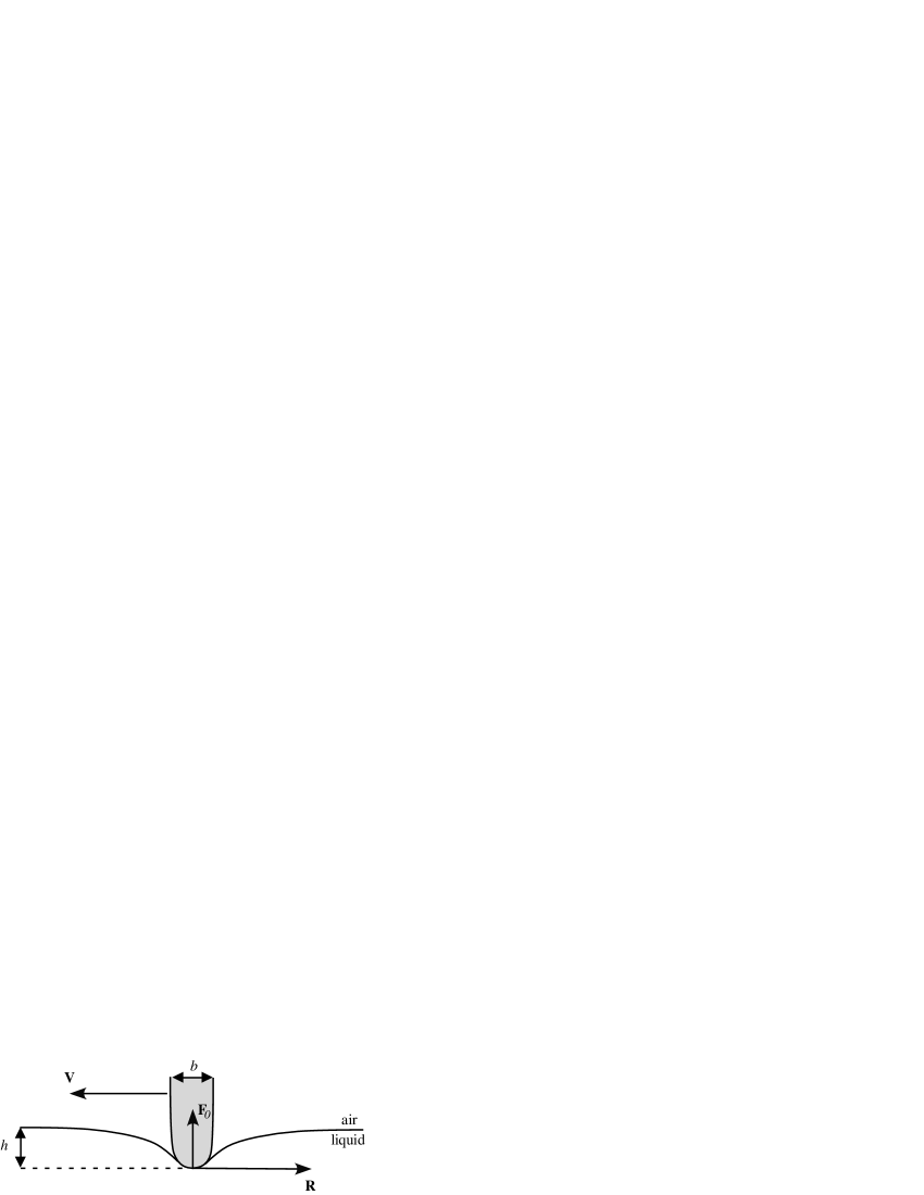
Figure 1: We study the behavior of a hydrophobic moving object of characteristic size $b$ immersed at a depth $h$. The velocity of the object is $V$. We decompose the force exerted by the fluid on the object in a component orthogonal to the free surface ($F_{0}$) and a component parallel to it ($R$).

2 Model

We take the $x,y$ plane as the equilibrium surface of the fluid. The immersed object exerts a stress at the fluid surface that can be considered equivalent to a pressure field $p$ [9] that travels over the surface with a velocity $V$ in the $x$ direction. We assume $\hat{p}$ (the Fourier transform of $p$) to be of the form:

$$\hat{p}(k_{x},k_{y})=F_{0}\hat{\phi}(k),$$ (2)

where $k=\sqrt{k_{x}^{2}+k_{y}^{2}}$ and $\hat{\phi}(0)=1$. In this case, $\hat{p}$ is isotropic [10] and $F_{0}$ is the total vertical force exerted on the fluid.

Within the framework of Rayleigh’s linearized theory of capillary-gravity waves, the Fourier transform $\hat{\xi}({\mathbf{k}})$ of the free surface displacement $\xi({\bf r})$ is related to the pressure field through [11]:

$$\hat{\xi}(k_{x},k_{y})=-F_{0}\frac{k}{\rho}\left(\frac{\hat{\phi}(k)}{\omega_{0}^{2}(k)-4\nu^{2}k^{3}q+(2\nu k^{2}-i{\mathbf{V}}\cdot{\mathbf{k}})^{2}}\right),$$ (3)

where $\omega_{0}^{2}(k)=gk+\gamma k^{3}/\rho$ is the free dispersion relation, $q^{2}=k^{2}-i{\mathbf{k}}\cdot{\mathbf{V}}/\nu$ and $\nu=\eta/\rho$ is the kinematic viscosity of the fluid.

Let us suppose the object is located at the origin of the moving frame. If $h$ is its depth, the free surface displacement $\xi$ must be $-h$ under the pinpoint (here we suppose the object sufficiently hydrophobic and $h$ not to large so that the pinpoint does not pierce the surface). This leads to the following normalization condition:

$$\xi({\mathbf{0}})=\int\frac{{\rm d}^{2}k}{(2\pi)^{2}}\,\hat{\xi}({\mathbf{k}})=-h.$$ (4)

The value of $h$ as a function of $F_{0}$ can be readily calculated using equations (3) and (4):

$$h=\Xi(V)F_{0},$$ (5)

with

$$\Xi(V)=\int\frac{{\rm d}^{2}k}{(2\pi)^{2}}\frac{k}{\rho}\left(\frac{\hat{\phi}(k)}{\omega_{0}^{2}(k)-4\nu^{2}k^{3}q^{2}+(2\nu k^{2}-i{\mathbf{V}}\cdot{\mathbf{k}})^{2}}\right).$$ (6)

Finally, the drag-force $\mathbf{R}$ is calculated by simply integrating the pressure force over the free surface [12].

$${\mathbf{R}}=-\int{\rm d}^{2}r\,p({\mathbf{r}}){\mathbf{\nabla}}\xi({\mathbf{r}})=-\int\frac{{\rm d}^{2}k}{(2\pi)^{2}}\,i{\mathbf{k}}\hat{p}^{*}({\mathbf{k}})\hat{\xi}({\mathbf{k}}).$$ (7)

This yields, using the explicit expression (3) for $\hat{\xi}$,

$${\mathbf{R}}=F_{0}^{2}{\mathbf{\Lambda}}(V),$$ (8)

with

$${\mathbf{\Lambda}}(V)=\int\frac{{\rm d}^{2}k}{(2\pi)^{2}\rho}\left(\frac{ik{\mathbf{k}}|\hat{\phi}(k)|^{2}}{\omega_{0}^{2}(k)-4\nu^{2}k^{3}q^{2}+(2\nu k^{2}-i{\mathbf{V}}\cdot{\mathbf{k}})^{2}}\right).$$ (9)

According to equation (8), the integral $\mathbf{\Lambda}$ describes the fixed-force behaviour of the wave-resistance. Due to the symmetry of $\hat{\phi}$, $\mathbf{\Lambda}$ is parallel to $\mathbf{V}$ and we shall henceforth set ${\mathbf{\Lambda}}=\Lambda{\mathbf{u}}$, where ${\mathbf{u}}={\mathbf{V}}/V$ is the unit vector parallel to the velocity of the object. The authors of [5] studied the properties of $\Lambda$ in the case of a non-viscous fluid for which they showed that:

(a) $\Lambda=0$ for $V<V_{\rm c}$;

(b) $\Lambda$ is discontinuous for $V\rightarrow V_{\rm c}^{+}$, with

$$\lim_{V\rightarrow V_{\rm c}^{+}}{\Lambda}=\Lambda_{\rm c}=\frac{1}{2\sqrt{2}}\frac{\kappa}{\gamma};$$ (10)

(c) in the large velocity limit

$$\Lambda\sim\frac{2\rho V^{2}}{3\pi\gamma^{2}}.$$ (11)

In the case of a fixed depth analysis, $F_{0}$ becomes a function of $V$. Using equations (5), we can rewrite the wave-resistance as

$${\mathbf{R}}=h^{2}\frac{{\mathbf{\Lambda}}(V)}{\Xi^{2}(V)}.$$ (12)

In general we have to rely on numerics to calculate the integrals $\Xi$ and $\Lambda$. Typical results are presented on Figure 2 for an objet of size 0.1 mm immersed in water, and for a step-like function $\hat{\phi}$ equal to 1 for $k<1/b$ and $0$ otherwise.

We first observe on Fig. (2-a) that $\Xi$ increases sharply near the threshold. This leads to two rather different behaviours for $\Lambda$ and $R$ as shown on Fig. (2-b): while $\Lambda$ exhibits a discontinuity close to $V=V_{\rm c}$ [13], the fixed-depth wave-drag $R=\Lambda/\Xi^{2}$ cancels smoothly at the critical velocity.

Figure 2: (a) Numerical calculation of the dimensionless integral $\bar{\Xi}=\Xi(V)/\Xi(0)$. (b) Comparison of $\bar{\Lambda}(V)=\Lambda(V)/\Lambda_{\rm c}$ (dashed line) and $\bar{R}=\bar{\Lambda}/\bar{\Xi}^{2}$ (full line) describing respectively the fixed-force and fixed-depth behaviour of the wave-resistance. We clearly see that contrary to the fixed-force analysis, the fixed-depth calculation does not yield any discontinuity at the threshold. Here $\nu=10^{-6}~{}{\rm m^{2}\cdot s^{-1}}$, $\gamma=72~{}{\rm mN\cdot m^{-1}}$, $\rho=1000~{}{\rm kg\cdot m^{-3}}$ and $b=0.1~{}{\rm mm}$.

3 Inviscid flow

The characteristic features displayed by the plots of Fig. 2 can be captured by a zero-viscosity analysis. Setting $\nu=0$, equation (6) can be simplified as:

$$\Xi={\cal P}\int\frac{{\rm d}^{2}k}{(2\pi)^{2}}\frac{k}{\rho}\left(\frac{\hat{\phi}(k)}{\omega_{0}^{2}(k)-({\mathbf{k}}\cdot{\mathbf{V}})^{2}}\right),$$ (13)

where $\cal P$ denotes the Cauchy principal value of the integral. The integral is calculated in polar coordinates $(k,\theta)$, where $\theta$ is the angle of $\mathbf{k}$ with respect to ${\mathbf{V}}$. Introducing the function $G$ defined by:

$$G(k)={\cal P}\int_{0}^{2\pi}\frac{{\rm d}\theta}{2\pi}\left(\frac{1}{m_{k}^{2}-2{\cal M}^{2}\cos^{2}(\theta)}\right),$$ (14)

where $m_{k}^{2}=k/\kappa+\kappa/k$ and ${\cal M}=V/V_{\rm c}$ is the “Mach” number, equation (13) can then be rewritten as:

$$\Xi=\frac{1}{\gamma\kappa}\int_{0}^{\infty}\frac{{\rm d}k}{2\pi}\hat{\phi}(k)G(k).$$ (15)

Using the residue theorem [14], we get:

$$G(k)=\frac{1}{\sqrt{m_{k}^{2}(m_{k}^{2}-2{\cal M}^{2})}}\,\Theta(m_{k}^{2}-2{\cal M}^{2}),$$ (16)

where $\Theta$ the is the Heaviside step-function. The variations of $m_{k}^{2}$ with $k$ are plotted on Fig. 3: $m_{k}^{2}$ reaches its minimum value $(m_{k}^{2})_{\rm min}=2$ for $k=\kappa$. It shows that equation $2{\cal M}^{2}-m_{k}^{2}=0$ has two solutions $k_{1}$ and $k_{2}$, with $k_{1}<\kappa<k_{2}$, if $V$ is larger than the critical velocity $V_{\rm c}$, and none if $V<V_{\rm c}$.

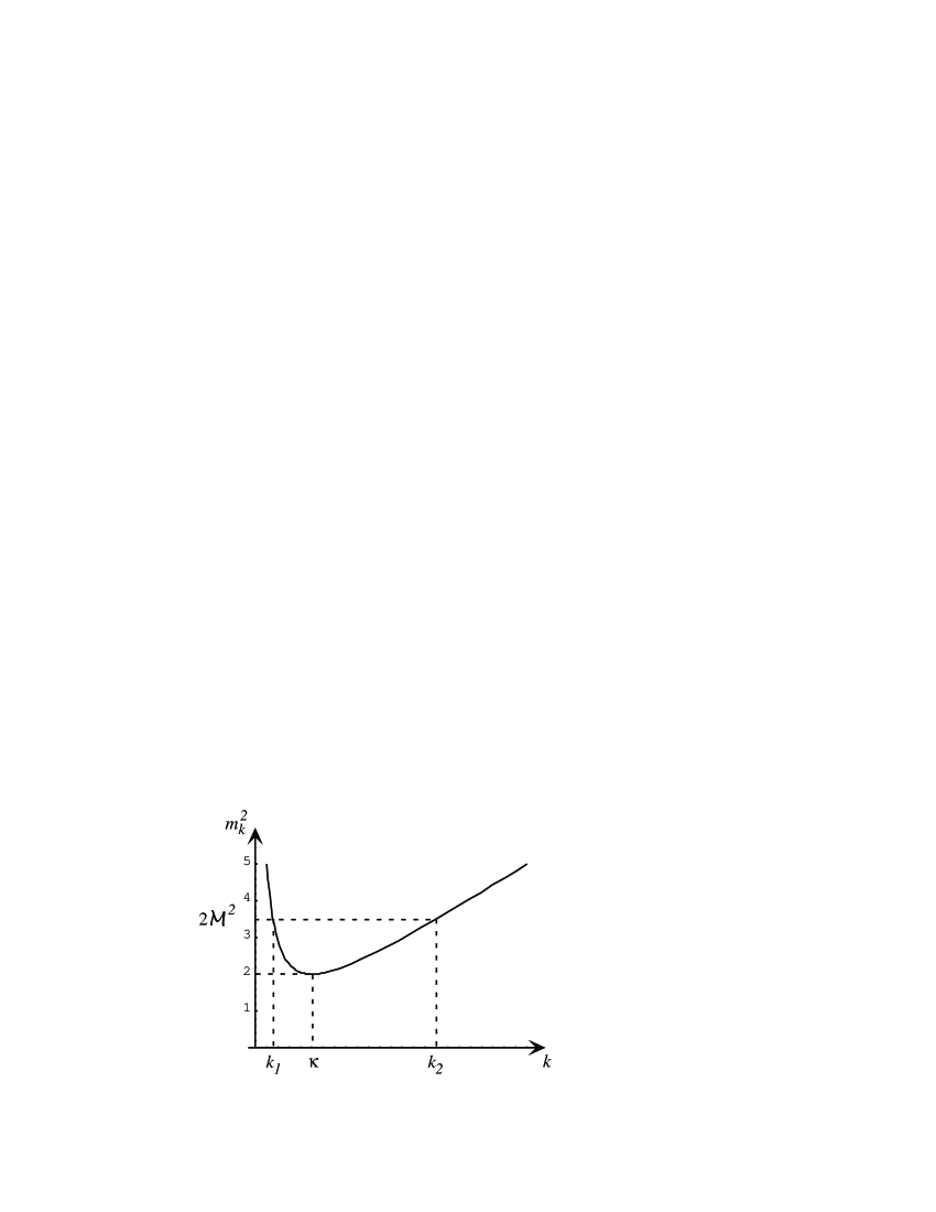
Figure 3: Variations of $m_{k}^{2}$ (see text) with k. Since $m_{k}^{2}$ reaches a minimum for $k=\kappa$ with $m_{\kappa}^{2}=2$, equation $m_{k}^{2}=2{\cal M}^{2}$ presents solutions for ${\cal M}>1$. In this case, there are two possible values $k_{1}$ and $k_{2}$ with $k_{1}<\kappa<k_{2}$.

For $V>V_{\rm c}$, $\Xi$ evaluates to

$$\Xi=\frac{1}{\gamma\kappa}\left[\int_{0}^{k_{1}}\frac{{\rm d}k}{2\pi}\frac{\hat{\phi}(k)}{\sqrt{m_{k}^{2}(m_{k}^{2}-2{\cal M}^{2})}}+\int_{k_{2}}^{\infty}\frac{dk}{2\pi}\frac{\hat{\phi}(k)}{\sqrt{m_{k}^{2}(m_{k}^{2}-2{\cal M}^{2})}}\right].$$ (17)

The above integrals can be calculated in the two limiting cases ${\cal M}\approx 1$ (i.e. $V\approx V_{\rm c}$) and ${\cal M}\gg 1$ (i.e. $V\gg V_{\rm c}$).

For large $\cal M$, the integrals are restricted to either large or small values of $k$. If $\hat{\phi}$ vanishes faster than $1/k$ for large $k$, we can show that the small $k$ contribution dominates. In this region, the dispersion relation is dominated by gravity waves, so that we can approximate $m_{k}^{2}$ by $k/\kappa$. A straightforward calculation then yields the following asymptotic expansion for $\Xi$:

$$\Xi\sim\frac{1}{6\pi\gamma}\left(\frac{V_{\rm c}}{V}\right)^{4}.$$ (18)

Combining this result with (11) and 12, we get:

$$R\sim 12\pi\rho h^{2}\frac{V^{10}}{V_{\rm c}^{8}}.$$

Let’s now focus on the case $V$ close to $V_{\rm c}$. We set:

$$\widetilde{\Xi}_{1}=\int_{0}^{k_{1}}\frac{{\rm d}k}{2\pi}\frac{\hat{\phi}(k)}{\sqrt{m_{k}^{2}(m_{k}^{2}-2{\cal M}^{2})}},$$

and

$$\widetilde{\Xi}_{2}=\int_{k_{2}}^{\infty}\frac{{\rm d}k}{2\pi}\frac{\hat{\phi}(k)}{\sqrt{m_{k}^{2}(m_{k}^{2}-2{\cal M}^{2})}}.$$

Using the fact that $k_{1}$ and $k_{2}$ are the roots of $m_{k}^{2}=2{\cal M}^{2}$, we can rewrite $\widetilde{\Xi}_{1}$ as:

$$\widetilde{\Xi}_{1}=\int_{0}^{k_{1}}\frac{{\rm d}k}{2\pi}\frac{k\hat{\phi}(k)}{\sqrt{(k^{2}/\kappa^{2})(k-k_{1})(k-k_{2})}}.$$

When $V\rightarrow V_{\rm c}$, the $(k-k_{1})(k-k_{2})$ term cancels in $k=\kappa$. Since all other terms are regular, we can write at the leading order:

$$\widetilde{\Xi}_{1}\sim\kappa\frac{\hat{\phi}(\kappa)}{\sqrt{2}}\int_{0}^{k_{1}}\frac{{\rm d}k}{2\pi}\frac{1}{\sqrt{(k-k_{1})(k-k_{2})}}.$$

This latter integral is readily calculated and gets a very simple form in the limit $V\rightarrow V_{\rm c}$:

$$\widetilde{\Xi}_{1}\sim\kappa\frac{\hat{\phi}(\kappa)}{\sqrt{2}}\ln\left(k_{2}-k_{1}\right)\sim\kappa\frac{\hat{\phi}(\kappa)}{2\sqrt{2}}\ln\left({\cal M}-1\right).$$

Since $m_{k}^{2}$ is invariant by the transformation $k/\kappa\rightarrow\kappa/k$, we see that $\Xi_{1}$ and $\Xi_{2}$ have the same asymptotic behaviour for $V\rightarrow V_{\rm c}$. In this limit we have $\Xi=\left(\widetilde{\Xi}_{1}+\widetilde{\Xi}_{2}\right)/\gamma\kappa\approx 2\widetilde{\Xi}_{1}/\gamma\kappa$, hence:

$$\Xi\sim\frac{1}{2\pi\sqrt{2}\gamma}\,\hat{\phi}(\kappa)\ln\left({\cal M}-1\right).$$ (19)

In the case of an object of size $b$, the width of $\hat{\phi}$ is about $1/b$. If we choose $b$ much smaller than the capillary length $\kappa^{-1}$, we can approximate $\hat{\phi}(\kappa)$ by $\hat{\phi}(0)=1$. In this limit, equation (19) takes the following form:

$$\Xi\sim\frac{1}{2\pi\sqrt{2}\gamma}\ln\left({\cal M}-1\right)\sim\frac{1}{2\pi\sqrt{2}\gamma}\ln\left(\frac{V-V_{\rm c}}{V_{\rm c}}\right).$$ (20)

If we combine equations (10) and (20), we see that slightly above the threshold, the wave-resistance behaves like:

$$R\sim\frac{4\pi^{2}}{\sqrt{2}}\left(\frac{\gamma\kappa h^{2}}{\ln^{2}\left(V/V_{\rm c}-1\right)}\right).$$ (21)

Equation (21) constitutes the main result of this paper. First, we notice that for small objects this relation is, as expected, independent of the actual shape of the pressure field. Second, and more important, it shows the wave resistance $R$ cancels out at $V=V_{\rm c}$. This smearing is due to the cancellation of the vertical force $F_{0}$ near the threshold that we get from the behaviour of $\Xi$.

4 Conclusion

In this paper we have shown that in a fixed-depth situation the discontinuity of the drag-force calculated in [5] vanishes and is replaced by a smooth variation, in accordance with the experimental results found in [7]. A quantitative comparison between the present analysis and the data of Ref. [7] is however more involved since experiments from [7] were performed in narrow channel geometry [15] with objects of size comparable with the capillary length. To recover the scaling relation observed experimentally, it would also be necessary to take into account both the variations of the shape of $\hat{\phi}$ with $V$ and the reflections of the waves on the walls of the channel. The present study suggests nevertheless that to fully test relation (1), experiments need to be devised that would measure both $R$ and $F_{0}$.

- [1] J. Lighthill, in Waves in Fluids (Cambridge University Press), 1978.
- [2] Lord Kelvin, Proc. Roy. Soc. London A, 42, 80 (1887).
- [3] For a review, see L. Debnath in Nonlinear Water Waves (Academic Press Inc., San Diego), 1994.
- [4] Note that for a viscous fluid, the moving perturbation is also subjected to the usual Stokes drag, for both and .
- [5] E. Raphaël and P.G. de Gennes, Phys. Rev. E, 53, 3448 (1996).
- [6] J. Browaeys, J.-C. Bacri, R. Perzynski and M. Shliomis, Europhys. Lett. 53, 209 (2001).
- [7] T. Burghelea and V. Steinberg, Phys. Rev. Lett. 86, 2557 (2001).
- [8] Shu-Ming Sun and J. Keller, Phys. Fluids 13, 2146 (2001).
- [9] Not that this assumption is not entirely correct in the presence of viscosity since it leads to a slip of the object with respect to the fluid surface. In this case, a force field parallel to the free surface should be added to take into account the viscous drag. However, this new term leads to the well known Stokes drag, that can substracted from experimental results, and so can be omitted in our analysis.
- [10] This latter hypothesis is not too restrictive in the case of very small objects for which the actual shape is not relevant.
- [11] This generalizes the 2D result of D. Richard and E. Raphaël, Europhys. Lett. 48, 53 (1999).
- [12] T.H. Havelock, Proc. Roy. Soc. Lond., A95, 354 (1918).
- [13] For an inviscid fluid, this increase is actually a discontinuity. For high viscosities, we have observed no noticeable accident of for close to .
- [14] See e.g. K.F. Riley, M.P. Hobson and S.J. Bence in Mathematical Methods for Physics and Engineering, (Cambridge University Press.), 1998.
- [15] V. Steinberg, private communication, and preprint submitted to Phys. Rev. E (2002).