Long term persistence in the sea surface temperature fluctuations

Roberto A. Monetti⁽¹⁾ ¹¹1Present address: Center for Interdisciplinary Plasma Science (CIPS), Max-Planck-Institut für extraterrestrische Physik, Giessenbachstr. 1, 85749 Garching, Germany. , Shlomo Havlin⁽¹⁾, and Armin Bunde⁽²⁾
(1) Minerva Center and Department of Physics
Bar-Ilan University, Ramat-Gan 52900, Israel
(2) Institut für Theoretische Physik III
Justus-Liebig-Universität Giessen
Heinrich-Buff-Ring 16, 35392 Giessen, Germany

Abstract

We study the temporal correlations in the sea surface temperature (SST) fluctuations around the seasonal mean values in the Atlantic and Pacific oceans. We apply a method that systematically overcome possible trends in the data. We find that the SST persistence, characterized by the correlation $C(s)$ of temperature fluctuations separated by a time period $s$ , displays two different regimes. In the short-time regime which extends up to roughly $10$ months, the temperature fluctuations display a nonstationary behavior for both oceans, while in the asymptotic regime it becomes stationary. The long term correlations decay as $C(s)\sim s^{-\gamma}$ with $\gamma\sim 0.4$ for both oceans which is different from $\gamma\sim 0.7$ found for atmospheric land temperature.

1 Introduction

The oceans cover almost three quarters of the Earth’s surface and have the greatest capacity to store heat. Thus, they are able to regulate the temperature on land even in sites located far away from the coastline. This property of the oceans suggests that they may posses a strong temperature persistence, i.e. a strong tendency that the water temperature of a particular day will remain the same the next day. Persistence can be characterized by the auto-correlation function $C(s)$ of temperature variations separated by a time period $s$ . Recently, quantitative studies of the persistence in atmospheric land temperatures revealed that atmospheric land temperature fluctuations exhibit long-range power law correlations $C(s)\sim s^{-\gamma}$ with $\gamma\approx 0.70$ [Koscielny-Bunde et al., 1996; Koscielny-Bunde et al., 1998; Pelletier, 1997; Pelletier et al., 1997; Talkner et al., 2000]. In this Letter, we study the persistence in sea surface temperature (SST) records at many sites in the Atlantic and Pacific oceans using the detrended fluctuation analysis (DFA) method [Peng et al., 1994; Kantelhardt et al., 2001]. We find that for all time scales the SST fluctuations exhibit stronger correlations than atmospheric land temperature fluctuations. The long term persistence of the SST is characterized by a correlation exponent $\gamma\sim 0.4$ for both oceans.

We have analyzed both types of SST data sets that are available, the monthly SST for the period $1856-2001$ and the weekly SST for the period $1981-2001$ . For the period 1856-1981, the monthly SST data sets were obtained by Kaplan et al. [Kaplan et al., 1998] who used optimal estimation in space applying 80 empirical orthogonal functions to interpolate ship observations of the United Kingdom Meteorological Office database [Parker et al., 1994]. After 1981, the monthly data correspond to the projection of the National Center for Environmental Prediction (NCEP) optimal interpolation (OI) analysis [Reynolds et al., 1993; Reynolds et al., 1994]. The weekly SST’s also correspond to the NCEP OI analysis. The data are freely available from http://ingrid.ldeo.columbia.edu/SOURCES/.

2 The Method

We focus on the temperature fluctuations around the periodical seasonal trend. In order to remove the periodical trend, we first determine the mean temperature $\langle T_{a}\rangle$ for each month/week by averaging over all years in the time series. Then, we analyze the temperature deviations $\Delta T_{i}=T_{i}-\langle T_{a}\rangle$ from these mean values. The persistence in the temperature fluctuations can be characterized by the auto-correlation function,

C(s)\equiv\langle\Delta T_{i}\Delta T_{i+s}\rangle=\frac{1}{N-s}\sum_{i=1}^{N-s}\Delta T_{i}\Delta T_{i+s},

(1)

where $N$ is the length of the record and $s$ is the time lag. A direct calculation of $C(s)$ is hindered by the level of noise present in the finite temperature series and by possible nonstationarities in the data. To reduce the noise, we study the temperature profile function,

Y_{k}=\sum_{i=1}^{k}\Delta T_{i}.

(2)

We can consider the profile $Y_{k}$ as the position of a random walker on a linear chain after $k$ steps. According to the random walk theory, the fluctuations $F(s)$ of the profile in a given time window of length $s$ are related to the correlation function $C(s)$ . For the relevant case of long-range power law correlations,

C(s)\sim s^{-\gamma},\hskip 28.45274pt0<\gamma<1,

(3)

the fluctuations increase as a power law [Barabasi et al., 1995; Shlesinger et al., 1987],

F(s)\sim s^{\alpha},\hskip 28.45274pt\alpha=1-\gamma/2.

(4)

For uncorrelated data ( $\gamma\geq 1$ ), we have $\alpha=1/2$ . To find how the fluctuations scale with $s$ , we divide the profile into non-overlapping intervals of length $s$ . We calculate the square fluctuations $F^{2}_{\nu}(s)$ in each interval $\nu$ and obtain $F(s)$ by averaging over all intervals, $F(s)\equiv\langle F^{2}_{\nu}(s)\rangle^{1/2}$ . Here, we use two methods that differ in the way fluctuations are measured. In the fluctuation analysis (FA), the square of the fluctuations is defined as $F^{2}_{\nu}(s)=(Y_{(\nu+1)s}-Y_{\nu s})^{2}$ where $Y_{\nu s}$ and $Y_{(\nu+1)s}$ are the values of the profile at the beginning and the end of each segment $\nu$ , respectively. In the detrended fluctuation analysis, we determine in each interval the best polynomial fit of the profile and define $F_{\nu}(s)$ as the variance between the profile and the best fit in the intervals. Different orders $n$ of DFA (DFA1, DFA2, etc) differ in the order of the polynomial used in the fitting procedure. By construction, FA is sensitive to any kind of trend and thus equivalent to the Hurst and the power spectrum analyses. In contrast, DFA $n$ removes a polynomial trend of order $n-1$ in the temperature record and thus, it is superior to the conventional methods.

To characterize the persistence, we have applied the FA and DFA methods to $36$ ( $46$ ) monthly SST records and $64$ ( $35$ ) weekly SST records in the Atlantic (Pacific) ocean.

3 Results and Discussion

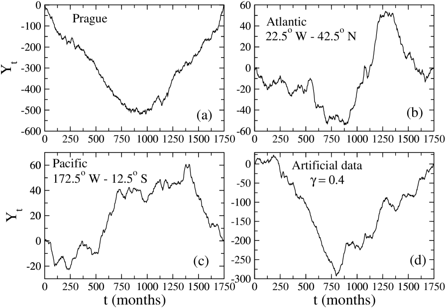
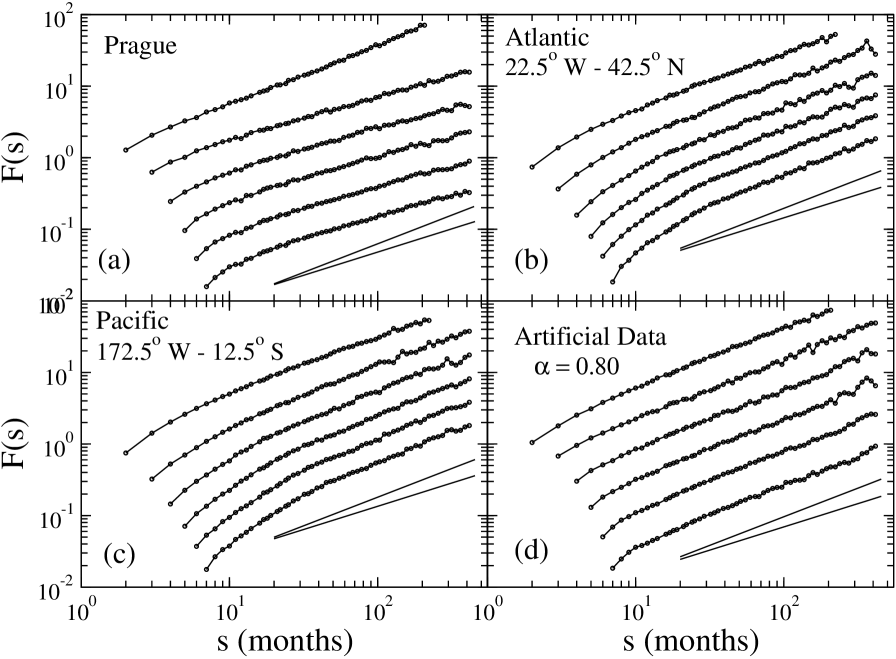
Figure 1(a-c) show three typical plots of the monthly temperature profile function $Y_{t}$ for a land station (Prague), a site in the Atlantic ocean, and a site in the Pacific ocean, respectively. Parabolic-like profile functions which are concave (convex) may indicate the presence of a positive (negative) linear trend (see Eq. 2). However, Fig. 1(d) illustrates that pure correlated data may also lead to parabolic-like profile functions. Trends and correlations can be distinguished and characterized by comparing the FA and DFA results [Kantelhardt et al., 2001; Govindan et al., 2001]. Figure 2 shows log-log plots of the FA and DFA curves for the profiles shown in Fig. 1. Figure 2(a) shows that at large times Prague temperature fluctuations display a power law behavior. The fluctuation exponent obtained from the FA (0.81) is greater than the values given by the DFA1-5 (0.65). This difference is probably due to the effect of the well known urban warming of Prague. The fluctuation exponent $\alpha\approx 0.65$ is consistent with the earlier finding, where the whole Prague record (218 years) has been analyzed [Koscielny-Bunde et al., 1996; Govindan et al., 2001]. Figure 2(a) shows that the FA (and the similar Hurst and power spectrum methods) may lead to spurious results because of the presence of trends, yielding a large overestimation of long range correlations. Figure 2(d) shows the FA and DFA results for the artificial data used in Fig. 1(d). Although the profile function suggested the presence of a trend, the FA and the DFA show no evidence of any trend (see references [Hu et al., 2001; Vjushin et al., 2001]). Figures 2(b) and 2(c) show the FA and DFA results for two typical sites in the Atlantic and Pacific oceans, respectively. Here, for long time scales, FA and DFA curves are straight lines with roughly the same fluctuation exponent $\alpha\sim 0.8$ . This shows that (a) trends do not falsify the FA result and therefore may be regarded as much less important than for Prague temperatures, and (b) long range correlations also occur in SST’s. These correlations are stronger than the correlations in the atmospheric land temperatures, since the fluctuation exponent $\alpha\sim 0.8$ corresponds to a correlation exponent $\gamma\sim 0.4$ . As in the case of atmospheric land temperatures [Koscielny-Bunde et al., 1996], the range of this persistence law seems to exceed one decade and is possible even longer than the range of the SST series considered.

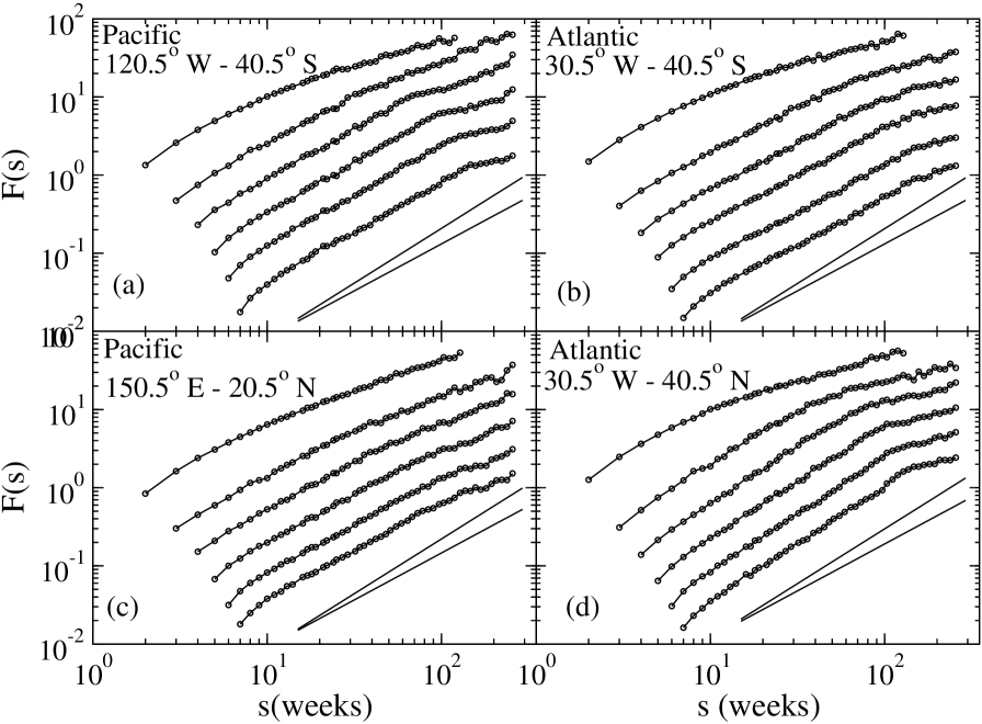
In contrast to Prague, there is a pronounced short-time regime which ends roughly at 10 months. This regime can be better revealed by the analysis of the weekly SST series. Figure 3 shows the FA and DFA results for $4$ sites in the Atlantic and Pacific oceans. This figure shows that for short times, the SST exhibits a persistence which is considerably stronger than both the SST long term persistence and the atmospheric land temperature persistence. The typical SST short-time fluctuation exponent is $\alpha\approx 1.2$ . However, in the northern Atlantic (latitudes from 30^o to 50^o north) we have found even higher fluctuation exponents. Figure 3(d) shows the results for a typical site in the northern Atlantic, yielding $\alpha\approx 1.4$ . The fact that $\alpha$ is above $1$ means that the variance of the original temperature fluctuations in a time window $s$ increases as $s^{\alpha-1}$ , i.e. as $s^{0.4}$ in the Northern Atlantic and $s^{0.2}$ in the rest of the oceans for time scales below $10$ months. This non-stationary behavior must be contrasted with the atmospheric land temperature fluctuations where the variance stays constant and the persistence decays with a nearly universal exponent $\gamma\sim 0.7$ . Non-stationary behavior has also been found in the analysis of marine stratocumulus cloud base height records [Kitova et al., 2002].

We like to suggest the following interpretation for the difference in the short-term persistence between the Northern Atlantic and the rest of the oceans. In the northern Atlantic, the dominant mode of interannual variability in the atmospheric circulation is the North Atlantic Oscillation (NAO) [Hurrell, 1995; Thompson et al., 1998]. This weather phenomenon highly influences the climate in the eastern part of North America and northern Europe and is usually characterized by the NAO index which is based on the normalized difference in sea level pressure between Ponta Delgada, Azores (26^o W, 38^o N) and Akureyri, Iceland (18^o W, 66^o N). The NAO index varies from positive values in winters to negative values in other seasons. During the last twenty years, the NAO index has displayed a persistent and exceptionally strong positive phase [Hurrell, 1995]. Since the sea level pressure and the SST are coupled variables, it is likely that the observed persistence in the NAO index is also revealed by the greater fluctuation exponent found in SST’s in the same period.

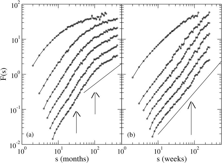
In order to find how representative the values of the fluctuation exponents are, we have studied the distribution of the short- and long-term exponents for both the Atlantic and the Pacific ocean. For the long-term exponents, we exclude those sites in the tropical Pacific region where the El Niño southern oscillation (ENSO) takes place [Tziperman et al., 1994; Cane et al., 1986]. The reason for this is that ENSO is a cyclic phenomenon which warms the east equatorial Pacific ocean every three to six years. This cycle cannot be detrended and strongly affects the DFA results on scales between $2$ and $20$ years. At small scales below $2$ y, higher order DFA is able to remove the trend. At larger scales, well above $20$ y, the oscillations cancel each other and the fluctuations again become dominant. However, for obtaining reliable results on the scaling above $20$ y, we need data covering far more than $200$ y. Those data are not available, and therefore we cannot specify the long-term exponents in the ENSO region. Figure 4 shows the results from our fluctuation analysis for a typical site in the tropical Pacific region, both for the weekly and the monthly data. Below $2$ y, the exponent is close to $1.2$ , and is therefore similar to the short-term exponent for the rest of the sites. Above $2$ y, the influence of the oscillations shows up. First, the exponent crosses over to a larger value, and then, above $3$ y for DFA1 and above $8$ y for DFA5, crosses over to a very low value. This effect of oscillations on the DFA analysis was recently described in [Kantelhardt et al., 2001; Hu et al., 2001]. We expect that at much larger scales, the exponent will gradually increase approaching the value $\alpha\sim 0.8$ as for the sites outside the ENSO regime. However, the data sets are too short to observe this effect.

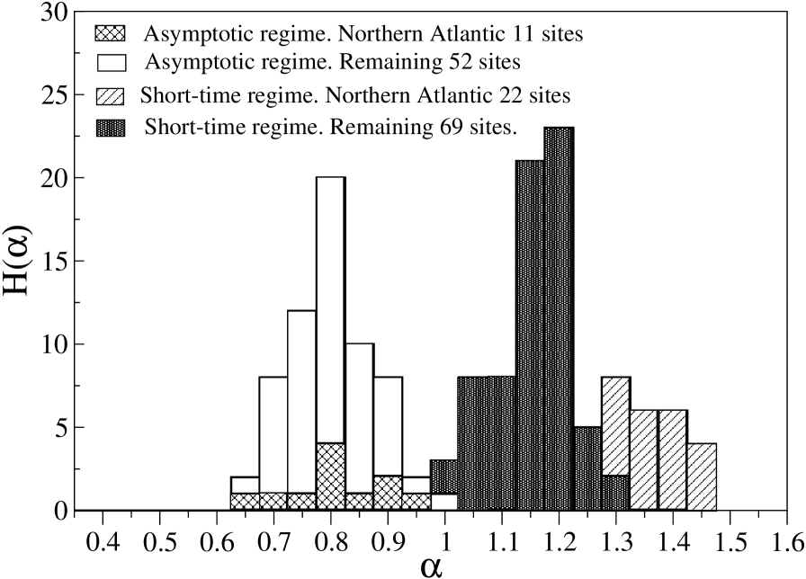
Figure 5 summarizes our results for the short- and long-term exponents for both the Atlantic and the Pacific oceans. As said before, for the short-term exponents, sites in the ENSO region are included in the histogram, while for the long-term exponents they are not. The histogram shows that the short term exponents for the Northern Atlantic ( $\alpha=1.38\pm 0.04$ ) where the NAO takes place, are well distinct from the short term exponents of the remaining sites ( $\alpha=1.17\pm 0.08$ ). For the asymptotic long-term exponents ( $\alpha=0.8\pm 0.08$ ) there is not such a clear distinction between the Northern Atlantic area and the rest.

4 Conclusions

In summary, we have studied the persistence of the sea surface temperature in the Atlantic and Pacific oceans. We found that, in contrast to land stations, there exist two pronounced scaling regimes. In the short-time regime that roughly ends at 10 months, the fluctuations of the temperature profile, in a given time window $s$ , scales as $s^{\alpha}$ , with an exponent $\alpha$ in the northern Atlantic ( $\alpha\sim 1.4$ ) that differs from the rest of the oceans ( $\alpha\sim 1.2$ ). This behavior is well distinct from the temperature fluctuations on land, where $\alpha$ is close to $0.65$ above typically 10 days. The fact that in the short-time regime $\alpha$ is well above $1$ points to an intrinsic non-stationary behavior where the variance of the original temperature fluctuations in a time window of size $s$ increases with $s$ as $s^{\alpha-1}$ . This non-stationary behavior crosses over to stationary behavior at time scales above $10$ months, where now the fluctuation exponent reaches the value $\alpha\sim 0.8$ for all sites considered in both oceans. This result reveals that pronounced long term correlations govern the SST, with an exponent $\gamma\sim 0.4$ . The persistence in the SST is due to the capacity of the oceans to store heat [Levitus et al., 2001]. The oceans also contribute to the temperature persistence on land but in a less direct way, i.e. by coupling to the atmosphere. This may be the reason why the persistence of atmospheric land temperatures is less pronounced. In the view of our results, it is interesting that coastline stations (like Melbourne, Sidney, and New York) show the same persistence exponent like inland stations (like Prague and Luling). Finally, we also like to emphasize that the scaling laws we find here may serve as further non-trivial test-bed for the state-of-the-art global climate models (see [Govindan R., 2002]).

Acknowledgments: We like to acknowledge financial support from CONICET (Argentina), the Israel Science Foundation and the Deutsche Forschungsgemainschaft.

References

[1] Koscielny-Bunde E., Bunde A., Havlin S., Roman H. E., Goldreich Y., Schellnhuber H.-J., Indication of a universal persistence law governing atmospheric variability, Phys. Rev. Lett., 81, 729–732, 1998.
[2] Koscielny-Bunde E., Bunde A., Havlin S., Goldreich Y., Analysis of daily temperature fluctuations, Physica A, 231, 393–396, 1996.
[3] Pelletier J. D., Analysis and modeling of the natural variability of climate, J. Climate, 10, 1331–1342, 1997.
[4] Pelletier J. D. and Turcotte D. L., J. Hydrology, 203, 198–208, 1997.
[5] Talkner P. and Webber R.O., Power spectrum and detrended fluctuation analysis: Application to daily temperatures, Phys. Rev. E, 62, 150–160, 2000.
[6] Peng C.-K., Buldyrev S.V., Havlin S., Simons M., Stanley H.E., Goldberger A.L., Mosaic Organization of DNA Nucleotides, Phys. Rev. E, 49, 1685–1689, 1994.
[7] Kantelhardt J.W., Koscielny-Bunde E., Rego H.H.A., Havlin S., Bunde A., Detecting long-range correlations with detrended fluctuation analysis, Physica A, 295, 441–454, 2001.
[8] Kaplan A., Cane M., Kushnir Y., Clement A., Blumenthal M., and Rajagopalan B., Analyses of global sea surface temperature 1856-1991, J. of Geophys. Res-Oceans, 103, 18567–18589, 1998.
[9] Parker D. E., Jones P. D., Folland C. K., and Bevan A., Interdecadal changes of Surface-Temperature since the late-19th-century, J. of Geophys. Res-Atmos, 99, 14373–14399, 1994.
[10] Reynolds R. and Marsico D., An Improved Real-Time Global Sea-Surface Temperature Analysis, J. Climate, 6, 114–119, 1993.
[11] Reynolds R. and Smith T., Improved Global Sea-Surface Temperature Analyses using Optimum Interpolation, J. Climate, 7, 929–948, 1994.
[12] Barabasi A.-L and Stanley H. E., Fractal Concepts in Surface Growth (Cambridge University Press, 1995).
[13] Shlesinger M., West B., and Klafter J., Levy Dynamics of Enhanced Diffusion - Application to Turbulence, Phys. Rev. Lett., 58, 1100–1103, 1987.
[14] Govindan R. , Vjushin D., Brenner S., Bunde A. , Havlin S., and Schellnhuber H.-J., Long-range correlations and trends in global climate models: Comparison with real data, Physica A, 294, 239–248, 2001.
[15] Hu K., Ivanov P.Ch., Chen Z., Carpena P., and Stanley H. E., Effect of trends on detrended fluctuation analysis, Phys. Rev. E, 64, 011114, 2001.
[16] Vjushin D., Govindan R., Monetti R., Havlin S., and Bunde A., Scaling analysis of trends using DFA, Physica A, 302, 234–243, 2001.
[17] Kitova N., Ivanova K., Ausloos M., Ackerman T., Mikhalev M., Time dependent correlations in marine stratocumulus cloud base height records, Int. Jour. Mod. Phys. C, 13, 217–227, 2002.
[18] Hurrell J., Decadal Trends in the North-Atlantic Oscillation - Regional Temperatures and Precipitation, Science, 269, 676–679, 1995.
[19] Thompson D. and Wallace J., The Arctic Oscillation signature in the wintertime geopotential height and temperature fields, Geophys. Res. Lett., 25, 1297–1300, 1998.
[20] Tziperman E., Stone L., Cane M., and Jarosh H., Science, 264, 72–74, 1994.
[21] Cane M., Zebiak S., and Dolan S., Experimental Forecast of El-Nino, Nature, 321, 827–832, 1986.
[22] Levitus S, Antonov JI, Wang JL, Delworth TL, Dixon KW, and Broccoli AJ, Anthropogenic warming of Earth’s climate system, Science, 292, 267–270, 2001.
[23] Govindan R., Vjushin D., Brenner S., Bunde A., Havlin S., Schellnhuber H.-J., Global climate models violate scaling of the observed atmospheric variability, Phys. Rev. Lett., 89, 028501, 2002.

Refer to caption — Figure 1: Typical temperature profile functions for the last 146 years (monthly data). (a) Prague, (b) Atlantic ocean (22.5W, 42.5S), (c) Pacific ocean (172.5W, 12.5S), (d) Artificial correlated data with $\gamma=0.4$ .