A comparison of extremal optimization with flat-histogram dynamics for finding spin-glass ground states

Abstract

We compare the performance of extremal optimization (EO), flat-histogram and equal-hit algorithms for finding spin-glass ground states. The first-passage-times to a ground state are computed. At optimal parameter of $\tau=1.15$, EO outperforms other methods for small system sizes, but equal-hit algorithm is competitive to EO, particularly for large systems. Flat-histogram and equal-hit algorithms offer additional advantage that they can be used for equilibrium thermodynamic calculations. We also propose a method to turn EO into a useful algorithm for equilibrium calculations.

Keywords: extremal optimization. flat-histogram algorithm, equal-hit algorithm, spin-glass model, ground state.

1 Introduction

Optimization with methods motivated from real physical processes is an active field of research. Simulated annealing [1] and genetic algorithm [2] are two well-known examples. In particular, there have been a large variety of methods proposed to find spin-glass ground states [3, 4, 5, 6, 7, 8, 9, 10]. Recently, Boettcher and Percus [11, 12] introduced ‘extremal optimization’ (EO) inspired by models of self-organized criticality [13], which gave impressive performance.

Most of the heuristic optimization methods (including simulated annealing and genetic algorithm) are designed to find ground states only, thus it is not possible to give correct thermodynamics from a simulation. On the other hand, multi-canonical ensemble simulation [14], $1/k$-sampling [15], parallel tempering [16], and recent flat-histogram dynamics [17] are constructed for equilibrium thermodynamics, but can also be used as methods for optimization. A study of optimization by flat-histogram algorithm on the two-dimensional spin-glass model is carried out in ref. [18]. Unlike simulated annealing and other heuristic methods, we note that these methods do not have any adjustable parameters. It is useful to know the efficiencies of this second class of methods when used as an optimization tool.

In this paper, we make a comparative study of the extremal optimization and flat-histogram/equal-hit dynamics. We compare four algorithms: EO at $\tau=1$ with a continuous approximation in the probability of choosing a site, original EO at optimal value of $\tau=1.15$, single-spin-flip flat-histogram dynamics, and equal-hit algorithm with $N$-fold way. It is found that EO at the value $\tau=1.15$ is very good for both two- and three-dimensional Ising spin glasses. The equal-hit algorithm with $N$-fold way is also competitive. For large systems, equal-hit appears even slightly better than EO. It is useful to have the efficiency of EO but still give equilibrium results. To this end, we introduce a rejection step in EO, thus turning EO into an equilibrium simulation method.

2 Single-spin-flip algorithms

In the following, we specialize our discussion in the context of spin models, and particularly the spin-glass model [19]. The energy function is defined by

$$E(\sigma)=-\sum_{\langle i,j\rangle}J_{ij}\sigma_{i}\sigma_{j},$$ (1)

where the spin $\sigma_{i}$ takes on value $+1$ or $-1$ with $i$ varying over a hypercubic lattice in $d$ dimensions. The coupling constant $J_{ij}$ for each nearest neighbor pair $\langle i,j\rangle$ takes on a random value of $+J$ and $-J$ with equal probability. We impose a constraint $\sum_{\langle i,j\rangle}J_{ij}=0$. The spin glass is known to be one of the hardest problems [20] to find the state $\sigma$ that minimizes $E(\sigma)$.

A single-spin-flip with rejection is described by a Markov chain transition matrix of the form

$$W(\sigma\to\sigma^{\prime})=\delta_{N}(\sigma,\sigma^{\prime}){1\over N}a(\sigma\to\sigma^{\prime}),\qquad\sigma\neq\sigma^{\prime},$$ (2)

where $\delta_{N}(\sigma,\sigma^{\prime})=1$ if $\sigma^{\prime}$ is obtained from $\sigma$ by a single spin flip, and 0 otherwise. The factor $1/N$ represents the random selection of a spin, where $N$ ($=L^{d}$) is the number of spins. $a(\sigma\to\sigma^{\prime})$ is the flip rate. If we choose $a(\sigma\to\sigma^{\prime})$ according to Metropolis rate,

$$a(\sigma\to\sigma^{\prime})=\min\left(1,{f\bigl{(}E(\sigma^{\prime})\bigr{)}\over f\bigl{(}E(\sigma)\bigr{)}}\right),$$ (3)

we can realize equilibrium distribution with the probability of states distributed according to $f\bigl{(}E(\sigma)\bigr{)}$. Some choices are:

$$f(E)=\cases{\exp\bigl{(}-E/(k_{B}T)\bigr{)},&canonical ensemble;\cr 1/n(E),&multicanonical ensemble;\cr 1/\int_{-\infty}^{E}n(E^{\prime})dE^{\prime},&$1/k$ sampling,\cr}$$ (4)

where $T$ is temperature, $k_{B}$ is Boltzmann constant, and $n(E)$ is density of states at energy $E$.

Arbitrary choice of the flip rate $a(\sigma\to\sigma^{\prime})$ in general would not give one important property of the equilibrium systems, i.e., the microcanonical property that the probability distribution of the configuration $\sigma$ is a function of energy $E$ only. For example, the original broad histogram rate [21]

$$a(\sigma\to\sigma^{\prime})=\min\left(1,{N_{Z-k}(\sigma)\over N_{k}(\sigma)}\right),$$ (5)

and the random walk rate of Berg [22] do not have microcanonical property, where $N_{k}(\sigma)$ is the number of possible moves of class $k$ in the state $\sigma$; we associate a class for each site $i$ with a number from 0 to $Z$ ($=2d$) by a scaled energy change $k=\bigl{(}(E(\sigma^{\prime})-E(\sigma))/J+2Z\bigr{)}/4$, i.e.,

$$k={1\over 2}\sum_{j}(J_{ij}\sigma_{i}\sigma_{j}+1).$$ (6)

$N_{k}(\sigma)$ is the number of such sites having a class $k$.

The single-spin-flip version with rejection can be turned into a rejection-free $N$-fold way [23] simulation where a class is chosen with probability

$$P_{k}={a_{k}N_{k}(\sigma)\over A(\sigma)},\quad A(\sigma)=\sum_{k=0}^{Z}a_{k}N_{k}(\sigma),$$ (7)

where $a_{k}$ is $a(\sigma\to\sigma^{\prime})$ associated with an energy change indicated by class $k$. A spin in that class is picked up at random, and the flip is always accepted. Thermodynamic quantities need to be weighted by a factor $1/A(\sigma)$.

EO [11, 12] is somewhat related to $N$-fold way in the sense that a class is chosen with some probability $P_{k}$, and a spin in that class is picked up and always flipped. The EO algorithm can be stated as follows: we classify the site by its ‘fitness’ $k$. There are $Z+1$ possible values for $k$. In the general EO, the sites are sorted according to the fitness $k$. Since there are only a small number of possible values in the $\pm J$ spin-glass model, the sorting is not necessary. We simply make a list of sites in each category. We pick a class according to the probability $P_{k}$, and then choose a spin in that class and flip with probability one. The corresponding transition matrix is then

$$W(\sigma\to\sigma^{\prime})=\delta_{N}(\sigma,\sigma^{\prime})P_{k}{1\over N_{k}},\qquad\sigma\neq\sigma^{\prime}.$$ (8)

The original choice of EO is to take

$$P_{k}\propto\sum_{N_{0}+N_{1}+\cdots+N_{k-1}<i\leq N_{0}+N_{1}+\cdots+N_{k}}i^{-\tau},$$ (9)

with $\tau$ being a parameter of the algorithm. We define the standard EO to be a continuous approximation to the above sum at $\tau=1$ with the analytical expression by

$$P_{k}={1\over\ln(N+1)}\ln{1+\sum_{j=0}^{k}N_{j}\over 1+\sum_{j=0}^{k-1}N_{j}}.$$ (10)

The number 1 in the numerator and denominator are introduced somewhat arbitrarily to avoid divergence when the sum of $N_{k}$ is zero. An optimized EO will be the discrete version, Eq. (9), with $\tau$ that gives best performance; we use $\tau=1.15$ as recommended in ref [12]. To realize the power-law distribution, we generate an integer $i=\lfloor\xi^{1/(1-\tau)}\rfloor$, where $\xi$ is a uniformly distributed random number between 0 and 1, and pick a corresponding site $i$ ordered by the class. We have used $\lfloor\cdots\rfloor$ for the floor function.

3 Comparison of EO with flat-histogram and equal-hit algorithms

The flat-histogram algorithm [17, 24] is a special choice of the flip rate

$$a^{{\rm FH}}(\sigma\to\sigma^{\prime})=\min\left(1,{\langle N_{Z-k}(\sigma^{\prime})\rangle_{E^{\prime}}\over\langle N_{k}(\sigma)\rangle_{E}}\right),$$ (11)

where the angular brackets with subscript $E$ denote a microcanonical average of the quantity $N_{k}(\sigma)$ at energy $E$; the starting state $\sigma$ has energy $E$ and the final state $\sigma^{\prime}$ has energy $E^{\prime}$. This particular choice of the rate gives a flat distribution for the energy histogram, $H(E)=n(E)f(E)={\rm const}$, $n(E)$ is density of states. This is one way to realize multicanonical ensemble.

In the $N$-fold way equal-hit algorithm [24, 25], we perform the usual $N$-fold-way move (thus rejection-free) which is constructed from the following single-spin-flip rate:

$$a^{{\rm EQ}}(\sigma\to\sigma^{\prime})=\min\left(1,{\langle A\rangle_{E}\langle N_{Z-k}(\sigma^{\prime})\rangle_{E^{\prime}}\over\langle A\rangle_{E^{\prime}}\langle N_{k}(\sigma)\rangle_{E}}\right).$$ (12)

We note that $\langle A\rangle_{E}^{-1}=\langle 1/A\rangle_{N}$, where $\langle\cdots\rangle_{N}$ is average over the $N$-fold way samples. In equal-hit algorithm, it is guaranteed by construction that we change state in every move, and the distribution of the visits to different energies is flat.

Since the microcanonical averages used in the flip rates are not known before the simulation, we use running average to replace the exact microcanonical average. It appears that this is a valid approximation and should converge to the correct values for sufficiently long runs. For a truly exact algorithm (in the sense of realizing microcanonical property), it is sufficient with a two-pass simulation. The first pass uses a running average; in the second pass, we use a multicanonical rate determined from the first pass.

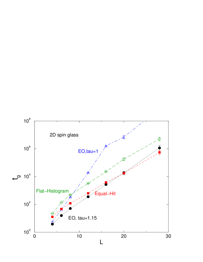
Figure 1: The average first-passage time $t_{g}$ in units of sweeps to find a ground state for four algorithms: standard EO (triangles), optimal EO (circles), flat-histogram (diamonds), and equal-hit (squares) for the two-dimensional spin-glass model. Over $10^{3}$ realization of random coupling samples are used for averaging for each algorithm and size.

Many different criteria are used to measure the effectiveness of an optimization algorithm, such as the fraction of cases for which ground states are found in a set of runs. The first-passage-time, the time in units of Monte Carlo sweeps that a ground state is found, starting with similar random configurations, should be a good measure of the algorithms’ efficiency. We consider sample average of the first-passage-time, although the distribution of it is also very useful. The computer CPU time is another useful criterion when comparing algorithms of very different types.

In the flat-histogram and equal-hit algorithms, we can sample positive as well as negative energies uniformly. In this study, we have restricted to the negative energy part, where moves to $E>0$ region are rejected. We compute the average time (first-passage time) for each lattice size and given algorithm in units of sweeps ($N=L^{d}$ basic moves) to find a ground state, starting from a random configuration of equal probability of spin up and spin down. For two-dimensional $\pm J$ spin glass, we determine the first-passage time $t_{g}$ by comparing the current value of energy with the exact value of ground state energy, obtained from the Spin Glass Server [26]. Thus the results are unbiased. The average first-passage time $t_{g}$ for the two-dimensional Ising spin-glass model is shown in Fig. 1. Over $10^{3}$ realization of random coupling samples are used for averaging for each algorithm and size.

Since the ground state energies are usually not known in three dimensions, we consider instead the time for finding the lowest energy for a fixed amount of sweeps $t$, averaged over the coupling constants with the constraint $\sum J_{ij}=0$. For any fixed running length $t$, results obtained are only a lower bound for $t_{g}$. We consider run lengths of $10^{4}$, $10^{5}$, $10^{6}$, etc, until the first-passage time converges for large $t$. This limiting time $t_{g}$ is reported for the three-dimensional Ising spin-glass model in Fig. 2.

To compare the efficiency of the four algorithms, the actual CPU times are also an important factor. For our implementation, it turns out that the optimized EO, standard EO, and $N$-fold way equal-hit all have about the same speed at 6 microsecond per spin flip on a 700 MHz Pentium, while the single-spin-flip flat-histogram algorithm takes 3 microsecond. There are several important features in this comparison, see Fig. 1. All of them have a first-passage time that grows rapidly with sizes. With the exception of the standard EO, they nearly have the same slope of about 6 on a double logarithmic scale. It is also interesting to compare the first-passage time with that of equilibrium tunneling time reported in ref. [18, 24]. EO gives excellent performance for small to moderate size systems. However, for large sizes, equal-hit is as good as EO, or even better. Flat-histogram is worse by some constant factor. On the other hand, the performance of the standard EO at $\tau=1$ is rather poor. This shows that the results of EO is rather sensitive to the value of $\tau$.

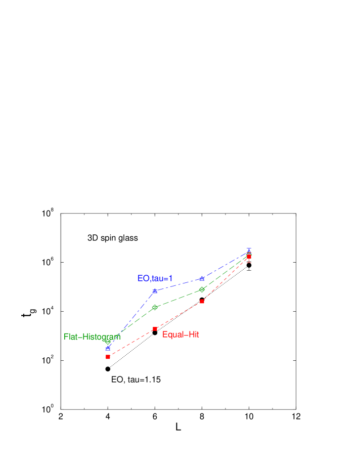
Figure 2: The average limiting time $t_{g}$ to find a ground state for the three-dimensional Ising spin-glass model. The meanings of the symbols are the same as those of Figure 1.

Another very interesting aspect of Fig. 1 is that the curves all look linear in the semi-logarithmic scale. This implies that $t_{g}\sim\exp(cL)$ for some constant $c\sim 1$, not a power law in $L$. Thus, all of the algorithms are asymptotically inefficient. It would be very interesting if this numerical observation can be supported by some argument. Similar results for the three-dimensional Ising spin glass is presented in Fig. 2.

$L=6$, MCS $=10^{6}$, sample $=1024$
	$t_{g}$	$E_{g}$
EO	$(6.95\pm 0.65)\times 10^{4}$	$-1.7713\pm 0.0012$
optimal EO	$(1.36\pm 0.15)\times 10^{3}$	$-1.7715\pm 0.0006$
Flat-Histogram	$(1.46\pm 0.13)\times 10^{4}$	$-1.7715\pm 0.0006$
Equal-Hit	$(1.92\pm 0.20)\times 10^{3}$	$-1.7716\pm 0.0006$
$L=10$, MCS $=10^{6}$, sample $=256$
	$t_{g}$	$E_{g}$
EO	$(2.98\pm 0.17)\times 10^{5}$	$-1.7721\pm 0.0008$
optimal EO	$(1.04\pm 0.11)\times 10^{5}$	$-1.7809\pm 0.0008$
Flat-Histogram	$(1.93\pm 0.15)\times 10^{5}$	$-1.7802\pm 0.0007$
Equal-Hit	$(1.27\pm 0.17)\times 10^{5}$	$-1.7815\pm 0.0010$

Table 1: The average time $t_{g}$ and lowest energy $E_{g}$ obtained for three-dimensional Ising spin-glass.

In Table 1, we report some typical data for the average first-passage time $t_{g}$, energy per site, length of the run, and number of random samples for four algorithms for the three-dimensional spin glasses. Since we use the same set of samples with the four algorithms, a lower energy indicates a better performance. The data show that equal-hit is comparable to EO at optimal $\tau$.

4 Turning EO into an equilibrium algorithm

The flat-histogram and equal-hit algorithms can be used for equilibrium simulation. With the help of counting the number of potential moves, $N_{k}$, a basic requirement for obtaining equilibrium property of the simulated model is the microcanonical property. Using the broad histogram equation [27, 28],

$$n(E)\langle N_{k}(\sigma)\rangle_{E}=n(E^{\prime})\langle N_{Z-k}(\sigma^{\prime})\rangle_{E^{\prime}},\qquad k=\bigl{(}(E^{\prime}-E)/J+2Z\bigr{)}/4,$$ (13)

we can obtain the density of states $n(E)$ of energy $E$, thus the equilibrium thermodynamic quantities, including free energy.

Unfortunately, the microcanonical property that the probability distribution $P(\sigma)$ of the configurations is a function of energy $E$ only is strongly violated in EO. The probabilities of the ground states cluster into groups, rather than uniformly distributed. Numerical tests show that $P(\sigma)$ is a function of $E$, $N_{k}$, as well as additional unknown parameters. To correct this problem, we introduce a rejection step in the EO algorithm, as follows:

$$W(\sigma\to\sigma^{\prime})=\delta_{N}(\sigma,\sigma^{\prime})P_{k}{1\over N_{k}}a(\sigma\to\sigma^{\prime}).$$ (14)

The acceptance rate $a$ is determined by imposing a detailed balance with an unknown probability distribution $f\bigl{(}E(\sigma)\bigr{)}$,

$$f\bigl{(}E(\sigma)\bigr{)}W(\sigma\to\sigma^{\prime})=f\bigl{(}E(\sigma^{\prime})\bigr{)}W(\sigma^{\prime}\to\sigma).$$ (15)

This gives an equation for the rate $a$:

$$f(E)P_{k}{1\over N_{k}(\sigma)}a(\sigma\to\sigma^{\prime})=f(E^{\prime})P^{\prime}_{Z-k}{1\over N_{Z-k}(\sigma^{\prime})}a(\sigma^{\prime}\to\sigma).$$ (16)

The prime on $P^{\prime}$ indicates that it is a set of $P$ values calculated from the state $\sigma^{\prime}$. A solution to this equation is a Metropolis-type choice:

$$a(\sigma\to\sigma^{\prime})=\min\left(1,{f(E^{\prime})P^{\prime}_{Z-k}/N_{Z-k}(\sigma^{\prime})\over f(E)P_{k}/N_{k}(\sigma)}\right).$$ (17)

To implement this, we need a two-pass simulation. The first pass determines the function $f(E)$. The procedure is by no means unique. Here, we collect histogram of energy $H(E)$ as well as statistics for $\langle N_{k}\rangle_{E}$ from an incorrect simulate of the original EO. Then we determine an approximate density of states with the help of the broad histogram equation, Eq. (13). The function $f$ is computed from $f(E)=H(E)/n(E)$. The EO with rejection is implemented in the second pass. The above procedure should be applicable for any model and any optimization algorithms that has a ‘steady state’. If the microcanonical property is only slightly violated, it will give a correct equilibrium algorithm with $a$ nearly equal to 1. Thus, we hope to have a method that is efficient for optimization, and yet at the same time, give correct equilibrium statistics.

Indeed, with the above method the microcanonical property is restored. Due to the rejection step, the dynamics is slightly changed. A consequence is that the histogram in the second pass shifted towards high energy side, thus the efficiency of the original EO is lost.

5 Conclusion

From this study, we show that equal-hit algorithm is an excellent candidate for ground state search. At the same time, it also offers the possibility for equilibrium calculations, such as the computation of the ground state entropy. We also show how optimization algorithms like EO can be turned into equilibrium algorithms by introducing a rejection step. All the algorithms studied here give rather rapid increase of $t_{g}$ with sizes, thus it is important and challenging to find algorithms that reduce this growth. Perhaps, algorithms based on single-spin-flip have their fundamental limitations.

References

- [1] S. Kirkpatrick, C. D. Gelatt, and M. P. Vecchi, Science 220, 671 (1983).
- [2] J. Holland, Adaptation in Natural and Artificial Systems (University of Michigan Press, Ann Arbor, 1975).
- [3] N. Kawashima and M. Suzuki, J. Phys. A: Math. Gen. 25, 1055 (1992).
- [4] F.-M. Dittes, Phys. Rev. Lett. 76, 4651 (1996).
- [5] K. F. Pal, Physica A 223, 283 (1996).
- [6] A. K. Hartmann, Europhys. Lett. 40, 429 (1997).
- [7] K. Chen, Europhys. Lett. 43, 635 (1998).
- [8] B. A. Berg and W. Janke, Phys. Rev. Lett. 80, 4771 (1998).
- [9] J. Houdayer and O. C. Martin, Phys. Rev. Lett. 83, 1030 (1999).
- [10] J. Dall, and P. Sibani, Comp. Phys. Commun. 141, 260 (2001).
- [11] S. Boettcher and A. G. Percus, Artif. Intellig. 119, 275 (2000).
- [12] S. Boettcher and A. G. Percus, Phys. Rev. Lett. 86, 5211 (2001).
- [13] P. Bak, C. Tang, and K. Wiesenfeld, Phys. Rev. Lett. 59, 381 (1987).
- [14] B. A. Berg and T. Neuhaus, Phys. Rev. Lett. 68, 9 (1992).
- [15] B. Hesselbo and R. B. Stinchcombe, Phys. Rev. Lett. 74, 2151 (1995).
- [16] K. Hukushima and Y. Nemoto, J. Phys. Soc. Jpn. 65, 1604 (1996).
- [17] J.-S. Wang, Eur. Phys. J. B 8, 287 (1999).
- [18] Z. F. Zhan, L. W. Lee, and J.-S. Wang, Physica A 285, 239 (2000).
- [19] K. Binder and A. P. Young, Rev. Mod. Phys. 58, 801 (1986); M. Mezard, G. Parisi, and M. A. Virasoro, Spin Glass Theory and Beyond (World Scientific, Singapore, 1987).
- [20] F. Barahona, J. Phys. A 15, 3241 (1982).
- [21] P. M. C. de Oliveira, T. J. P. Penna, H. J. Herrmann, Braz. J. Phys. 26, 677 (1996).
- [22] B. A. Berg, Nature, 361, 708 (1993).
- [23] A. B. Bortz, M. H. Kalos, J. L. Lebowitz, J. Comput. Phys. 17, 10 (1975).
- [24] J.-S. Wang and R. H. Swendsen, J. Stat. Phys. 106, 245 (2002).
- [25] R. H. Swendsen, B. Diggs, J.-S. Wang, S.-T. Li, C. Genovese, J. B. Kadane, Int. J. Mod. Phys. C 10, 1563 (1999).
- [26] http interface of the spin glass server is at http://www.informatik.uni-koeln.de/ls_juenger/projects/sgs.html. We thank Thomas Lange for generating the samples used in the comparisons.
- [27] P. M. C. de Oliveira, Eur. Phys. J. B 6, 111 (1998); P. M. C. Oliveira, cond-mat/0204332.
- [28] B. A. Berg and U. H. E. Hansmann, Euro. Phys. J B 6, 395 (1998).