Theory of the Ramsey spectroscopy and anomalous segregation in ultra-cold rubidium

Abstract

The recent anomalous segregation experiment [1] shows dramatic, rapid internal state segregation for two hyperfine levels of $\phantom{|}{}^{87}{\rm Rb}$. We simulate an effective one dimensional model of the system for experimental parameters and find reasonable agreement with the data. The Ramsey frequency is found to be insensitive to the decoherence of the superposition, and is only equivalent to the interaction energy shift for a pure superposition. A Quantum Boltzmann equation describing collisions is derived using Quantum Kinetic Theory, taking into account the different scattering lengths of the internal states. As spin-wave experiments are likely to be attempted at lower temperatures we examine the effect of degeneracy on decoherence by considering the recent experiment [1] where degeneracy is around $10\%$. We also find that the segregation effect is only possible when transport terms are included in the equations of motion, and that the interactions only directly alter the momentum distributions of the states. The segregation or spin wave effect is thus entirely due to coherent atomic motion as foreseen in [1].

1 Introduction

A topic of great interest in many particle quantum mechanics is the effect of coherence in mesoscopic systems. The recent experiment at JILA [1] shows transient highly non-classical behaviour, characteristic of such phenomena. An ultra-cold non-condensed gas of $\phantom{|}{}^{87}{\rm Rb}$  is harmonically trapped and prepared in a superposition of two hyperfine states by a two photon $\pi/2$ pulse. The superposition is allowed to evolve for a range of different times and the densities of the two levels measured across the trap; the data are then collected via absorption imaging. In the cold collision regime of the experiment the two states interact via slightly different S-wave scattering lengths; moreover, the states experience different Zeeman shifts in the presence of a magnetic bias field, and the combination of these effects produces an effective potential between the two states [1]. This differential potential was characterized using the Ramsey spectroscopy technique, and the segregation effect was explored for different potentials and atom densities. When the differential potential is constant across the cloud the motion is not observed. When the differential potential has a gradient across the cloud the atoms appear to redistribute in the trap, as long as the two states are in a partial superposition. The dissipation of the coherent relationship between the states is responsible for the transience of the spin waves.

The original experiment [1] stimulated much work on this system. Three theoretical treatments [4, 3, 5] found good agreement between simulations of the segregation dynamics and the evolution of the experimentally measured distributions reported in [1]. These works all use the spin operator notation and treat the system as essentially a spin wave problem. More recently, detailed imaging of the Bloch vector was carried out during spin wave motion in [8]. Simulations of linearized spin kinetic equations also showed good agreement for the frequencies and damping damping times of linearized collective modes [9]. We do not use a spin operator formalism in this paper, although this has no effect on our results.

The outline of this paper is as follows. The equations of motion are found from the Hamiltonian for the system in Section 2. The spectroscopy of the initial state is outlined in Section 3. The interpretation of the Ramsey experiment and the interaction energy are discussed in Section 4. In Section 5 the issue of damping is addressed. A Quantum Boltzmann equation describing the effects of collisions on the distributions for states with different scattering lengths is derived, and we discuss the relaxation time approximations used in the simulations presented in Section 6. In Section 7 we consider the question posed in the experimental report regarding the physical state of motion of the atoms during the segregation.

2 Theoretical Framework

2.1 Second Quantized Hamiltonian

The second quantized Hamiltonian for a coherently coupled two state gas is

$$H = \int d^{3}{\bf x}\,\Bigg{\{}\psi^{\dagger}_{1}H_{1}({\bf x})\psi_{1}+\psi^{\dagger}_{2}H_{1}({\bf x})\psi_{2}$$ (1)

$$+{u_{11}\over 2}\psi^{\dagger}_{1}\psi^{\dagger}_{1}\psi_{1}\psi_{1}+{u_{12}}\psi^{\dagger}_{1}\psi^{\dagger}_{2}\psi_{1}\psi_{2}+{u_{22}\over 2}\psi^{\dagger}_{2}\psi^{\dagger}_{2}\psi_{2}\psi_{2}$$

$$+gE({\bf x})\bigg{(}\psi^{\dagger}_{1}\psi_{2}e^{i\Omega t}+\psi^{\dagger}_{2}\psi_{1}e^{-i\Omega t}\bigg{)}\Bigg{\}},$$

where

$$H_{j}({\bf x})=-{\hbar^{2}\nabla^{2}\over 2m}+V_{j}({\bf x})+\hbar\omega_{j}({\bf x})$$ (2)

for $j=1,2$, and $g$ is only nonzero during the initial two photon pulse, creating a coherent superposition of the two hyperfine states. Note that the Zeeman splitting of the transition frequency is position dependent but this is absorbed into the effective external potentials. The Heisenberg equations of motion for the field operators are

$$i\hbar\dot{\psi}_{1} = H_{1}({\bf x})\psi_{1}+u_{11}\psi^{{\dagger}}_{1}\psi_{1}\psi_{1}+u_{12}\psi^{\dagger}_{2}\psi_{2}\psi_{1}+gE({\bf x})\psi_{2}e^{i\Omega t},$$ (3)

$$i\hbar\dot{\psi}_{2} = H_{2}({\bf x})\psi_{2}+u_{22}\psi_{2}^{\dagger}\psi_{2}\psi_{2}+u_{12}\psi^{\dagger}_{1}\psi_{1}\psi_{2}+gE({\bf x})\psi_{1}e^{-i\Omega t}.$$ (4)

2.2 Experimental Details

The experiment uses an ultra cold non-condensed $\phantom{|}{}^{87}{\rm Rb}$  gas held in a harmonic trap at temperatures T$\sim 850\;$nK. The trap is a cigar shape with frequencies $\omega_{r}=2\pi\times 7\;$Hz and $\omega_{z}=2\pi\times 230\;$Hz. A $\pi/2$ two photon pulse is used to create a superposition of the $|1\rangle\equiv|F=1,m_{F}=-1\rangle$ and $|2\rangle\equiv|F=2,m_{F}=1\rangle$ hyperfine states from a thermal equilibrium $|1\rangle$ gas. The s-wave scattering lengths between the hyperfine states $|i\rangle$ and $|j\rangle$, $a_{ij}$, are $a_{11}=100.9a_{0}$, $a_{12}=98.2a_{0}$ and $a_{22}=95.6a_{0}$, where $a_{0}$ is the Bohr radius[1]. In the usual cold collision pseudo-potential approximation this leads to the interaction strengths

$$u_{ij}=4\pi\hbar^{2}a_{ij}/m_{R}.$$ (5)

where $m$ is the $\phantom{|}{}^{87}{\rm Rb}$  mass. Since the scattering lengths are so similar, and almost evenly split about $a_{12}$ we define the interaction splitting

$$\delta u \equiv u_{11}-u_{22}=5.3{4\pi\hbar^{2}a_{0}\over m},$$ (6)

and use the approximations

$$u_{11}-u_{12} = 2.7{4\pi\hbar^{2}a_{0}\over m}\simeq\delta u/2,$$ (7)

$$u_{12}-u_{22} = 2.6{4\pi\hbar^{2}a_{0}\over m}\simeq\delta u/2,$$ (8)

in the remainder of this paper.

A magnetic bias field is used to change the effective differential force exerted on the two states, and can be chosen to either cancel or enhance the mean field force. Segregation of the two species is observed via a subsequent two photon pulse which causes a transition to an internal state appropriate for absorption imaging. The magnetic bias field is used to control the onset of segregation for a given density, or alternatively the density may be increased for a fixed bias strength to produce a similar effect.

2.3 Equations of Motion

In order to simulate the full behaviour of this system we wish to find suitable equations of motion to describe the system in the Hartree-Fock regime, where a local density approximation is valid. Defining the Wigner amplitudes

$$n_{j}({\bf x},{\bf p})=\int d^{3}{\bf y}\langle\psi^{\dagger}_{j}({\bf x}-{\bf y}/2)\psi_{j}({\bf x}+{\bf y}/2)\rangle e^{-i{\bf p}\cdot{\bf y}/\hbar},$$ (9)

$$f({\bf x},{\bf p})=\int d^{3}{\bf y}\langle\psi^{\dagger}_{1}({\bf x}-{\bf y}/2)\psi_{2}({\bf x}+{\bf y}/2)\rangle e^{-i{\bf p}\cdot{\bf y}/\hbar},$$ (10)

so that the densities are

$$N_{j}({\bf x})=\int{d^{3}{\bf p}\over(2\pi\hbar)^{3}}\;n_{j}({\bf x},{\bf p})\equiv\langle\psi^{\dagger}_{j}({\bf x})\psi_{j}({\bf x})\rangle,$$ (11)

$$F({\bf x})=\int{d^{3}{\bf p}\over(2\pi\hbar)^{3}}\;f({\bf x},{\bf p})\equiv\langle\psi^{\dagger}_{1}({\bf x})\psi_{2}({\bf x})\rangle,$$ (12)

and using Hartree-Fock factorisation and standard Wigner function methods [2], the equations of motion are written in terms of $n({\bf x},{\bf p})\equiv n_{1}({\bf x},{\bf p})+n_{2}({\bf x},{\bf p})$ and the segregation $m({\bf x},{\bf p})\equiv n_{1}({\bf x},{\bf p})-n_{2}({\bf x},{\bf p})$ as

$$\dot{n}({\bf x},{\bf p}) = \left\{-({\bf p}/m)\cdot\nabla_{\bf x}+\nabla V_{\rm eff}({\bf x})\cdot\nabla_{\bf p}\right\}n({\bf x},{\bf p})$$ (13)

$$-{1\over 2}\nabla V_{\rm diff}({\bf x})\cdot\nabla_{\bf p}m({\bf x},{\bf p})$$

$$+u_{12}\big{\{}\nabla F({\bf x})\cdot\nabla_{\bf p}f({\bf x},{\bf p})^{*}+\nabla F({\bf x})^{*}\cdot\nabla_{\bf p}f({\bf x},{\bf p})\big{\}},$$

$$\dot{m}({\bf x},{\bf p}) = \left\{-({\bf p}/m)\cdot\nabla_{\bf x}+\nabla V_{\rm eff}({\bf x})\cdot\nabla_{\bf p}\right\}m({\bf x},{\bf p})$$ (14)

$$-{1\over 2}\nabla V_{\rm diff}({\bf x})\cdot\nabla_{\bf p}n({\bf x},{\bf p})$$

$$-{2iu_{12}\over\hbar}\big{\{}f({\bf x},{\bf p})F({\bf x})^{*}-f({\bf x},{\bf p})^{*}F({\bf x})\big{\}},$$

$$\dot{f}({\bf x},{\bf p}) = \left\{-({\bf p}/m)\cdot\nabla_{\bf x}+\nabla V_{\rm eff}({\bf x})\cdot\nabla_{\bf p}\right\}f({\bf x},{\bf p})$$ (15)

$$-i{V_{\rm diff}({\bf x})\over\hbar}f({\bf x},{\bf p})$$

$$-i{u_{12}\over\hbar}\left(m({\bf x},{\bf p})F({\bf x})-f({\bf x},{\bf p})M({\bf x})\right)$$

$$+{u_{12}\over 2}\nabla F({\bf x})\cdot\nabla_{\bf p}n({\bf x},{\bf p}),$$

where the potentials are

$$V_{\rm eff}({\bf x}) = {1\over 2}\bigg{(}V_{1}({\bf x})+V_{2}({\bf x})+3u_{12}N({\bf x})+\delta u\;M({\bf x})\bigg{)},$$ (16)

$$V_{\rm diff}({\bf x}) = \hbar\Delta\omega_{\rm z}({\bf x})+\hbar\Delta\omega_{\rm c}({\bf x}).$$ (17)

and the frequencies are the coherent frequency shift

$$\hbar\Delta\omega_{\rm c}({\bf x}) \equiv 2u_{22}N_{2}({\bf x})-2u_{11}N_{1}({\bf x})+2u_{12}(N_{1}({\bf x})-N_{2}({\bf x}))$$ (18)

$$\simeq -\delta uN({\bf x}),$$

and the Zeeman shift

$$\hbar\Delta\omega_{\rm z}({\bf x}) \equiv \hbar\left(\omega_{2}({\bf x})-\omega_{1}({\bf x})\right)=V_{2}({\bf x})-V_{1}({\bf x}).$$ (19)

For the low densities employed these equations of motion are nearly exact for the thermal gas, apart from the relaxation caused by collisions.

3 Spectroscopy of the initial state

The result of the laser excitation is to rotate the spin wavefunction into the $|2\rangle$ subspace, so the one-body wavefunction is transformed to

$$|1{\bf}\rangle\to t|1{\bf}\rangle+r|2{\bf}\rangle,$$ (20)

with $|t|^{2}+|r|^{2}=1$. In field theoretic language (in the Heisenberg picture) we describe the initial state by the field operators $\psi_{i1}({\bf x})$ and $\psi_{i2}({\bf x})$, where the subscript $i$ denotes refers to the initial state before the pulse. These transform to

$$\psi_{i1}({\bf x}) \to \psi_{1}({\bf x})=\phantom{-}t\psi_{i1}({\bf x})+r\psi_{i2}({\bf x})$$ (21)

$$\psi_{i2}({\bf x}) \to \psi_{2}({\bf x})=-r\psi_{i1}({\bf x})+t\psi_{i2}({\bf x}),$$ (22)

where the condition $|t|^{2}+|r|^{2}=1$ ensures the conservation of total number and $r$ and $t$ are chosen real. We denote the population densities by $N_{j}({\bf x})=\langle\psi^{\dagger}_{j}({\bf x})\psi_{j}({\bf x})\rangle$, and the coherence amplitude by $F({\bf x})=\langle\psi^{\dagger}_{1}({\bf x})\psi_{2}({\bf x})\rangle$. In general the population densities transform to

$$N_{i1}({\bf x})\to N_{1}({\bf x}) = |t|^{2}N_{i1}({\bf x})+|r|^{2}N_{i2}({\bf x})+t^{*}rF_{i}({\bf x})+r^{*}tF_{i}^{*}({\bf x}),$$ (23)

$$N_{i2}({\bf x})\to N_{2}({\bf x}) = |r|^{2}N_{i1}({\bf x})+|t|^{2}N_{i2}({\bf x})-t^{*}rF_{i}^{*}({\bf x})-r^{*}tF_{i}({\bf x}),$$ (24)

For the $\phantom{|}{}^{87}{\rm Rb}$  experiment the initial occupation of the 2 state is zero, so that $N_{i1}({\bf x})=N({\bf x})$, $N_{i2}({\bf x})=F_{i}({\bf x})=0$ and a two photon pulse causes the transformation

$$N_{i1}({\bf x}) \to N_{1}({\bf x})=\phantom{-}|t|^{2}N({\bf x}),$$ (25)

$$N_{i2}({\bf x}) \to N_{2}({\bf x})=\phantom{-}|r|^{2}N({\bf x}),$$ (26)

$$\phantom{-}F_{i}({\bf x}) \to \phantom{2}F({\bf x})=-t^{*}rN({\bf x}),$$ (27)

$$|F_{i}({\bf x})|^{2} \to |F({\bf x})|^{2}=N_{1}({\bf x})N_{2}({\bf x}),$$ (28)

so that (28) corresponds to a fully coherent superposition.

3.1 Energy Density

If we consider the total energy density we have in general

$$U({\bf x}) \equiv \left\langle\psi_{1}\left(-{\hbar^{2}\nabla^{2}\over 2m}+V_{1}({\bf x})\right)\psi_{1}\right\rangle+\left\langle\psi_{2}\left(-{\hbar^{2}\nabla^{2}\over 2m}+V_{2}({\bf x})\right)\psi_{2}\right\rangle$$ (29)

$$+\left\langle{u_{11}\over 2}\psi^{\dagger}_{1}\psi^{\dagger}_{1}\psi_{1}\psi_{1}+{u_{12}}\psi^{\dagger}_{1}\psi^{\dagger}_{2}\psi_{1}\psi_{2}+{u_{22}\over 2}\psi^{\dagger}_{2}\psi^{\dagger}_{2}\psi_{2}\psi_{2}\right\rangle.$$

Changing the internal state of an atom does not change its velocity so the kinetic energy terms may be ignored in finding the change in energy of the gas during the transition. Using Hartree-Fock factorization and (25-28), the energy density is

$$U({\bf x}) = u_{11}N_{1}({\bf x})^{2}+u_{12}(|F({\bf x})|^{2}+N_{1}({\bf x})N_{2}({\bf x}))+u_{22}N_{2}({\bf x})^{2}$$ (30)

$$+V_{1}({\bf x})N_{1}({\bf x})+V_{2}({\bf x})N_{2}({\bf x}).$$

Evaluating the change in energy density for an arbitrary rotation defined by (21), (22) leads to

$$\Delta U({\bf x}) = \bigg{(}u_{11}(|t|^{4}-1)+2u_{12}|t|^{2}|r|^{2}+u_{22}|r|^{4}\bigg{)}N({\bf x})^{2}$$ (31)

$$+(V_{2}-V_{1})|r|^{2}N({\bf x}).$$

3.1.1 Infinitesimal rotation

For a very small rotation $|r|^{2}\ll 1$ and $1-|t|^{4}\simeq 2|r|^{2}$. Putting $N_{2}({\bf x})=\delta N({\bf x})\ll N({\bf x})$, $|r|^{4}\simeq 0$ and $N_{1}({\bf x})\simeq N({\bf x})$, we find

$$\Delta U({\bf x}) = \delta N({\bf x})\bigg{(}2(u_{12}-u_{11})N({\bf x})+V_{2}({\bf x})-V_{1}({\bf x})\bigg{)},$$ (32)

For $\phantom{|}{}^{87}{\rm Rb}$  this becomes (using (7, 8))

$$\Delta U({\bf x}) = \delta N({\bf x})\bigg{(}-\delta u\;N({\bf x})+V_{2}({\bf x})-V_{1}({\bf x})\bigg{)}=\delta N({\bf x})V_{\rm diff}({\bf x}),$$ (33)

so that the change in energy density varies linearly with the number of atoms transferred to the higher energy state, and is proportional to the differential potential.

3.1.2 $\pi/2$ pulse

For a $\pi/2$ pulse the energy density change is

$$\Delta U({\bf x}) = \bigg{(}3u_{11}+2u_{12}+u_{22}\bigg{)}{N({\bf x})^{2}\over 4}+(V_{2}({\bf x})-V_{1}({\bf x})){N({\bf x})\over 2}.$$ (34)

For $\phantom{|}{}^{87}{\rm Rb}$  this becomes

$$\Delta U({\bf x}) = \bigg{(}3u_{12}+\delta u\bigg{)}{N({\bf x})^{2}\over 2}+(V_{2}({\bf x})-V_{1}({\bf x})){N({\bf x})\over 2}.$$ (35)

Thus the effect of an intense pulse is to produce a nonlinear change in the energy density via the mean field interactions.

3.2 Coherence energy

The analysis is simplified by noting that because the only net force in the experiment is a weak differential force between the two internal states, the total atomic density is approximately conserved. The experimental data suggests that this is a reasonable approximation [1], and our detailed simulations confirm this expectation. Treating $N(\bf{x})$ as constant allows insight into the energy conserving processes in the dynamics. In terms of the normalized moments $\langle{\bf p}_{j}^{k}({\bf x})\rangle=\int d^{3}{\bf p}\;{\bf p}^{k}n_{j}({\bf x},{\bf p})/N_{j}({\bf x})(2\pi\hbar)^{3}$ we have the relations

$$N_{1}({\bf x})\langle{\bf p}_{1}({\bf x})\rangle+N_{2}({\bf x})\langle{\bf p}_{2}({\bf x})\rangle=N({\bf x})\langle{\bf p}({\bf x})\rangle=0$$ (36)

(which is essentially momentum conservation in the absence of any external perturbation of the stationary density profile), and for the total kinetic energy density

$${N_{1}({\bf x})\langle{\bf p}_{1}^{2}({\bf x})\rangle\over 2m}+{N_{2}({\bf x})\langle{\bf p}_{2}^{2}({\bf x})\rangle\over 2m}={N({\bf x})\langle{\bf p}^{2}({\bf x})\rangle\over 2m}.$$ (37)

Here only $N({\bf x})$ is constant since the other moments and densities will change during the relative motion of the two species. We may now write (30) in the form

$$U({\bf x}) = {3u_{12}\over 4}N({\bf x})^{2}+{\left(V_{1}({\bf x})+V_{2}({\bf x})\right)\over 2}N({\bf x})$$ (41)

$$+{u_{12}\over 4}M({\bf x})^{2}+{\delta u\over 2}N({\bf x})M({\bf x})-{1\over 2}\hbar\Delta\omega_{\rm z}({\bf x})M({\bf x})$$

$$+u_{12}|F({\bf x})|^{2}$$

$$+N({\bf x}){\langle{\bf p}^{2}({\bf x})\rangle\over 2m},$$

where the spatial segregation is $M({\bf x})\equiv\int\;d^{3}{\bf p}\;m({\bf x},{\bf p})/(2\pi\hbar)^{3}$. The first line is constant in time, and the second line only varies with $M({\bf x})$. The third line is the coherence energy density which may change during the motion, while the last line is a function of the local densities and temperatures through (37). It is clear that the coherence energy moves between $F({\bf x})$ and $M({\bf x})$ via relative motion which changes the local temperature and momentum of each distribution.

4 The Ramsey frequency and the interaction energy shift

The Ramsey technique has recently been shown to be a particularly useful tool for exploring the coherence properties of ultracold dilute gases [1, 11, 8]. In applying the technique to the ultra-cold non-condensed gases of these experiments there remains an issue in the interpretation of the technique which we wish to resolve. The problem is whether or not the Ramsey frequency is sensitive to the decoherence of the superposition of internal states required to resolve the Ramsey fringes. The Ramsey technique has been developed and used extensively for probing the relative energies of internal states in non-interacting atomic beams. When interactions are negligible the measured quantity is the energy difference between the two internal states of the superposition. We will see that for the interacting case, this is only partially true because interactions produce a transient mean field energy which decays with the coherence of the superposition.

4.1 Experiment

The experiment measures the frequency of oscillation for the relative occupation of the two internal states, after a second $\pi/2$ pulse is applied to the system. The final two photon pulse transforms the fields to

$$\psi_{1}\rightarrow{\psi_{1}+\psi_{2}\over\sqrt{2}},$$ (42)

$$\psi_{2}\rightarrow{\psi_{2}-\psi_{1}\over\sqrt{2}}.$$ (43)

In terms of the densities $N_{i}({\bf x})\equiv\langle\psi^{\dagger}_{i}\psi_{i}\rangle$, and the coherence amplitude $F({\bf x})\equiv\langle\psi_{1}^{\dagger}\psi_{2}\rangle$, the ratio of the densities may be written

$${N_{2}({\bf x})\over N_{1}({\bf x})}={N({\bf x})-2{\rm Re\;}F({\bf x})\over N({\bf x})+2{\rm Re\;}F({\bf x})},$$ (44)

where $N({\bf x})=N_{1}({\bf x})+N_{2}({\bf x})$ may be assumed invariant. The ratio will then only depend on $F({\bf x})$; in particular, it will oscillate at the same frequency. Applying the second $\pi/2$ pulse at different times and measuring $N_{1}({\bf x})/N_{2}({\bf x})$ thus determines the frequency of $F({\bf x})$, and this is the frequency accessible via the Ramsey technique of [1, 8].

4.2 Coherence equation

In a typical experiment [1, 8], a $\pi/2$ pulse generates an equal superposition of the two hyperfine states which is then allowed to evolve without coupling until a second $\pi/2$ pulse is applied. We are primarily interested in the influence of the interactions on the Ramsey frequency, and after the first pulse the Heisenberg equations of motion generated by the interaction terms in the Hamiltonian (1) are

$$i\hbar\dot{\psi}_{1} = u_{11}\psi^{{\dagger}}_{1}\psi_{1}\psi_{1}+u_{12}\psi^{\dagger}_{2}\psi_{2}\psi_{1},$$ (45)

$$i\hbar\dot{\psi}_{2} = u_{22}\psi_{2}^{\dagger}\psi_{2}\psi_{2}+u_{12}\psi^{\dagger}_{1}\psi_{1}\psi_{2}.$$ (46)

The operators $\psi_{1}^{\dagger}\psi_{1}$ and $\psi_{2}^{\dagger}\psi_{2}$ commute with the Hamiltonian when $E({\bf x})=0$, so the occupations are preserved. The equation of motion for the coherence is

$$i\hbar{d\langle\psi_{1}^{\dagger}\psi_{2}\rangle\over dt} = u_{22}\langle\psi_{1}^{\dagger}\psi_{2}^{\dagger}\psi_{2}\psi_{2}\rangle+u_{12}\langle\psi_{1}^{\dagger}\psi_{1}^{\dagger}\psi_{1}\psi_{2}\rangle$$ (47)

$$- u_{11}\langle\psi_{1}^{\dagger}\psi_{1}^{\dagger}\psi_{1}\psi_{2}\rangle-u_{12}\langle\psi_{1}^{\dagger}\psi_{2}^{\dagger}\psi_{2}\psi_{2}\rangle.$$

4.3 Four point averages

There are two equivalent ways of treating the four point averages when the system is noncondensed and thermal, both of which lead to results of the form

$$\langle\psi_{1}^{\dagger}\psi_{1}^{\dagger}\psi_{1}\psi_{2}\rangle = 2N_{1}({\bf x})F({\bf x}).$$ (48)

• When the initial quantum state is nondegenerate, each field may be written in terms of a set of orthonormal single particle wavefunctions $\phi_{r}({\bf x})$

  $$\psi_{i}=\sum_{r}\phi_{r}({\bf x})a_{ir},$$ (49)

  where $[a_{ir},a_{jk}^{\dagger}]=\delta_{ij}\delta_{rk}$. The densities and coherence then read

  $$\langle\psi^{\dagger}_{i}\psi_{j}\rangle=\sum_{r,s}\phi_{r}({\bf x})^{*}\phi_{s}({\bf x})\langle a^{\dagger}_{ir}a_{js}\rangle.$$ (50)

  The eigenvalues of the operators $N_{ir}=a_{ir}^{\dagger}a_{ir}$ which contribute significantly are either 0 or 1. We can describe the situation by the averages

  $$\langle a_{ir}^{\dagger}a_{ir}\rangle \equiv \bar{N}_{ir},$$ (51)

  $$\langle a_{1r}^{\dagger}a_{2r}\rangle \equiv \bar{M}_{r}.$$ (52)

  For all averages $\langle a_{ir}^{\dagger}a_{js}\rangle=0$ when $r\neq s$, corresponding to independently occupied modes. We then have

  $$\langle\psi_{1}^{\dagger}\psi_{2}\rangle=\sum_{r}|\phi_{r}({\bf x})|^{2}\bar{M}_{r},$$ (53)

  and the four point averages become, for example

  $$\langle a_{1r}^{\dagger}a_{1s}^{\dagger}a_{1j}a_{2k}\rangle = \cases{&\hskip-17.07164pt$\delta_{rj}\delta_{sk}\bar{N}_{1r}\bar{M}_{s}+\delta_{sj}\delta_{rk}\bar{N}_{1s}\bar{M}_{r}$\;\;when $r\neq s$ and $j\neq k$,\\ &\hskip-17.07164pt0\;\;otherwise.\\ }$$ (54)

  The four point average becomes

  $$\langle\psi_{1}^{\dagger}\psi_{1}^{\dagger}\psi_{1}\psi_{2}\rangle = 2\sum_{r,s,\;r\neq s}|\phi_{r}({\bf x})|^{2}|\phi_{s}({\bf x})|^{2}\bar{N}_{1r}\bar{M}_{s},$$ (55)

  $$\simeq 2N_{1}({\bf x})F({\bf x}),$$

  where the approximation is valid if the occupation is spread over very many modes, as for a thermal state, so that the term with $r=s$ is negligible.

• Alternatively, the same result may be found using Hartree-Fock factorization for the averages over the field operators. This method uses the Gaussian statistics of the thermal gas, which may hold under more general circumstances than the arguments of i), but is equivalent for the system under consideration. The averages are

  $$\langle\psi_{1}^{\dagger}\psi_{2}^{\dagger}\psi_{3}\psi_{4}\rangle=\langle\psi_{1}^{\dagger}\psi_{3}\rangle\langle\psi_{2}^{\dagger}\psi_{4}\rangle+\langle\psi_{1}^{\dagger}\psi_{4}\rangle\langle\psi_{2}^{\dagger}\psi_{3}\rangle+\langle\psi_{1}^{\dagger}\psi_{2}^{\dagger}\rangle\langle\psi_{3}\psi_{4}\rangle.$$ (56)

  For a thermal gas there is no anomalous average, so we recover the same result as (55)

  $$\langle\psi_{1}^{\dagger}\psi_{1}^{\dagger}\psi_{1}\psi_{2}\rangle=2N_{1}({\bf x})F({\bf x}).$$ (57)

4.4 Ramsey frequency

Using either approach, the equation of motion for the coherence becomes

$$i\hbar{d\over dt}F({\bf x}) = \left[2u_{22}N_{2}({\bf x})-2u_{11}N_{1}({\bf x})+2u_{12}(N_{1}({\bf x})-N_{2}({\bf x}))\right]F({\bf x})$$ (58)

$$\equiv \hbar\omega_{R}({\bf x})F({\bf x}).$$

Thus if the gas is thermal, the frequency of oscillation $\omega_{R}({\bf x})$ is independent of the amplitude $|F({\bf x})|$. In particular if some kind of damping reduces $|F({\bf x})|$ with time, this does not change the Ramsey frequency.

4.4.1 Transport and trap effects

The full equation of motion (15) may be integrated to find

$${\partial F({\bf x})\over\partial t}+\nabla\cdot(F({\bf x}){\bf v}_{F}({\bf x})) = -i\left(\Delta\omega_{c}({\bf x})+\Delta\omega_{\rm z}({\bf x})\right)F({\bf x})$$ (59)

$$\equiv -i\omega_{R}({\bf x})F({\bf x})$$

where the velocity is

$${\bf v}_{F}({\bf x})={1\over mF({\bf x})}\int{d^{3}{\bf p}\over(2\pi\hbar)^{3}}{\bf p}f({\bf x},{\bf p}).$$ (60)

When the velocity vanishes we recover (58) with an additional shift caused by the trap energy difference for the two states. The coherence current described by ${\bf v}_{F}$ may alter the measured Ramsey fringes, and indeed full simulations may be required for comparison with experiment when significant motion occurs.

4.5 Interaction energy shift

The quantity which is sensitive to the loss of coherence is the interaction energy, which in general does not correspond to the Ramsey frequency $\omega_{R}({\bf x})$.

The interaction energy change caused by changing the internal state from $|1\rangle$ to $|2\rangle$ is found from the chemical potentials associated with this change

$$\mu_{j}({\bf x}) \equiv {\partial U({\bf x})\over\partial N_{j}({\bf x})}.$$ (61)

Neglecting the transport and trap terms for simplicity, we use the mean energy density for the interactions

$$U({\bf x})={u_{11}\over 2}\langle\psi_{1}^{\dagger}\psi_{1}^{\dagger}\psi_{1}\psi_{1}\rangle+u_{12}\langle\psi_{1}^{\dagger}\psi_{2}^{\dagger}\psi_{1}\psi_{2}\rangle+{u_{22}\over 2}\langle\psi_{2}^{\dagger}\psi_{2}^{\dagger}\psi_{2}\psi_{2}\rangle,$$ (62)

and factorize averages as in (55), to find

$$\mu_{1} = 2u_{11}N_{1}+u_{12}N_{2}+{\partial|F|^{2}\over\partial N_{1}},$$ (63)

$$\mu_{2} = 2u_{22}N_{2}+u_{12}N_{1}+{\partial|F|^{2}\over\partial N_{2}}.$$ (64)

The change in energy caused by this transition is $\Delta\mu=\mu_{2}-\mu_{1}\equiv\hbar\Delta\omega_{\mu}$, so that using (63), (64) we find

$$\hbar\Delta\omega_{\mu} = 2u_{22}N_{2}-2u_{11}N_{1}+u_{12}(N_{1}-N_{2})$$ (65)

$$+u_{12}{\partial|F|^{2}\over\partial N_{2}}-u_{12}{\partial|F|^{2}\over\partial N_{1}}.$$

The derivatives of the coherence energy density are not evaluated because it is not usually possible to do so in any direct manner since $|F({\bf x})|^{2}$ cannot generally be specified by knowledge of the $N_{i}({\bf x})$. The Cauchy-Schwartz inequality leads to

$$|F({\bf x})|^{2}\leq N_{1}({\bf x})N_{2}({\bf x}).$$ (66)

When $|F({\bf x})|^{2}=N_{1}({\bf x})N_{2}({\bf x})$ the superposition is purely coherent, leading to a factor of 2 in the cross interaction part of the frequency shift; whereas for $|F|^{2}=0$ the extra factor due to the coherence is absent and we recover the thermal result. A simple model which we will use is found by taking $|F|^{2}=\alpha(t)N_{1}N_{2}$, with $\alpha(0)=1$ reconstructing the initial condition (28), and $\alpha(t\to\infty)=0$ medelling the damping to thermal equilibrium. The mean field energy shift becomes

$$\hbar\Delta\omega_{\mu}=2u_{22}N_{2}-2u_{11}N_{1}+2\alpha(t)u_{12}(N_{1}-N_{2})$$ (67)

Immediately after the pulse

$$\Delta\omega_{\mu}({\bf x})=\omega_{R}({\bf x}),$$ (68)

so that for short times the Ramsey frequency coincides with the interaction energy shift. Inclusion of the effect of collisions will cause $|F({\bf x})|$ to decay with time. The simplest way of doing this is to consider the case where there is no differential potential gradient so that segregation cannot occur. The collisions will still have a relaxation effect on the coherence and as a first approximation we may use the equation of motion

$$\dot{F}=-i\omega_{R}({\bf x})F-{1\over\tau_{c}}F,$$ (69)

where $\tau_{c}$ is the timescale of relaxation. Solving this and using (65) gives

$$\hbar\Delta\omega_{\mu}=2u_{22}N_{2}-2u_{11}N_{1}+u_{12}(N_{1}-N_{2})(1+\rme^{-2t/\tau_{c}}).$$

Clearly the mean field energy shift is sensitive to the decay of coherence, and decays at twice the rate for the amplitude.

5 Kinetic Theory of Coherence Damping

We now consider the role of collisions in dissipating coherence. Our starting point is the quantum kinetic theory of Gardiner and Zoller [7], which may be used to find an expression for the damping rate of $f({\bf x},{\bf p})$. While the expressions found are quite explicit, they are not easy to simulate, so that for the actual simulations we will use simplified forms based on a relaxation time approximation.

5.1 Quantum Kinetic Theory with internal degrees of freedom

In order to derive the damping for $f({\bf x},{\bf p})$ we first consider the damping term in the equation of motion for the reduced density matrix for a gas with a single internal state. For brevity of notation we suppress ${\bf x}$ arguments where possible since the damping is local. For ease of comparison with [7] we carry out the following in ${\bf K}$ variables. We seek the equation of motion for the terms

$$f_{lm}({\bf x},{\bf k})=\int d^{3}{\bf y}\langle\psi_{l}^{\dagger}({\bf x}-{\bf y}/2)\psi_{m}({\bf x}+{\bf y}/2)\rangle\rme^{-i{\bf k}\cdot{\bf y}}$$ (71)

where $l,m=1,2$. The derivation of the Quantum Boltzmann equation may then be carried out along similar lines to that in [7]. The principal modification of the derivation is due to the different scattering allowed between distinguishable internal states of the particles, and the preservation of possible coherence between internal states. The resolution of the field operator for internal state $i$ into its momentum components $\psi_{i{\bf K}}({\bf x})$ is defined similarly to (31) of [7] as

$$\psi_{i}({\bf x})=\sum_{{\bf K}}\rme^{-i{\bf K}\cdot{\bf x}}\psi_{i{\bf K}}({\bf x}).$$ (72)

The projector defined in (48) of [7] for the derivation of the master equation simplifies slightly because no Bose-Einstein condensate is present in this case, and becomes

$$p_{{\bf N}}|{\bf n}\rangle=\cases{&$|{\bf n}\rangle$\;\;if\;\; $\sum_{{\bf r},i}n_{i}({\bf K},{\bf r})=N({\bf K})$\\ &$0$\;\; otherwise.\\ }$$ (73)

This projector identifies all configurations with the same distribution in ${\bf K}$, but leaves the position and internal state distributions undisturbed. To evaluate the effect of collisions on the coherence we require the equation of motion for the reduced density matrix

$${\cal P}_{{\bf N}}\rho=p_{{\bf N}}\rho p_{{\bf N}}\equiv v_{{\bf N}},$$ (74)

induced by the interaction Hamiltonian

$$H_{I}={1\over 2}\sum_{ij,\;{\bf e}}U_{ij}(1,2,3,4),$$ (75)

in which we have used the notation for the sum over all momenta defined in [7]

$$\sum_{\bf e}\equiv\sum_{{\bf K}_{1},{\bf K}_{2},{\bf K}_{3},{\bf K}_{4}},$$ (76)

and the interaction operator $U_{ij}(1234)=U_{ij}({\bf e})$:

$$U_{ij}(1234) = \int d^{3}{\bf x}\int d^{3}{\bf x^{\prime}}\;\rme^{(i{\bf K}_{1}\cdot{\bf x}+i{\bf K}_{2}\cdot{\bf x^{\prime}}-i{\bf K}_{3}\cdot{\bf x}-i{\bf K}_{4}\cdot{\bf x^{\prime}})}$$ (77)

$$\times\psi^{\dagger}_{i{\bf K}_{1}}({\bf x})\psi^{\dagger}_{j{\bf K}_{2}}({\bf x^{\prime}})u_{ij}({\bf x}-{\bf x^{\prime}})\psi_{i{\bf K}_{3}}({\bf x^{\prime}})\psi_{j{\bf K}_{4}}({\bf x}).$$

In this form $H_{I}$ is just the ${\bf K}$ space representation of the second line of (1). In what follows we will make the usual psuedopotential approximation for the interaction parameters and set

$$u_{ij}({\bf x}-{\bf x^{\prime}})={4\pi\hbar^{2}a_{ij}\over m}\delta({\bf x}-{\bf x^{\prime}})\equiv u_{ij}\delta({\bf x}-{\bf x^{\prime}}).$$ (78)

In order to describe the exchange collision $1,2\to 4,3$ we also define the interaction operator $U_{ij}(1243)=U_{ij}({\bf\bar{e}})$ as

$$U_{ij}({\bf\bar{e}}) = u_{ij}\int d^{3}{\bf x}\;\rme^{i({\bf K}_{1}+{\bf K}_{2}-{\bf K}_{3}-{\bf K}_{4})\cdot{\bf x}}$$ (79)

$$\times\psi^{\dagger}_{i{\bf K}_{1}}({\bf x})\psi^{\dagger}_{j{\bf K}_{2}}({\bf x})\psi_{j{\bf K}_{3}}({\bf x})\psi_{i{\bf K}_{4}}({\bf x})$$

which reverses the momenta of the last two operators. Carrying out the procedures of [7] leads to the density matrix collision term similar to (75e) of [7]

$$\dot{v}_{{\bf N}}(t)|_{\rm coll} = {\pi\over 2\hbar^{2}}\sum_{ijIJ,\;{\bf e}}\;\delta(\Delta\omega({\bf e}))$$ (80)

$$\times\Bigg{\{}\;\;\left[2U_{ij}({\bf e})v_{{\bf N-e}}(t)U_{IJ}^{\dagger}({\bf e})-U_{ij}({\bf e})U_{IJ}^{\dagger}({\bf e})v_{{\bf N}}(t)-v_{{\bf N}}(t)U_{IJ}^{\dagger}({\bf e})U_{ij}({\bf e})\right]$$

$$\;\;\;\;\;\;+\Big{[}U_{ij}({\bf e})v_{{\bf N-e}}(t)U_{IJ}^{\dagger}({\bf\bar{e}})+U_{IJ}({\bf\bar{e}})v_{{\bf N-e}}(t)U_{ij}^{\dagger}({\bf e})$$

$$\;\;\;\;\;\;\;\;\;\;\;\;\;-U_{ij}({\bf e})U_{IJ}^{\dagger}({\bf\bar{e}})v_{{\bf N}}(t)-v_{{\bf N}}(t)U_{IJ}^{\dagger}({\bf\bar{e}})U_{ij}({\bf e})\Big{]}\;\Bigg{\}},$$

where $\Delta\omega({\bf e})=\omega_{4}+\omega_{3}-\omega_{2}-\omega_{1}$. The first line is the contribution from the collisions $1,2\to 3,4$ and $2,1\to 4,3$ and is a sum of terms like (75e) for a single internal state , while the remaining terms describe the collisions $1,2\to 4,3$ and $2,1\to 3,4$. Of course if only one internal state occurs, the substitution $i=j=I=J$ restores the exchange symmetry of the operator $U_{ii}({\bf e})=U_{ii}({\bf\bar{e}})=U_{ii}^{\dagger}(-{\bf e})$ and we recover the ordinary collision term.

5.2 Modified Quantum Boltzmann equation

We now seek the Quantum Boltzmann equation for this system, which is the equation of motion for (71) in the continuum limit. Tracing over the reduced density matrix allows us to write the equation of motion for

$$\langle\psi^{\dagger}_{l{\bf k}}\psi_{m{\bf k}}\rangle=\sum_{{\bf N}}{\rm Tr}\{v_{{\bf N}}\psi^{\dagger}_{l{\bf k}}\psi_{m{\bf k}}\}$$ (81)

in the form

$${d\over dt}\langle\psi^{\dagger}_{l{\bf k}}\psi_{m{\bf k}}\rangle = \left({\pi\over 2\hbar^{2}}\right)\sum_{ijIJ,\;{\bf e}}\;\delta(\Delta\omega({\bf e}))$$ (82)

$$\times\Bigg{(}\;\;\;\langle U_{IJ}^{\dagger}({\bf e})[\psi^{\dagger}_{l{\bf k}}\psi_{m{\bf k}},U_{ij}({\bf e})]\rangle+\langle[U_{ij}({\bf e}),\psi^{\dagger}_{l{\bf k}}\psi_{m{\bf k}}]U_{IJ}^{\dagger}({\bf e})\rangle$$

$$\;\;\;\;\;\;+\langle U_{IJ}^{\dagger}({\bf\bar{e}})[\psi^{\dagger}_{l{\bf k}}\psi_{m{\bf k}},U_{ij}({\bf e})]\rangle+\langle[U_{ij}({\bf e}),\psi^{\dagger}_{l{\bf k}}\psi_{m{\bf k}}]U_{IJ}^{\dagger}({\bf\bar{e}})\rangle\;\;\;\Bigg{)}.$$ (83)

The terms in lines (82) and (83) give the direct and exchange scattering contributions respectively. The details of passing to the continuum limit are discussed in A. For the purposes of ease of comparison with other calculations of this kind and coherence with the rest of this paper, we will also write the final result in terms of momenta ${\bf P}=\hbar{\bf K}$ and energies $\epsilon=\hbar\omega$ instead of frequencies and wave vectors. We eventually find

$${\partial f_{lm}\over\partial t}\Big{|}_{\rm coll}={\pi\over\hbar}\int\;{d^{3}{\bf P}_{2}\over(2\pi\hbar)^{3}}\int\;{d^{3}{\bf P}_{3}\over(2\pi\hbar)^{3}}\int\;d^{3}{\bf P}_{4}$$

$$\;\;\;\;\;\;\;\;\;\;\;\;\;\;\times\delta({\bf P}+{\bf P}_{2}-{\bf P}_{3}-{\bf P}_{4})\delta(\epsilon+\epsilon_{2}-\epsilon_{3}-\epsilon_{4})\sum_{iIJ}u_{IJ}$$

$$\times\Bigg{[}\Bigg{(}(f_{lJ}({\bf P})+\delta_{lJ})(f_{iI}({\bf P}_{2})+\delta_{iI})f_{Im}({\bf P}_{3})f_{Ji}({\bf P}_{4})$$

$$\;\;\;\;\;\;\;\;\;\;\;\;\;\;\;\;\;\;-f_{lJ}({\bf P})f_{iI}({\bf P}_{2})(f_{Im}({\bf P}_{3})+\delta_{Im})(f_{Ji}({\bf P}_{4})+\delta_{Ji})$$

$$\;\;\;\;\;\;\;\;\;+(f_{lJ}({\bf P})+\delta_{lJ})(f_{iI}({\bf P}_{2})+\delta_{iI})f_{Ii}({\bf P}_{3})f_{Jm}({\bf P}_{4})$$

$$\;\;\;\;\;\;\;\;\;\;\;\;\;\;\;\;\;\;-f_{lJ}({\bf P})f_{iI}({\bf P}_{2})(f_{Jm}({\bf P}_{3})+\delta_{Jm})(f_{Ii}({\bf P}_{4})+\delta_{Ii})\Bigg{)}u_{im}$$

$$\;\;\;\;+\Bigg{(}(f_{Jm}({\bf P})+\delta_{Jm})(f_{Ii}({\bf P}_{2})+\delta_{Ii})f_{lI}({\bf P}_{3})f_{iJ}({\bf P}_{4})$$

$$\;\;\;\;\;\;\;\;\;\;\;\;\;\;\;\;\;\;-f_{Jm}({\bf P})f_{Ii}({\bf P}_{2})(f_{lI}({\bf P}_{3})+\delta_{lI})(f_{iJ}({\bf P}_{4})+\delta_{iJ})$$

$$\;\;\;\;\;\;\;\;\;+(f_{Jm}({\bf P})+\delta_{Jm})(f_{Ii}({\bf P}_{2})+\delta_{Ii})f_{iI}({\bf P}_{3})f_{lJ}({\bf P}_{4})$$

$$\;\;\;\;\;\;\;\;\;\;\;\;\;\;\;\;\;\;-f_{Jm}({\bf P})f_{Ii}({\bf P}_{2})(f_{lJ}({\bf P}_{3})+\delta_{lJ})(f_{iI}({\bf P}_{4})+\delta_{iI})\Bigg{)}u_{il}\Bigg{]}$$ (84)

This is a sum of direct and exchange Quantum Boltzmann collision terms, summed over the possible interactions for each case. This is now in a form where simplifications may be introduced, and there are a number of useful results that can be obtained from this equation for the particular case of $\phantom{|}{}^{87}{\rm Rb}$.

5.3 The case of equal scattering lengths and low density

If we drop the terms proportional to $\delta_{ij}$, and set the scattering lengths equal, so that $u_{ij}=u_{12}$, we straightforwardly recover the Boltzmann limit for $l\neq m$, in agreement with (6) of [5],

$${\partial f_{lm}\over\partial t}\Big{|}_{\rm 2} = {\pi u_{12}^{2}\over\hbar}\int\;{d^{3}{\bf P}_{2}\over(2\pi\hbar)^{3}}\int\;{d^{3}{\bf P}_{3}\over(2\pi\hbar)^{3}}\int\;d^{3}{\bf P}_{4}$$

$$\times\delta({\bf P}+{\bf P}_{2}-{\bf P}_{3}-{\bf P}_{4})\delta(\epsilon+\epsilon_{2}-\epsilon_{3}-\epsilon_{4})$$

$$\times\left\{3n({\bf P}_{3})f_{lm}({\bf P}_{4})+n({\bf P}_{4})f_{lm}({\bf P}_{3})-n({\bf P})f_{lm}({\bf P}_{2})-3n({\bf P}_{2})f_{lm}({\bf P})\right\},$$

where we have set $f_{11}+f_{22}=n$. These terms involve products of two distributions, and we will use a notation in which terms involving products of $j$ distributions will be denoted by $\dot{f}_{lm}|_{j}$.

It is important to note that the presence of coherences in the collision integrals means that the usual arguments for the relaxation time approximation are not strictly applicable. For the $|1\rangle$ state for example, with the same approximations as above, the collision term becomes

$${\partial f_{11}\over\partial t}\Big{|}_{\rm 2} = {\pi u_{12}^{2}\over\hbar}\int\;{d^{3}{\bf P}_{2}\over(2\pi\hbar)^{3}}\int\;{d^{3}{\bf P}_{3}\over(2\pi\hbar)^{3}}\int\;d^{3}{\bf P}_{4}$$ (86)

$$\times\delta({\bf P}+{\bf P}_{2}-{\bf P}_{3}-{\bf P}_{4})\delta(\epsilon+\epsilon_{2}-\epsilon_{3}-\epsilon_{4})$$

$$\times\Big{\{}2n({\bf P}_{3})f_{11}({\bf P}_{4})-2n({\bf P}_{2})f_{11}({\bf P})$$

$$\;\;\;+2f_{11}({\bf P}_{3})f_{11}({\bf P}_{4})-2f_{11}({\bf P}_{2})f_{11}({\bf P})$$

$$\;\;\;+2f_{12}({\bf P}_{3})f_{21}({\bf P}_{4})-f_{12}({\bf P})f_{21}({\bf P}_{2})-f_{12}({\bf P}_{2})f_{21}({\bf P})\Big{\}},$$

so that we expect the coherence terms, like those in the last line, to provide extra damping for the distributions.

5.4 Equilibrium coherence damping

The Quantum Boltzmann collision integrals for the distributions $n_{i}({\bf x},{\bf p})$ vanish if the distributions are in local equilibrium. When there are two interacting internal states with different S-wave scattering lengths, there is an additional damping effect caused by the cross interactions. In the experiment the degeneracy is typically about $10\%$ so we will find the effect of keeping the differences in scattering lengths in (5.2) using the Boltzmann equilibrium momentum distribution. Since the quartic terms in (5.2) cancel, there are two processes to consider. The quadratic terms provide the most important contribution for low phase space density. The cubic rate has the additional interesting feature of depending on the phase space density $N({\bf x})\lambda_{\rm th}^{3}$, where the thermal deBroglie wavelength is $\lambda_{\rm th}\equiv(2\pi\hbar^{2}/mk_{B}T)^{1/2}$.

5.4.1 Quadratic terms

Retaining the differences in scattering lengths we find the term corresponding to the Boltzmann approximation (5.3) is

$${\partial f_{lm}\over\partial t}\Big{|}_{\rm 2} = {\pi\over\hbar}\int\;{d^{3}{\bf P}_{2}\over(2\pi\hbar)^{3}}\int\;{d^{3}{\bf P}_{3}\over(2\pi\hbar)^{3}}\int\;d^{3}{\bf P}_{4}$$ (87)

$$\times\delta({\bf P}+{\bf P}_{2}-{\bf P}_{3}-{\bf P}_{4})\delta(\epsilon+\epsilon_{2}-\epsilon_{3}-\epsilon_{4})$$

$$\times\sum_{i}\Bigg{\{}2u_{il}u_{im}(f_{im}({\bf P}_{3})f_{li}({\bf P}_{4})+f_{ii}({\bf P}_{3})f_{lm}({\bf P}_{4}))$$

$$\;\;\;\;\;\;\;\;\;\;\;\;\;\;\;\;\;-u_{il}^{2}(f_{im}({\bf P})f_{li}({\bf P}_{2})+f_{lm}({\bf P})f_{ii}({\bf P}_{2}))$$

$$\;\;\;\;\;\;\;\;\;\;\;\;\;\;\;\;\;-u_{im}^{2}(f_{li}({\bf P})f_{im}({\bf P}_{2})+f_{lm}({\bf P})f_{ii}({\bf P}_{2}))\;\Bigg{\}}$$

To find the local damping rate of the coherence amplitude $N_{lm}({\bf x})=\int{d^{3}{\bf p}\over(2\pi\hbar)^{3}}f_{lm}({\bf x},{\bf p})$ we approximate the equilibrium distribution by the local Boltzmann equilibrium form

$$f_{lm}({\bf x},{\bf p})=N_{lm}({\bf x})(2\pi\hbar)^{3}\left({\alpha\over\pi}\right)^{3/2}\exp{\left(-\alpha{\bf p}^{2}\right)},$$ (88)

with $\alpha=1/2mk_{B}T$. Integrating leads to

$${\partial N_{lm}\over\partial t}\Big{|}_{2} = -I_{34}{\pi\over\hbar}\sum_{i}\left(u_{il}-u_{im}\right)^{2}(N_{im}({\bf x})N_{li}({\bf x})+N_{ii}({\bf x})N_{lm}({\bf x})),$$ (89)

where $I_{34}$ is calculated in A. Clearly the collisions between the same hyperfine state do not cause damping of coherence, since this expression vanishes for $l=m$. When $l\neq m$, the interaction terms are $(u_{il}-u_{im})^{2}=(\delta u/2)^{2}$ for all $i$. In terms of the thermal relative velocity, the final result may be written as

$${\partial F({\bf x})\over\partial t}\Big{|}_{2} = -4\pi(\delta a)^{2}\bar{v}_{r}N({\bf x})F({\bf x}),$$ (90)

where $\delta a=a_{11}-a_{12}$. The rate coefficient takes the form $\sigma v\rho({\bf x})$, which occurs in S-wave scattering of distinguishable particles, but with an effective scattering length $\delta a$. For the experiments of [1] this produces a $1/e$ decay time for the coherence of $\sim 13\;{\rm s}$ at the center of the trap, as noted in [5].

5.4.2 Cubic damping

For single species collisions, the cubic terms in the Quantum Boltzmann equation are responsible for the Bose enhancement of scattering which is crucial in describing BEC growth, four wave mixing and other statistical collision phenomena that can occur in nonlinear atom optics at high phase space density. For two internal states, the cubic terms of (5.2) are

$${\partial f_{lm}\over\partial t}\Big{|}_{\rm 3}={\pi\over\hbar}\int\;{d^{3}{\bf P}_{2}\over(2\pi\hbar)^{3}}\int\;{d^{3}{\bf P}_{3}\over(2\pi\hbar)^{3}}\int\;d^{3}{\bf P}_{4}$$

$$\;\;\;\;\;\;\;\;\;\;\;\;\;\;\times\delta({\bf P}+{\bf P}_{2}-{\bf P}_{3}-{\bf P}_{4})\delta(\epsilon+\epsilon_{2}-\epsilon_{3}-\epsilon_{4})\sum_{i\;J}$$

$$\times\Bigg{[}\Bigg{(}f_{lJ}({\bf P})f_{im}({\bf P}_{3})f_{Ji}({\bf P}_{4})u_{iJ}+f_{iJ}({\bf P}_{2})f_{Jm}({\bf P}_{3})f_{li}({\bf P}_{4})u_{lJ}$$

$$\;\;\;\;\;\;\;\;\;\;\;\;\;\;\;\;\;\;\;\;\;\;\;\;-f_{Jm}({\bf P}_{3})f_{li}({\bf P})f_{iJ}({\bf P}_{2})u_{iJ}-f_{Ji}({\bf P}_{4})f_{lJ}({\bf P})f_{im}({\bf P}_{2})u_{mJ}$$

$$\;\;\;\;\;\;\;\;\;+f_{lJ}({\bf P})f_{ii}({\bf P}_{3})f_{Jm}({\bf P}_{4})u_{iJ}+f_{iJ}({\bf P}_{2})f_{Ji}({\bf P}_{3})f_{lm}({\bf P}_{4})u_{lJ}$$

$$\;\;\;\;\;\;\;\;\;\;\;\;\;\;\;\;\;\;\;\;\;\;\;\;-f_{Jm}({\bf P}_{3})f_{lJ}({\bf P})f_{ii}({\bf P}_{2})u_{iJ}-f_{Ji}({\bf P}_{4})f_{lm}({\bf P})f_{iJ}({\bf P}_{2})u_{mJ}\Bigg{)}u_{im}$$

$$+\Bigg{(}f_{Jm}({\bf P})f_{li}({\bf P}_{3})f_{iJ}({\bf P}_{4})u_{iJ}+f_{Ji}({\bf P}_{2})f_{lJ}({\bf P}_{3})f_{im}({\bf P}_{4})u_{mJ}$$

$$\;\;\;\;\;\;\;\;\;\;\;\;\;\;\;\;\;\;\;\;\;\;\;\;-f_{lJ}({\bf P}_{3})f_{im}({\bf P})f_{Ji}({\bf P}_{2})u_{iJ}-f_{iJ}({\bf P}_{4})f_{Jm}({\bf P})f_{li}({\bf P}_{2})u_{lJ}$$

$$\;\;\;\;\;\;\;\;\;+f_{Jm}({\bf P})f_{ii}({\bf P}_{3})f_{lJ}({\bf P}_{4})u_{iJ}+f_{Ji}({\bf P}_{2})f_{iJ}({\bf P}_{3})f_{lm}({\bf P}_{4})u_{mJ}$$

$$\;\;\;\;\;\;\;\;\;\;\;\;\;\;\;\;\;\;\;\;\;\;\;\;-f_{lJ}({\bf P}_{3})f_{Jm}({\bf P})f_{ii}({\bf P}_{2})u_{iJ}-f_{iJ}({\bf P}_{4})f_{lm}({\bf P})f_{Ji}({\bf P}_{2})u_{lJ}\Bigg{)}u_{il}\Bigg{]}.$$ (91)

Using a thermal Boltzmann distribution and the same procedures as in the previous section, this may be reduced to

$${\partial N_{lm}\over\partial t}\Big{|}_{\rm 3} = -{\pi\over\hbar}I_{234}\sum_{i\;J}\Bigg{\{}u_{iJ}(u_{il}-u_{im})(N_{lJ}N_{Ji}N_{im}-N_{li}N_{iJ}N_{Jm})$$ (92)

$$+(u_{il}u_{Jl}+u_{im}u_{Jm}-2u_{im}u_{Jl})(N_{li}N_{iJ}N_{Jm}+N_{iJ}N_{Ji}N_{lm})\Bigg{\}}.$$

As for the quadratic rate, when $l=m$ the cubic contribution vanishes. When $l\neq m$ we may use $I_{234}$ from A to find

$${\partial F({\bf x})\over\partial t}\Big{|}_{\rm 3} = -\sqrt{3\over 8}4\pi(\delta a)^{2}\bar{v}_{r}\lambda_{\rm th}^{3}\left(N_{1}({\bf x})^{2}+N_{2}({\bf x})^{2}+2|F({\bf x})|^{2}\right)F({\bf x}),$$ (93)

where again we have separated the effective cross-section. For the rubidium experiment where degeneracy is about $10\%$ we estimate the peak damping rate by simply using $N_{ij}=N/2$ which holds just after the first $\pi/2$ pulse. Equation (93) now becomes

$${\partial F({\bf x})\over\partial t}\Big{|}_{\rm 3} = -\sqrt{3\over 8}4\pi(\delta a)^{2}\bar{v}_{r}\lambda_{\rm th}^{3}N({\bf x})N({\bf x})F({\bf x}).$$ (94)

This rate is proportional to $\sigma v\rho({\bf x})\lambda_{\rm th}^{3}\rho({\bf x})$, which is distinguished from (90) by an extra factor of the phase space density. For the JILA experiment [1] this process leads to a $1/e$ decay time at the trap center of $\sim 240$ s. The cubic rate is clearly unimportant in this regime, but if the phase space density is increased significantly, the cubic effects can approach or even exceed the quadratic damping.

It is also interesting to note the presence of a self interaction term in the cubic damping rate, proportional to $|F({\bf x})|^{2}$. It was found in [11] that the coherent velocity changing collisions responsible for spin waves may suppress the decoherence caused by atomic motion in a non-uniform system. For high phase space density there is also the possibility of the opposite effect becoming important, so that even in equilibrium the coherent interactions may cause significant additional damping.

5.5 Damping to local equilibrium

The equations of motion must be modified to include the effects of collisions on the distributions. This causes a relaxation of the momentum distributions towards equilibrium which will be dealt with using a relaxation time approximation. The rates derived from simple collision time considerations require modification to account for the effect of coherence on the relaxation. The coherence distribution between the two fields has a significant effect on the relaxation process because it plays a similar role to the single species distributions.

5.5.1 Relaxation time approximation

The collision damping term in the equations of motion for a single internal state is written in the relaxation time approximation as

$$\dot{n}({\bf x},{\bf p})|_{coll} = -\tau_{d}^{-1}({\bf x})(n({\bf x},{\bf p})-n^{(eq)}({\bf x},{\bf p}))$$ (95)

where $n^{(eq)}({\bf x},{\bf p})$ is the local equilibrium, and $\tau_{d}$ is damping time which may depend on position and the relative velocities of the two internal states. An estimate for the collision rate may be found from elementary kinetic theory if the correct quantum mechanical scattering cross sections are used. The hard sphere model of interactions leads to the collision frequency for a given particle of internal state $i$ with particles of internal state $j$ and density $N_{j}({\bf x})$ given by [6]

$$\nu_{ij}=N_{j}({\bf x})\pi d_{ij}^{2}\langle v_{r}({\bf x})\rangle_{ij}$$ (96)

where $d_{ij}=(d_{i}+d_{j})/2$ is the average hard sphere particle diameter and $\langle v_{r}({\bf x})\rangle_{ij}$ is the mean relative velocity of particles $i$ and $j$. If the masses are equal, that is $m_{i}=m_{j}\equiv m$, then in the absence of any net relative velocity for each state, the velocity assumes the thermal value

$$\bar{v}_{r} \equiv \sqrt{16k_{B}T/\pi m}.$$ (97)

The quantum formulation of the cross section is then given by the substitution $\pi d_{ij}^{2}=\sigma_{ij}$, where $\sigma_{ij}=4\pi a_{ij}^{2}(1+\delta_{ij})$. It is convenient to define the local equilibrium distributions as

$$n_{ij}^{(eq)}({\bf x},{\bf p}) = N_{i}({\bf x})\exp{\left(-({\bf p}-(\langle{\bf p}_{i}\rangle+\langle{\bf p}_{j}\rangle)/2)^{2}/mk_{B}(T_{i}+T_{j})\right)},$$ (98)

where $T_{i}\equiv T_{i}({\bf x})$ and $\langle{\bf p}_{i}\rangle\equiv\langle{\bf p}_{i}({\bf x})\rangle$ are average local temperatures and momenta. Summing over the contributions from both internal states gives

$$\dot{n}_{i}({\bf x},{\bf p})|_{coll} = -\langle v_{r}({\bf x})\rangle_{ii}\sigma_{ii}(N_{i}({\bf x})/2)(n_{i}({\bf x}{\bf,p})-n_{ii}^{(eq)}({\bf x},{\bf p}))$$ (100)

$$-\langle v_{r}({\bf x})\rangle_{ij}\sigma_{ij}N_{j}({\bf x})(n_{i}({\bf x},{\bf p})-n_{ij}^{(eq)}({\bf x},{\bf p}))$$

where the factor of $1/2$ is necessary to prevent over counting when determining the total collision rate between identical particles. This form of damping conserves the collision invariants and also allows a further simplification. From the definition of the moments we have the identities

$$N_{1}({\bf x})\langle{\bf p}_{1}\rangle+N_{2}({\bf x})\langle{\bf p}_{2}\rangle = N({\bf x})\langle{\bf p}\rangle\simeq 0,$$ (101)

$$N_{1}({\bf x})\langle{\bf p}^{2}_{1}\rangle+N_{2}({\bf x})\langle{\bf p}^{2}_{2}\rangle = N({\bf x})\langle{\bf p}^{2}\rangle.$$ (102)

so when the densities remain approximately similar it is then reasonable to set $\langle{\bf p}_{1}\rangle+\langle{\bf p}_{2}\rangle=0$, and make the replacement $T_{1}+T_{2}=2T$ in (98). If we assume that each momentum distribution is never far from its own local equilibrium we may also neglect (100), so that the damping only arises from collisions between distinct states. This leads to

$$\dot{m}({\bf x},{\bf p})|_{coll}=$$

$$-\langle v_{r}({\bf x})\rangle_{12}\sigma_{12}\left(N_{2}(n_{1}({\bf x},{\bf p})-n^{(eq)}_{12}({\bf x},{\bf p}))-N_{1}(n_{2}({\bf x},{\bf p})-n^{(eq)}_{21}({\bf x},{\bf p})).\right)$$ (103)

which may be written as

$$\dot{m}({\bf x},{\bf p})|_{coll} = -\langle v_{r}({\bf x})\rangle_{12}\sigma_{12}{N({\bf x})\over 2}\left(m({\bf x},{\bf p})-M({\bf x}){\exp\left(-{\bf p}^{2}/2mk_{B}T\right)\over\sqrt{2\pi mk_{B}T}}\right),$$ (104)

when the term proportional to $n({\bf x},{\bf p})-n^{(eq)}_{12}({\bf x},{\bf p})-n^{(eq)}_{21}({\bf x},{\bf p})$, which is very small, is neglected. This means that the segregation momentum distribution relaxes at approximately the same rate at which each distribution would relax under the influence of collisions with the other internal state. Reducing this to an effective one dimensional rate requires that the distributions be radially averaged. The result is simply the above form divided by the circular transverse cross section $\pi(2\sqrt{k_{B}T/m\omega_{r}^{2}})^{2}$. Using the thermal relative velocity, the collision term is now simply

$$\dot{m}(x,p)|_{coll} = -2a_{12}^{2}\omega_{r}^{2}\sqrt{m\over\pi k_{B}T}N(x)\left(m(x,p)-M(x){\exp\left(-p^{2}/2mk_{B}T\right)\over\sqrt{2\pi mk_{B}T}}\right).$$ (105)

The prefactor determines an effective segregation relaxation time at the center of the trap of $\sim 30$ms for the experimental parameters.

If there are coherences present between the two components the above arguments are not complete because the coherence amplitude provides an additional damping effect. It is not a priori clear what sort of relaxation approximation should be applied to the coherence, although the Cauchy-Schwartz inequality for the system leads to

$$|F({\bf x})|^{2}\leq N_{1}({\bf x})N_{2}({\bf x}),$$ (106)

so that it appears reasonable to damp the coherence with the same relaxation time approximation used for the ordinary distributions. In our simulations we simply damp all $f_{lm}({\bf x},{\bf p})$ at the same rate, but we modify the rate to find the best agreement with the experiment, since at this level of approximation the damping rate is effectively a free parameter of the model. We find increasing the damping rate by a factor of 2 gives reasonable agreement with the experiment. Better agreement could be found by optimizing this correction for each experimental run, but this not been pursued here.

5.5.2 Effect of relative velocity

It is apparent from the experiment that in some regions of the gas the relative velocity of the two states becomes comparable to the thermal velocity during segregation. We treat the effect of relative velocity between the two distributions by including this into the calculation of the collision time $\tau_{d}$. The average relative velocity between particles in state $i$ with those in $j$ at ${\bf x}$ is

$$\langle v_{r}({\bf x})\rangle_{ij}=\int d^{3}{\bf p}\int d^{3}{\bf p^{\prime}}{n_{i}({\bf x},{\bf p})n_{j}({\bf x},{\bf p^{\prime}})|{\bf p}-{\bf p^{\prime}}|\over mN_{i}({\bf x})N_{j}({\bf x})}$$ (107)

Using ${\bf Q}={\bf p}+{\bf p^{\prime}}$, ${\bf q}={\bf p}-{\bf p^{\prime}}$; assuming the momenta are distributed according to

$$n_{i}({\bf x},{\bf p})=N_{i}({\bf x})\exp{\left(-\alpha({\bf p}-{\bf\bar{p}}_{i}({\bf x}))^{2}\right)}(\alpha/\pi)^{3/2}$$ (108)

where $\alpha=1/2mk_{B}T$, and choosing the mean local momenta to be aligned with the $x$ axis ${\bf\bar{p}}_{i}({\bf x})=\bar{p}_{i}(x){\bf\hat{x}}$, the average is

$$\langle v_{r}(x)\rangle_{ij}={(\alpha/\pi)^{3}\over 8m}\exp{\left(-\alpha(\bar{p_{i}}^{2}+\bar{p_{j}}^{2})\right)}\int d^{3}{\bf Q}\exp{\left(-\alpha{\bf Q}^{2}/2+\alpha{\bf Q}\cdot({\bf\bar{p}}_{i}+{\bf\bar{p}}_{j})\right)}$$

$$\times\int d^{3}{\bf q}\;|{\bf q}|\;\exp{\left(-\alpha{\bf q}^{2}/2+\alpha{\bf q}\cdot({\bf\bar{p}}_{i}-{\bf\bar{p}}_{j})\right)},$$ (109)

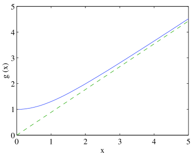
Figure 1: g$(x)$ and its asymptote.

where the temperatures of the two components are treated as equal. Since the integrals are spherically symmetric

$$\langle v_{r}(x)\rangle_{ij}={(\alpha/\pi)^{3}\over 8m}\rme^{-\alpha\left(\bar{p}_{i}^{2}+\bar{p}_{j}^{2}\right)}I_{Q}(\alpha/2,\alpha|{\bf\bar{p}}_{i}+{\bf\bar{p}}_{j}|)I_{Q}(\alpha/2,\alpha|{\bf\bar{p}}_{i}-{\bf\bar{p}}_{j}|),$$ (110)

where $I_{Q}(a,b)$ and $I_{q}(a,b)$ are discussed in B. In terms of the average thermal velocity (97) the final result may then be written as

$$\langle v_{r}(x)\rangle_{ij}=\bar{v}_{r}\;{\rm g}\left({|\bar{{\bf v}}_{i}-\bar{{\bf v}}_{j}|\over\bar{v}_{r}\sqrt{\pi/4}}\right),$$ (111)

where

$${\rm g}(x)={\rme^{-x^{2}}\over 2x}\left(x+(1+2x^{2}){\rme^{x^{2}}\sqrt{\pi}\over 2}{\rm erf}(x)\right).$$ (112)

Since ${\rm g}(0)=1$ this reproduces the standard result for a single component gas, and for the case where there is no mean relative motion of the two internal states. In the high relative velocity limit obtained by setting ${\bf\bar{v}}_{i}({\bf x})=-\bar{{\bf v}}_{j}({\bf x})={\bf\hat{x}}\bar{v}(x)$ with $\bar{v}_{r}\ll\bar{v}(x)$, the large $x$ limit ${\rm g}(x)\rightarrow\sqrt{\pi/4}x$ yields

$$\langle v_{r}(x)\rangle_{ij}\rightarrow 2\bar{v}(x).$$ (113)

Figure 1 shows the simple interpolation given by g. The effect of relative velocity on the relaxation may now be included by substituting (111) for the thermal result used in (104).

5.5.3 Variation with temperature

Since ${\rm g}(2)\simeq 2$, when the axial relative velocity is $\sqrt{\pi}\bar{v}_{r}\sim 1.7\bar{v}_{r}$ the damping rate will be doubled. For the JILA experiment the modification is somewhat less because the thermal velocity is of the order $\bar{v}_{r}\sim 20{\rm\;mms^{-1}}$, whereas the relative segregation velocity may be estimated to be at most $\sim 15{\rm\;mms^{-1}}$, corresponding to a $50\%$ increase in damping rate. This is expected to be important for the spin wave experiment since coherence damping has significant effects on the motion, and the coherence damping is also modelled using a simple relaxation time approximation. Moreover, if the experiments are attempted at higher temperatures this effect becomes more significant because the timescale for initiation of segregation scales like $\sim T^{-1/4}$ [5], and the cloud length scales like $\sim T^{1/2}$ so that the segregation velocity must behave like $\sim T^{3/4}$, whereas the thermal velocity scales like $\sim T^{1/2}$, so the ratio of the segregation velocity to the thermal velocity will be proportional to $\sim T^{1/4}$. Clearly this correction will become relatively less important for lower temperatures.

To find the effect of reducing the temperature on the coherence damping, we may compare the temperature dependence of the rates (100) and (90) with (94). In particular (100) and (90) are proportional to $\sqrt{k_{B}T}N({\bf x})$. The ratio of cubic to quadratic relaxation rates will vary as $NT^{-3/2}$, so that this process is expected to become more significant at lower temperatures. Since the peak density also varies as $T^{-3/2}$ the ratio will vary as $T^{-3}$. In particular, if the temperature is reduced by a factor of $3$ for the experimental parameters, the quadratic and cubic rates (90) and (94) will become similar. The cubic collision terms (5.4.2) will be important in this regime, and in the simplest approach, the relaxation time approximation (100) would need to be modified to account for the relaxation caused by (5.4.2), with $u_{ij}\simeq u_{12}$. One could also carry out moment equation calculations similar to those of Nikuni [9] for the cubic contribution to the damping in linearized spin equations, but this not pursued here.

6 Simulations

To simulate the experiment the equations (13,14,15) are reduced to an effective one dimensional description, and damping is included by adding the simple relaxation approximation term (105) to the resulting equations of motion.

6.1 Simplifications

The high anisotropy of the trap and low densities used allow the a reduction to a quasi-one dimensional model starting from a noninteracting initial condition. We may also take $\dot{N}({\bf x})=0$ as seen in the experiment, and verified by our simulations.

6.1.1 Initial motion

The state of the gas before the $\pi/2$ pulse, given by the Boltzmann distribution

$$n({\bf x},{\bf p})|_{t=0}={\cal N}\exp{\bigg{(}-{p^{2}\over 2mkT}-{V_{1}({\bf x})+2u_{11}N({\bf x})\over k_{B}T}\bigg{)}}$$ (114)

for the single internal state $|1\rangle$, is the stationary solution of the equation of motion

$$\dot{n}({\bf x},{\bf p})=\left\{-({\bf p}/m)\cdot\nabla_{\bf x}+\nabla(V_{1}({\bf x})+2u_{11}N({\bf x}))\cdot\nabla_{\bf p}\right\}n({\bf x},{\bf p}).$$ (115)

We may therefore neglect the density dependent effective potential $2u_{11}N({\bf x})$ if

$$\bigg{|}{2u_{11}\nabla N({\bf x})\over\nabla V_{1}({\bf x})}\bigg{|}={2u_{11}N({\bf x})\over k_{B}T+2u_{11}N({\bf x})}\leq{2u_{11}N({\bf x})\over k_{B}T}\ll 1.$$ (116)

For the densities used in our simulations $2u_{11}N(0)/kT\simeq 0.02$ allowing the use of the noninteracting initial condition. After the pulse the system consists of an equal superposition of two internal states in identical external configurations, so we simply use

$$n({\bf x},{\bf p})|_{t=0} = {\cal N}\exp{\bigg{(}-{p^{2}\over 2mkT}-{V_{1}({\bf x})\over k_{B}T}\bigg{)}},$$ (117)

$$m({\bf x},{\bf p})|_{t=0} = 0,$$ (118)

$$f({\bf x},{\bf p})|_{t=0} = {1\over 2}n({\bf x},{\bf p})|_{t=0}.$$ (119)

6.1.2 One dimensional equation

The high aspect ratio of the trap ($33:1$) means that there is a separation of timescales, leading to a physical transverse averaging of the atomic motion. This means that we may average the distributions over radial coordinates and momenta and find a one dimensional equation of motion. The only change is that the interaction strengths are divided by the transverse cross section of the sample given by $\pi R_{\perp}^{2}$ where the transverse radius $R_{\perp}$ is two standard deviations of the equilibrium density. A typical interaction dependent term has the form

$${\partial f({\bf x},{\bf p})\over\partial t}=u\;G({\bf x})f({\bf x},{\bf p}).$$ (120)

All of the terms can be seen to be either of this type, or to have no interaction parameter and therefore to be unaltered by the radial integration. Putting

$$f({\bf x},{\bf p}) = f(x,p)\left({m\omega_{r}^{2}\over 2\pi k_{B}T}\right)\exp{\left(-m\omega_{r}^{2}(y^{2}+z^{2})/2k_{B}T\right)}$$

$$\times\left({1\over 2\pi mk_{B}T}\right)\exp{\left(-(p_{y}^{2}+p_{z}^{2})/2mk_{B}T\right)},$$

$$G({\bf x}) = G(x)\left({m\omega_{r}^{2}\over 2\pi k_{B}T}\right)\exp{\left(-m\omega_{r}^{2}(x^{2}+y^{2})/2mk_{B}T\right)},$$ (121)

and integrating over radial momenta and coordinates leads to

$${\partial f(x,p)\over\partial t} = {u\over\pi(2\sqrt{\pi k_{B}T/m\omega_{r}^{2}})^{2}}\;G(x)f(x,p)$$ (122)

where the denominator is clearly the transverse cross-section of the sample, at a radius of two standard deviations. The effective scattering parameter has the dimensions of energy$\times$length required for a one dimensional interaction parameter.

6.2 The differential potential

The differential potential described by the parameter $\nu_{\rm diff}$ is defined by the experimenters [1] as

$$\nu_{\rm diff}={1\over 2\pi}\sqrt{{h\over m}\left\langle{d^{2}\nu_{12}\over dz^{2}}\right\rangle},$$ (123)

where the Gaussian weighted average of the frequency shift curvature is

$$\left\langle{d^{2}\nu_{12}\over dz^{2}}\right\rangle={\int_{-3\bar{x}/2}^{3\bar{x}/2}dz\;N(z){d^{2}\nu_{12}(z)\over dz^{2}}\over\int_{-3\bar{x}/2}^{3\bar{x}/2}dz\;N(z)},$$ (124)

and $\bar{x}$ is the half width at half maximum of the the axial density distribution

$$N(z)={1\over\sqrt{2\pi R^{2}}}\;\rme^{-z^{2}/2R^{2}},$$ (125)

given by $\bar{x}=R\sqrt{2\log{2}}$, where $R=\sqrt{k_{B}T/m\omega_{z}^{2}}$. It is apparent from Figure 2 of [1] that we can accurately represent the gradient of the differential potential in terms of a Gaussian with amplitude $A_{g}$ defined as

$$V_{\rm diff}(z)\equiv-A_{g}N(z).$$ (126)

We then obtain $A_{g}$ using (123),(124) and (126), to find

$$A_{g} = 4\pi R^{3}m\omega_{\rm diff}^{2}\left\{{{\rm erf}(3\bar{x}/2\sqrt{2}R)\over\sqrt{\pi}{\rm erf}(3\bar{x}/2R)+(3\bar{x}/R)\exp{\left(-(3\bar{x}/2)^{2}/R^{2}\right)}}\right\}$$ (127)

$$\simeq 4\pi R^{3}m\omega_{\rm diff}^{2}\times 0.44.$$

If we now expand (126) for small $z$ we find

$$-A_{g}N(z)\simeq{\rm constant}+{m\over 2}\left(\omega_{\rm diff}\sqrt{2}(2\pi)^{1/4}\sqrt{0.44}\right)^{2}z^{2},$$ (128)

so that the true frequency near the center of the trap is $\sim 1.49\nu_{\rm diff}$. Such a correction is expected since the Gaussian weighting process will reduce the resulting $\nu_{\rm diff}$ by adding in negative frequencies, if the range of integration is taken beyond the turning point of the Gaussian $N({\bf x})$.

6.3 Results

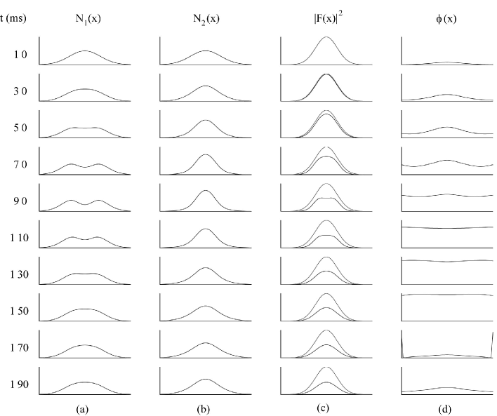
Figure 2: Time is in ms down the left column. $N(0)=1.16\times 10^{13}{\rm cm}^{-3}$, $T=850$nK, $\nu_{\rm diff}=0.1$. (a) and (b) are the densities of the two internal states in arbitrary units. (c) Shows the coherence density, with initial condition for comparison, and d) shows the relative phase between the two internal states $\phi(x)={\rm angle}(F(x))$; the plot range is $[0,2\pi)$.

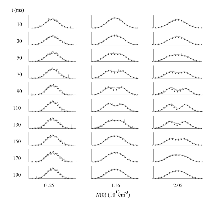
Figure 3: Measured $N_{1}(z)$, with simulations (dotted line) for $\nu_{\rm diff}=0.1$ and peak densities listed at the foot of each column. Time is in ms down the left column.

Figure 2 shows the result of simulating equations (13,14,15) with $\nu_{\rm diff}=0.16\;{\rm Hz},N(0)=1.8\times 10^{13}{\rm cm}^{-3}$, with the relaxation time approximation (105) modelling the damping. The effect is very similar to that seen in the experiment [1]. In (a) and (b) the axial density profile of the $|1\rangle$ and $|2\rangle$ states show a clear axial segregation of the two internal states. (c) Shows the decay of the coherence which causes the transience of the phenomena on the timescale of the experiment. The initial condition is shown for comparison. Column (d) is the phase of $F({\bf x})$, from which it is clear that the relative motion tends to smooth out the relative phase gradient that is caused by the differential potential $V_{\rm diff}({\bf x})$.

Figure 3 shows the results of simulations for the experimental parameters, with the measured data [10]. The timescale for decay of coherence is well described by the simple relaxation time approximation, with an extra factor of 2. The initiation times, relaxation times and amplitude of the segregation agree qualitatively with the experiment.

Figure 4 shows the variation with $\nu_{\rm diff}$, and the numerical results. We see here that what is described as ”higher order effects” are not well modelled by the simulation for $\nu_{\rm diff}=0.20\;{\rm Hz}$. The initiation time and transience are still in good agreement but the extra peak in the center of $N_{1}(x)$ does not emerge.

6.4 ‘Classical’ Motion

It is useful to consider the classical motion that would arise if the system could be prepared with identical initial state distributions as constructed by the first $\pi/2$ pulse of the experiment, while also setting the coherence to zero. If coherence is neglected the initial condition (114) is merely a density perturbation from the new Boltzmann equilibrium

$$n({\bf x},{\bf p}) = {\cal N}\exp{\left(-{p^{2}\over 2mk_{B}T}-{V_{\rm eff}({\bf x})\over k_{B}T}\right)}\cosh{\left({V_{\rm diff}({\bf x})\over k_{B}T}\right)},$$

$$m({\bf x},{\bf p}) = {\cal M}\exp{\left(-{p^{2}\over 2mk_{B}T}-{V_{\rm eff}({\bf x})\over k_{B}T}\right)}\sinh{\left({V_{\rm diff}({\bf x})\over k_{B}T}\right)}.$$ (129)

The corresponding single species distributions are

$$n_{1}({\bf x},{\bf p}) = {\cal N}_{1}\exp{\left(-{p^{2}\over 2mk_{B}T}-{V_{1}({\bf x})+2u_{11}N_{1}({\bf x})+u_{12}N_{2}({\bf x})\over k_{B}T}\right)},$$

$$n_{2}({\bf x},{\bf p}) = {\cal N}_{2}\exp{\left(-{p^{2}\over 2mk_{B}T}-{V_{2}({\bf x})+2u_{22}N_{2}({\bf x})+u_{12}N_{1}({\bf x})\over k_{B}T}\right)}$$

for appropriate normalizations ${\cal N}_{1}$ and ${\cal N}_{2}$. We have seen in section 6.1.1 that the interactions have a negligible effect on the initial condition, and similar reasoning shows the equilibrium segregation after the pulse is negligible for the densities used in the experiment [1]. It follows that the classical motion towards the new equilibrium would be small, as long as the fluctuations caused by the perturbation are also small.

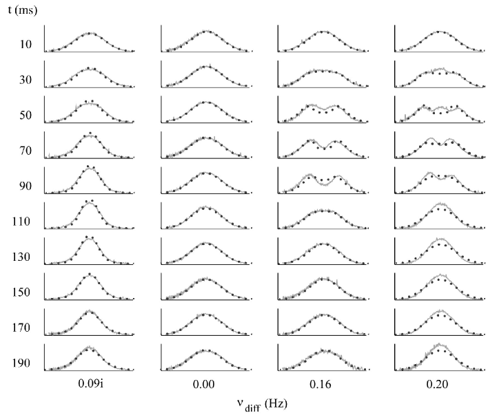
Figure 4: Measured $N_{1}(z)$, with simulations (dotted line) for peak density $N(0)=1.8\times 10^{13}\;{\rm cm}^{-3}$ and $\nu_{\rm diff}$ listed at the foot of each column. Time is in ms down the left column.

7 Spin waves and atomic motion

In the experimental report it is asserted that the motion observed must be due to actual physical motion of the atoms since energy conservation would seem to prohibit spontaneous interconversion of the internal states [1]. In this situation ‘motion’ refers to the redistribution of the atomic density in the trap. The issue is whether or not it is possible to distinguish between two interpretations: The apparent motion is the result of either

• Transport of the atoms in the relative phase gradient arising from the Zeeman and mean field effects, or

• The coherent interconversion of the internal states as a result of the interactions.

In defence of the first picture, it has been suggested in [1] that the rate of segregation can be accounted for if the small differential potential is somehow amplified in a coherent collision processes which channels the thermal energy of atoms in a particular direction. In the second picture, the collisions between the two different internal states are interpreted as causing a rotation in pseudo-spin space of the spinor wave function for the two state superposition of the field operators.

It is important to note here that if the transport terms are neglected in the equations of motion, segregation does not occur. The equations of motion for the densities are found by integrating the equations of motion (13), (14), (15) over momentum which leads to

$$\dot{N}({\bf x})+\nabla\cdot(N({\bf x}){\bf v}_{N}({\bf x})) = 0$$ (131)

$$\dot{M}({\bf x})+\nabla\cdot(M({\bf x}){\bf v}_{M}({\bf x})) = 0$$ (132)

$$\dot{F}({\bf x})+\nabla\cdot(F({\bf x}){\bf v}_{F}({\bf x})) = -i\omega_{R}({\bf x})F({\bf x}),$$ (133)

where the velocities are, for example

$${\bf v}_{N}={1\over mN({\bf x})}\int d^{3}{\bf p}\;{\bf p}\;n({\bf x},{\bf p}),$$ (134)

and the Ramsey frequency is $\omega_{R}({\bf x})=\Delta\omega_{c}({\bf x})+\Delta\omega_{z}({\bf x})$.

If the transport terms are neglected the velocities vanish, and no change in the densities can occur—the only effect is to make a redistribution in momentum space. Inclusion of the transport terms then translates this redistribution in momentum space into a redistribution in position. In this sense, we agree with the view of [1] that the segregation is caused by actual motion of the atoms. The effect is however quite large, since it involves more forces than simply the classical forces induced by the gradient of the differential potential, namely the forces caused by the production of a spatially dependent phase of $f({\bf x},{\bf p})$, as seen in the second line of (15).

8 Comparison with other work

While preparing this work several other papers on the JILA experiment [1] have appeared [3, 4, 5]. The works [5, 4] use essentially the same formalism as our own, with slightly different degrees of approximation. In [5] the simulations agree with experiment to the same quantitative degree as our own, although they obtain better results for the variation of $\nu_{\rm diff}$, in particular we do not see higher order effects for the highest value $\nu_{\rm diff}=0.2\;{\rm Hz}$ as reported in the experiment and found by Williams et al [5]. In [4] the simulated initiation times appear more rapid than seen in the experiment. Our results show better agreement for this feature, which may be because we have inverted the curvature averaging process used to characterize the differential potential. In [5, 4] the timescale of initiation for the segregation is found analytically, and in [5] it is noted that this also gives the position of the nodes of $M({\bf x})$. In [3] a so called Landau-Lifshitz equation of motion was obtained, and solved numerically, finding qualitatively similar behavior, although the timescale of evolution is significantly longer than that observed in the experiment.

More recent work at JILA [8] has focused on providing data for a collective mode analysis which has been carried out by Nikuni et al [9] using a truncated moment equation approach. In this experiment the differential potential is controllable in real time, so that a small amplitude fluctuation may be excited, and the potential gradient then set to zero for the remainder of the motion. The same relaxation time approximation is used to that derived here, and the simulations of [9] show excellent agreement with the data of [8]. Some discrepancy is found for the quadrupole mode in the regime where Landau damping is the dominant form of dissipation, and the authors note that the details of the trap are likely to be important in describing this process accurately.

9 Conclusions

We have simulated the JILA experiment using the Wigner function approach and found reasonable agreement with the data of [1]. We have discussed the Ramsey frequency and the local transition frequency for this system, and emphasized the difference of the two, finding that the Ramsey technique is insensitive to the decay of coherence. A relaxation time approximation for the experiment has been derived, including the effect of relative velocity which is expected to be important for higher temperature experiments. A Quantum Boltzmann collision term for two species with arbitrary S-wave interaction strengths was found, and we evaluated the effects of scattering on the coherence for non-condensed $\phantom{|}{}^{87}{\rm Rb}$  using a Boltzmann equilibrium form for the momentum distributions. It is apparent that the cubic terms in the collision integral depend on the phase space density and will be important for more degenerate regimes.

Appendix A Continuum limit

The derivation of (5.2) from the terms (82) and (83) is simplified by the identities of the form

$$\sum_{ijIJ,{\bf e}}\delta(\Delta\omega({\bf e}))\langle U_{IJ}^{\dagger}({\bf e})[\psi^{\dagger}_{l{\bf k}}\psi_{m{\bf k}},U_{ij}({\bf e})]\rangle^{*}=\sum_{ijIJ,{\bf e}}\delta(\Delta\omega({\bf e}))\langle[U_{ij}({\bf e}),\psi^{\dagger}_{m{\bf k}}\psi_{l{\bf k}}]U_{IJ}^{\dagger}({\bf e})\rangle$$

so that (82) and (83) are complex conjugates with $l\leftrightarrow m$. The Quantum Boltzmann equation (5.2) is then obtained by using

$$f_{lm}({\bf k}) = \left({\pi\over\Delta}\right)^{3}\sum_{{\bf N}}{\rm Tr}\{v_{{\bf N}}\psi^{\dagger}_{l{\bf k}}\psi_{m{\bf k}}\}$$ (136)

$$= \left({\pi\over\Delta}\right)^{3}\langle\psi^{\dagger}_{l{\bf k}}\psi_{m{\bf k}}\rangle,$$

so that the commutators may be evaluated and we may carry out the procedures in [7] for passing to the continuum limit. This involves factorizing the operator averages and using the local equilibrium forms

$$\langle\psi^{\dagger}_{l{\bf K}_{1}}({\bf x})\psi_{m{\bf K}_{2}}({\bf x^{\prime}})\rangle = {\rm g}({\bf x}-{\bf x^{\prime}})\;f_{lm}\left({{\bf x}+{\bf x^{\prime}}\over 2},{\bf K}_{1}\right)\delta_{{\bf K}_{1},{\bf K}_{2}}$$ (137)

$$\langle\psi_{l{\bf K}_{1}}({\bf x})\psi^{\dagger}_{m{\bf K}_{2}}({\bf x^{\prime}})\rangle = {\rm g}({\bf x}-{\bf x^{\prime}})\left(f_{ml}\left({{\bf x}+{\bf x^{\prime}}\over 2},{\bf K}_{1}\right)+\delta_{lm}\right)\delta_{{\bf K}_{1},{\bf K}_{2}},$$ (138)

and the continuum limit of the summation

$$\sum_{{\bf K}_{2},{\bf K}_{3},{\bf K}_{4}} \left({\pi\over\Delta}\right)^{3}M_{\Delta}({\bf K}+{\bf K}_{2}-{\bf K}_{3}-{\bf K}_{4})$$ (139)

$$\rightarrow{1\over(2\pi)^{6}}\int\;d^{3}{\bf K}_{2}\int\;d^{3}{\bf K}_{3}\int\;d^{3}{\bf K}_{4}$$

$$\times\delta({\bf K}+{\bf K}_{2}-{\bf K}_{3}-{\bf K}_{4}),$$

where

$${\rm g}({\bf x})={1\over\pi^{3}}\left[{\sin{\Delta x}\over x}\right]\left[{\sin{\Delta y}\over y}\right]\left[{\sin{\Delta z}\over z}\right],$$ (140)

and $M_{\Delta}({\bf Q})$ is the approximate delta function arising from the factorization of operator averages

$$M_{\Delta}({\bf Q}) = \int\;d^{3}{\bf y}\int\;d^{3}{\bf y^{\prime}}{\rm g}({\bf y}){\rm g}({\bf y^{\prime}})[{\rm g}({\bf y}-{\bf y^{\prime}})]^{3}\rme^{i{\bf Q}\cdot({\bf y}-{\bf y^{\prime}})}$$ (141)

$$= \prod_{i=1}^{3}\left({\Delta\over\pi}\right)^{3}\left\{{2\over 3}\delta_{Q_{i},0}+{1\over 3}\delta_{Q_{i},\Delta}+{1\over 3}\delta_{Q_{i},-\Delta}\right\}.$$

(This corrects an error in Eqs. (128) and (129) of [7], which led to an extra factor of $(2\pi)^{3}$ in the final Uehling-Uhlenbeck collision term (132)).

Appendix B Integrals

Some useful integrals for this paper are

$$I_{Q}(a,b) = \int_{0}^{2\pi}d\phi\int_{0}^{\pi}\;d\theta\;\sin\theta\int_{0}^{\infty}dQ\;Q^{2}\rme^{-aQ^{2}+bQ\cos\theta}$$ (142)

$$= {2\pi\sqrt{\pi}\over ab}\left({b\over 2\sqrt{a}}\right)\exp{(b^{2}/4a)}$$ (143)

and

$$I_{q}(a,b) = \int_{0}^{2\pi}d\phi\int_{0}^{\pi}\;d\theta\;\sin\theta\int_{0}^{\infty}dq\;q^{3}\rme^{-aq^{2}+bq\cos\theta}$$ (144)

$$= {2\pi\rme^{b^{2}/4a}\over a^{2}}\;{\rm g}\left(b/2\sqrt{a}\right),$$ (145)

where

$${\rm g}(x)={\rme^{-x^{2}}\over 2x}\left(x+(1+2x^{2}){\rme^{x^{2}}\sqrt{\pi}\over 2}{\rm erf}(x)\right).$$ (146)

Defining

$$B({\bf p})\equiv(2\pi\hbar)^{3}\left({\alpha\over\pi}\right)^{3/2}\exp{(-\alpha{\bf p}^{2})}$$ (147)

the integral

$$I_{34} \equiv \int\;d^{3}{\bf P}_{1}\int\;{d^{3}{\bf P}_{2}\over(2\pi\hbar)^{3}}\int\;{d^{3}{\bf P}_{3}\over(2\pi\hbar)^{3}}\int\;{d^{3}{\bf P}_{4}\over(2\pi\hbar)^{3}}B({\bf P}_{3})B({\bf P}_{4})$$ (148)

$$\;\;\;\;\;\;\;\;\;\;\;\;\;\;\times\delta({\bf P}_{1}+{\bf P}_{2}-{\bf P}_{3}-{\bf P}_{4})\delta(\epsilon_{1}+\epsilon_{2}-\epsilon_{3}-\epsilon_{4})$$

is found by using the transformation ${\bf Q}={\bf P}_{1}+{\bf P}_{2}$, ${\bf q}={\bf P}_{1}-{\bf P}_{2}$ to obtain

$$I_{34} = {m\over 2^{4}(2\pi\hbar)^{3}}\left({\alpha\over\pi}\right)^{3}\int\;d^{3}{\bf Q}\int\;d^{3}{\bf K}\int\;d^{3}{\bf q}\int\;d^{3}{\bf k}\;\exp{(-\alpha({\bf Q}^{2}+{\bf q}^{2})/2)}$$ (149)

$$\;\;\;\;\;\;\;\;\;\;\;\;\;\;\times\delta({\bf q}^{2}-{\bf k}^{2})\delta({\bf Q}-{\bf K})$$

$$= {2\pi m\over 2^{4}(2\pi\hbar)^{3}}\left({\alpha\over\pi}\right)^{3}I_{Q}(\alpha/2,0)I_{q}(\alpha/2,0)=\sqrt{2\pi\over\alpha}{2m\over(2\pi\hbar)^{3}}.$$

The integral $I_{234}$ is found in a similar fashion as

$${\rm I}_{234} \equiv \int\;{d^{3}{\bf P}_{1}\over(2\pi\hbar)^{3}}\int\;{d^{3}{\bf P}_{2}\over(2\pi\hbar)^{3}}\int\;{d^{3}{\bf P}_{3}\over(2\pi\hbar)^{3}}\int\;d^{3}{\bf P}_{4}\;B({\bf P}_{2})B({\bf P}_{3})B({\bf P}_{4})$$ (150)

$$\;\;\;\;\;\;\;\;\;\;\;\;\;\;\times\delta({\bf P}_{1}+{\bf P}_{2}-{\bf P}_{3}-{\bf P}_{4})\delta(\epsilon_{1}+\epsilon_{2}-\epsilon_{3}-\epsilon_{4})$$

$$= {\sqrt{3}\over 4\pi k_{B}T}.$$

References

References

• [1] H.Β J. Lewandowski, D.Β M. Harber, D.Β L. Whitaker and E.Β A. Cornell, Phys. Rev. Lett 88, 070403 (2002).
• [2] C. W. Gardiner, A. S. Bradley, J. Phys. B 34, 4673-4687, (2001)
• [3] M. O. Oktel, L. S. Levitov, Phys. Rev. Lett. 88, 230403 (2002).
• [4] J. N. Fuchs, D. M. Gangardt, F. Laloe, Phys. Rev. Lett. 88, 230404 (2002).
• [5] J. E. Williams, T. Nikuni, C. W. Clark, Phys. Rev. Lett. 88, 230405 (2002).
• [6] L.Β E. Reichl, A Modern Course in Statistical Physics (University of Texas Press, USA, 1980).
• [7] C.Β W. Gardiner, P. Zoller, Phys. Rev. A 55, 2902 (1997).
• [8] J. M. McGuirk, H. J. Lewandowski, D. M. Harber, T. Nikuni, J. E. Williams and E. A. Cornell, Phys. Rev. Lett. 89, 090402 (2002).
• [9] T. Nikuni, J. E. Williams and E. A. Cornell, cond-mat/0205450.
• [10] We use the raw data quoted in cond-mat/0112487.
• [11] D. M. Harber, H. J. Lewandowski, J. M. McGuirk and E. A. Cornell, cond-mat/0208294.