Scaling Properties of 1D Anderson Model with Correlated Diagonal Disorder

Abstract

Statistical and scaling properties of the Lyapunov exponent for a tight-binding model with the diagonal disorder described by a dichotomic process are considered near the band edge. The effect of correlations on scaling properties is discussed. It is shown that correlations lead to an additional parameter governing the validity of single parameter scaling.

I Introduction

It has been known for almost forty years that in standard one-dimensional disordered models all states are localized for any strength of disorder, and that there is no localization transition in such systems.gang ; LGP Formally this is expressed by the statement that the Lyapunov exponent (LE), $\gamma$, defined as

$$\gamma=-\lim_{L\rightarrow\infty}\frac{1}{2L}\ln{T},$$ (1)

where $T$ is the transmission coefficient through the system of length $L$, is always positive.LGP While it may seem that there is nothing more to be said about one-dimensional models, their localization properties have recently attracted a great deal of attention. This renewed interest has been concentrated in two areas. The first area includes studies of unusual models that demonstrate the presence of extended states. It was noted first in Ref. dimer, that introducing correlations in the statistical properties of random site energies in the Anderson model, one can create extended states in the one-dimensional Anderson model at certain values of energy. Later on, the authors of Ref. Moura, showed that regions of extended states exist in 1D systems with long range correlations of the random potential. The authors of Ref. Izrailev, demonstrated that vanishing LE can be obtained in an arbitrarily chosen spectral region by selecting a special form of the correlation function of the random potential. It should be noted, however, that this result was obtained in Ref. Izrailev, only in the second order of the weak disorder expansion. Taking into account the next terms of the expansion makes LE positive again.fourth order pt

The second area of research interest in the field of one-dimensional localization is focused upon scaling and statistical properties of finite size systems. The single parameter scaling put forward in Ref. gang, is a cornerstone of the current approach to the Anderson localization, but its interpretation in the presence of non-self-averaging fluctuations of conductivity was the subject of long debate. Eventually it was understood that the SPS hypothesis in Anderson localization means that the entire distribution function of conductivity (or transmission), and not individual moments, must be parameterized by a single parameter.Anderson ; Shapiro This distribution in one-dimensional systems has been intensively studiedKramerReview , and it was established that the bulk of the distribution for sufficiently long systems has a log-normal form. It was also understood starting with Ref. Anderson, that under certain circumstances the two parameters of the distribution, the average value of the finite size LE, $\tilde{\gamma}=-\ln{T}/(2L)$, which coincides with its limiting value, $\gamma=\langle\tilde{\gamma}\rangle$, and the variance, $\sigma^{2}=var(\tilde{\gamma}),$ are related to each other in a universal way

$$\tau=\frac{\sigma^{2}L}{\gamma}=1.$$ (2)

This relation reduces two parameters of the distribution to only one, and provides, therefore, a justification and interpretation for SPS. Conditions, under which Eq. (2) holds, however, have been established only recently, when the authors of Ref. PRLclassics, showed that the validity of SPS is controlled by a new macroscopic length, $l_{s}$, defined in terms of the integral density of states, $N(E)$:

$$l_{s}^{-1}=\sin{(\pi N(E))}.$$ (3)

where $E$ is energy. It was shown that SPS holds when $\kappa=(\gamma l_{s})^{-1}>1$, and fails in the opposite case. Recently, the authors of the present paper showed that parameter $\kappa$ plays a more important role than just establishing the criterion for SPS. It was found that in the non-SPS region the function $\tau$ defined in Eq. (2), and the similar dimensionless combination of the third moment with the length $L$ and the Lyapunov exponent $\gamma$ are functions of this single parameter.nonSPSlast In the recent paper Ref. Titov, , higher moments of the distribution of the Lyapunov exponent were calculated analytically for a quantum particle in a potential described by the Gaussian delta-correlated random function. It was found that all moments of the distribution for this model can be expressed as functions of the localization length and the parameter $E/D^{2/3}$ , where $D$ characterizes the strength of the potential. For the Gaussian white noise potential the parameter $\kappa$ is also a function of $E/D^{2/3},$PRLclassics thus in the particular case of the Gaussian white noise potential these two parameters are equivalent.

In the present paper, we combine the two discussed areas and focus upon correlation induced changes in the probability distribution function of the Lyapunov exponent. In order to study this problem, we consider a tight-binding model with the random potential described by a zero-mean dichotomic process. This process is characterized by an exponential correlation function with a correlation radius, which is a free parameter of the model. There is no localization-delocalization transition in this model, and we are interested in effects of the correlation radius on scaling and statistical properties of conductance in the regime of strongly localized states. This model allows for an approximate analytical treatment in the spectral region, where the correlation radius becomes a dominant length. Combining analytical and numerical calculations we show that the presence of this additional length significantly changes the transition between SPS and non-SPS regions, and that in the non-SPS region it results in a new scaling behavior.

II Quasiclassical approximation for Lyapunov exponent

We consider the tight binding model, described by the equation of motion

$$\psi_{n+1}+\psi_{n-1}+(V\zeta_{n}-E)\psi_{n}=0,$$ (4)

where $V$ describes the strength of the random potential. The potential randomly takes one of two values $\pm V$ depending upon whether the dichotomic random variable $\zeta_{n}$ is equal to $1$ or $-1$. The assumed value remains constant within regions of random lengths (segments), which are distributed according to the discrete analog of the Poisson distribution. The average length of such regions is

$$l_{c}=\coth\left(\frac{1}{2r_{c}}\right),$$ (5)

where $r_{c}$ is the correlation radius defined by

$$\left\langle\zeta_{n}\zeta_{m}\right\rangle=e^{-|n-m|/r_{c}}.$$ (6)

The finite size LE is defined through the norm of the transfer matrix:

$$\tilde{\gamma}(E)=\frac{1}{L}\log\left\|T_{N}\ldots T_{1}\right\|,$$ (7)

where $T_{n}$ are transfer matrices which, in our case, are equal to either $T_{+}$, or $T_{-}$ depending upon the value of $\zeta_{n}$, where $T_{\pm}$ are

$$T_{\pm}=\left(\begin{array}[]{cc}E\pm V&-1\\ 1&0\end{array}\right).$$ (8)

To consider the spectrum of this system let us note that an addition of a constant potential $\pm U$ shifts a conduction band, $-2\leq E\leq 2$, of the homogeneous tight-binding system with no on-site potential by the value of the potential: $-2\mp U\leq E\leq 2\mp U$. Correspondingly, the spectrum of the random system under consideration can be divided into three regions with the qualitatively different spectral and transport properties. One region, $0<|E|<2-V$, corresponds to the common part of the conduction bands of homogeneous systems with the site potentials equal to either $+V$ or $-V$.  In the second spectral region, consisting of energies $2-V<E<2+V$ and $-2-V<E<-2+V$, extended states exist in a homogeneous system with the site potentials equal to $-V$ or $+V$, respectively. Finally the third region, $2+V<|E|$ corresponds to the energies, where extended states would not arise in homogeneous systems with either of the two possible values of the potential. Obviously, no states can arise in this region also in the system with the random distribution of the potential.

While all states in this model are localized, different spectral regions still have different transport properties. Transport in the first region is characterized by multiple scattering of propagating modes, and the localization in this region results from the interference of the scattered waves. Transport in the second region can be described as tunneling through states, arising within the segments of the system, where the potential produces potential wells between barriers formed by segments with the opposite value of the potential. If the average length of the “barrier” regions is larger than the penetration length under the barrier, the transport is mostly determined by the under-barrier tunneling, and the interference effects related to phase changes of the wave functions inside potential wells become less important. We are mostly interested in this region, where correlations are expected to result in the most non-trivial effects. One could expect that the transport in this region can be described within the quasi-classical approximation, and we will show below that this is indeed the case.

In the context of our problem, this approximation means neglecting commutators between transfer matrices at different sites. Introducing LE in a homogeneous system with the potential $U$ according to

$$\gamma_{0}(E;U)=\mathrm{Re}\left[\lambda_{0}(E;U)\right],$$ (9)

where

$$\lambda_{0}=\cosh^{-1}\left(\frac{E-U}{2}\right),$$ (10)

we can write a quasiclassical expression for LE for Eq. (4) in the following form

$$\tilde{\gamma}(E)\approx\frac{1}{L}\sum_{n=1}^{N}\gamma_{0}(E;V\zeta_{n}).$$ (11)

Using the fact that the $\zeta_{n}=\pm 1$, Eq. (11) can be rewritten in the form

$$\tilde{\gamma}=\gamma_{a}+\frac{\delta}{L}\sum_{n=1}^{N}\zeta_{n},$$ (12)

where

$$\gamma_{a} = \frac{1}{2}\left[\gamma_{0}(E;V)+\gamma_{0}(E;-V)\right],$$

$$\delta = \frac{1}{2}\left[\gamma_{0}(E;V)-\gamma_{0}(E;-V)\right].$$ (13)

The averaged finite-length LE, $\gamma=\left\langle\tilde{\gamma}\right\rangle$, is determined by $\gamma_{a}$, while its variance $\sigma^{2}$ depends upon $\delta$:

$$\sigma^{2}=\left\langle\gamma^{2}\right\rangle-\left\langle\gamma\right\rangle^{2}=\frac{\delta^{2}}{L}l_{c}.$$

In the first spectral region this approximation yields vanishing LE, which is quite understandable, because interference effects responsible for the localization in this region are completely neglected.

Eq. (11) can be formally obtained in the following way. The relation between LE and the eigenvalues of the transfer matrix allows us to write

$$2\cosh(\tilde{\gamma}L)=\mathrm{Tr}\,\left(T_{N,1}\right).$$ (14)

where the transfer matrix $T_{N,1}$ consists of sequences of $T_{\pm}$

$$T_{N,1}=T_{N}\ldots T_{1}=\ldots T_{+}^{n_{3}}T_{-}^{n_{2}}T_{+}^{n_{1}},$$ (15)

Powers $n_{k}$ of transfer matrices $T_{\pm}$ represent the lengths of the regions where the potential remains constant. The matrices $T_{\pm}$ can be diagonalized $T_{\pm}^{n}=R_{\pm}S_{\pm}^{n}R_{\pm}^{-1}$, where

$$S_{\pm}^{n}=\left(\begin{array}[]{cc}e^{\lambda_{0}(\pm V)n}&0\\ 0&e^{-\lambda_{0}(\pm V)n}\end{array}\right)$$ (16)

Thus, introducing $\alpha_{12}=R_{+}^{-1}R_{-}$ and $\alpha_{21}=R_{-}^{-1}R_{+}$, and noting that for long enough samples the effect of matrices $R_{\pm}$ appearing at the end of the structure on LE is negligible, we obtain that LE can be found from Eq. (14) with the transfer matrix replaced by

$$\tilde{T}_{N,1}=\ldots\alpha_{21}S_{+}^{n_{2}}\alpha_{12}S_{-}^{n_{1}}.$$ (17)

The last step in the procedure is to commute, for example, $S_{+}$ and $\alpha_{12}$, with the purpose of collecting all $S_{\pm}$ together. If one begins this rearrangement from the right side of Eq. (17), each of such permutations produces two terms. One of them consists of the product of the partially ordered and the remaining non-ordered parts, while the second one contains commutators of $S_{+}$ and $\alpha_{12}$. Repeating the procedure leads to the recurrent equation for the part of the transfer matrix containing only products of commuting diagonal matrices $S_{\pm}$

$$T_{N,1}=\mathcal{O}_{N,1}+\sum_{k\in\mathrm{even}}T_{N,p_{k+1}}\Gamma_{n_{k}}\mathcal{O}_{p_{k-1},1},$$ (18)

where we have used the fact that $\alpha_{12}\alpha_{21}=1$, and introduced the commutator $\Gamma_{n}=\left[S_{+}^{n},\alpha_{12}\right]$. Notation $\mathcal{O}_{p_{k-1},1}$ stays for the product of all $S_{\pm}$ between sites $1$, and $p_{k-1}$: $\mathcal{O}_{N,1}=\ldots S_{+}^{n_{2}}S_{-}^{n_{1}}$, where $p_{k}=\sum_{l=1}^{k}n_{l}$.  Retaining the first term only and using Eq. (14) we arrive at Eq. (11).

Eq. (18) can be used to obtain a representation for the transfer matrix in terms of the polynomial in powers of the parameter $\delta$, which enters the expression for commutators $\Gamma_{n}$, and can be considered as a small parameter in the case of weak disorder. However, the resulting expression for the transfer matrix cannot be interpreted as a weak disorder expansion for LE. The reason for this is the fact that the power of $\delta$ is determined by the number of segments with different values of the potential, and the whole polynomial is actually an expansion in terms of the number of “jumps” between $V$ and $-V$. For instance, the term with $\delta^{2}$ results from configurations with only one such jump, and there are only $N$ such configurations. In the limit $N\rightarrow\infty$ they give zero correction to the LE (in addition to the exponentially small probability of such configurations). Thus, we can see that for long enough samples only terms of the order of $\mathcal{N}\sim N/2$ make a significant contribution to the LE because the number of such terms is proportional to the binomial coefficient $C_{N}^{\mathcal{N}}$ and, therefore they give a linear in $N$ contribution to the $\log\left\|T\right\|$. The actual number of configurations contributing to LE depends upon the average length of the segments with constant potential; and the number of jumps, corresponding to the optimal configurations can be estimated as $N/l_{c}$. It is clear, therefore, that corrections to the first term of Eq. (18) decrease with increasing $l_{c}$. We thus expect that the approximation should work when $l_{loc}/l_{c}\ll 1$. It actually becomes exact in the limit of infinite $r_{c}$ and $V.$Pastur_Figotin ; LargeCoupling This can be understood from the following arguments. Deviations from Eq. (12) are caused by the interference of the scattered waves. But in the second spectral region such scattered waves have to tunnel through the barriers, where the magnitude of the scattered waves decreases and the interference is destroyed. Obviously, the effectiveness of the destruction depends on the width of the potential barriers, and the rate of decay of the wave functions in them. These characteristics are determined by $l_{c}$ and the magnitude of the potential respectively.

In the spectral region, $2-V<|E|<2+V$ only $\gamma_{0}(E;V)$ in Eq. (II) is different from zero, and we have for $\sigma^{2}$

$$\sigma^{2}L=\gamma^{2}l_{c}.$$ (19)

This expression is obviously different from SPS Eq. (2), and is valid when $\gamma l_{c}\gg 1$. In this case, scaling described by the function $\tau(\kappa)$ is no longer valid, but Eq. (19) suggests that a new type of scaling appears. It can be conveniently described with the help of a new scaling function, $S$,

$$S=\frac{\sigma^{2}L}{\gamma^{2}l_{c}}\sim 1.$$ (20)

The transition between the two scaling regimes is controlled by the parameter $\gamma l_{c}$. If the correlation radius is so small that this parameter remains much less than unity for the entire second spectral region, the regular scaling behavior expressed by $\tau(\kappa)$ persists. The behavior expressed by Eq. (20) occurs when $\gamma l_{c}$ is greater than unity for the entire region $2-V<|E|<2+V$. More detailed analysis of the transition between the two types of behavior requires a numerical approach, which we discuss in the next section of the paper.

Figure 1: Dependence of the mean of the Lyapunov exponent on energy: numerical result (dotted line) and theory (solid line), for potential $V=0.4$ and correlation radius $r_{c}=10$.

In the third spectral region, $|E|>2+V$, $S$ decreases with energy. This behavior can be approximately described as

$$S\approx\frac{\left(\sqrt{2}\sqrt{|\epsilon|-1}-1\right)^{2}}{\left(\sqrt{2}\sqrt{|\epsilon|-1}+1\right)^{2}}$$ (21)

for $0<|\epsilon|-1\ll 1$, where $\epsilon=(2-|E|)/U$ and

$$S\approx\left(\frac{1}{\epsilon}\right)^{2}\frac{1}{(\log|U|+\log|\epsilon|)^{2}}$$ (22)

for $|\epsilon|\gg 1$.

III Scaling properties of LE: numerical simulations

For the numerical analysis, we calculate the LE iteratively using Eq. (7) and the usual technique of renormalization of the resultant vector after every 10 iterations.Kramer The length $l_{s}$ was calculated according to Eq. (3), where the integrated density of states was obtained using the phase formalism LGP with consequent averaging over all realizations. To investigate scaling properties we kept the length of chains much larger than the correlation length, $l_{c},$ and the localization length, $l_{loc},$ for all magnitudes of the random potential $U$ and values of the energy $E$ in the vicinity of the second spectral region. Statistics were collected from $40000$ realizations. Figs. 1a and b present results of numerical computations of the Lyapunov exponent. The numerical value of the correlation radius in these figures is such that $l_{c}>l_{loc}$ for the entire $2-V<|E|<2+V$ spectral region. A comparison of numerical results and the approximation (11) is provided for both average LE and its variance. For energies inside the first region this approximation gives zero, as discussed above. In the second region, one can see that Eq. (11) provides a reasonably good approximation for $\gamma$, and even better agreement for $\sigma^{2}$. In the third spectral region the agreement between Eq. (11) and the numerical calculations becomes perfect.

We also studied numerically the scaling properties of our model. Let us recall that for systems without correlations SPS is controlled by the ratio $\kappa=l_{loc}/l_{s}$ of two macroscopic lengths existing in the system. In the presence of the correlated disorder the situation is more complicated because a new length related to the correlation radius $r_{c}$ should be taken into account. In our model this length is $l_{c}-$ the average length of regions with constant potential. If $l_{c}$ is the smallest length in the system, $l_{c}<(l_{loc},l_{s}),$ the presence of correlations does not affect the scaling properties. Computer simulations show that the scaling parameter $\tau$ behaves in this case qualitatively similar to a system with uniformly distributed non-correlated disorder. In Fig. 2 the dependence of $\tau$ on $\kappa$ is shown for both a tight-binding model with uniformly distributed ($-U\leq V_{n}\leq U$) on-site potential (with $U$ ranging from $0.09$ to $0.145$) and the model under consideration. For the latter, potentials ($V=0.001-0.004$) and correlation radii ($r_{c}=2$ and $3$) where chosen such as to have $l_{c}$ the smallest length up to the genuine spectral boundary.

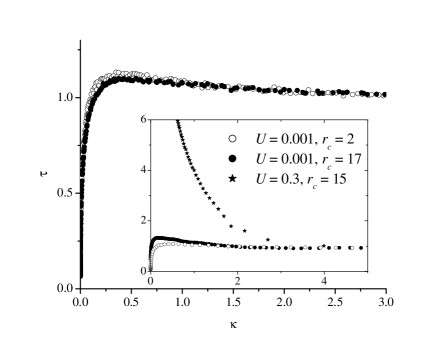
Figure 2: $\tau(\kappa)$ for different distributions of the potential: the uniform distribution (empty circles) and the dichotomic process (filled circles) when $r_{c}$ is the smallest length of the system.

However, when $l_{c}>l_{loc}$, the behavior of $\sigma^{2}$ changes significantly, and the character of this change depends upon the position of the spectral point, $E_{c},$ at which $l_{c}=l_{loc}(E_{c})$. If $l_{c}$ is so large that $E_{c}$ falls in the first spectral region $|E|<2-V$, the scaling function $\tau$ remains essentially equal to unity up to the very small vicinity of the boundaries of this interval. Inside a very small neighborhood of points $|E|=2-V$ any scaling behavior disappears, but immediately outside of this neighborhood inside the second spectral interval $2-V<|E|<2+V$ a new scaling presented by Eq. (20) emerges. This situation is presented in Fig. 3. In the third spectral region the function $S$ decreases in agreement with the analytical formulas Eq. (21) and Eq. (22). It can be seen that the scaling in terms of variable $\epsilon=(2-|E|)/U$ predicted by Eq. (21) persists over quite a wide interval of energies.

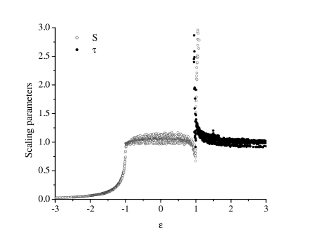
Figure 3: The crossover between two scaling regimes, $\tau\sim 1$ (filled circles) and $S\sim 1$ (empty circles), as energy variable $\varepsilon=(E+2)/V$ changes, is shown for a collection of different values of parameters ($V=0.2-1.2$ and $r_{c}=5-250$) meeting the requirement $\theta\gg 1.$

In the case when the energy $E_{c}$ belongs to the interior of the second spectral region, the scaling properties are determined by the parameter $\kappa$. If $\kappa(E_{c})\ll 1$ we return to the situation of the non-correlated disorder and if $\kappa(E_{c})>1$ the system does not exhibit any scaling behavior in the second spectral region. The destruction of scaling in this case may also be illustrated by the behavior of $\tau(\kappa)$ for different values of $l_{c}$. When $l_{c}$ increases from the values corresponding to the non-correlated limit, the function $\tau(\kappa)$ starts changing as shown in the insert in Fig. 2 where the dependence of $\tau$ is depicted for three different sets of parameters of the random potential $U$ and $r_{c}$. It deviates from the universal (SPS) dependence at larger values of $\kappa$ with the increasing magnitude of the deviation depending upon both $r_{c}$ and $U$. It demonstrates in that way the absence of scaling properties.

IV Conclusion

We considered statistical characteristics and scaling properties of the Lyapunov exponent in a random medium with correlated disorder, using a tight-binding model with a random potential described by a dichotomic process. A simple theoretical approach for estimation of the statistics of the Lyapunov exponent was suggested. Qualitative analysis based on this model allowed us to estimate the effect of correlations on scaling properties, and express this effect in terms of the ratio of the localization length and the correlation length, $\theta=l_{c}/l_{loc}$. When the correlation radius is much smaller than the localization length ($\theta\ll 1$), the system behaves as though correlations are absent and demonstrates single parameter scaling, $\sigma^{2}Ll_{loc}\sim 1,$ whose validity is governed by the ratio $l_{loc}/l_{s}$. In the opposite case, when $\theta\gg 1$, the crossover to another scaling, $\sigma^{2}Ll_{loc}^{2}/l_{c}\sim 1,$ specific for the model under consideration, takes place at values of energy close to the band gap.

References

- (1) E. Abrahams, P. W. Anderson, D. C. Licciardello, and T. V. Ramakrishnan, Phys. Rev. Lett., 42, 673 (1979).
- (2) I. M. Lifshitz, S. A. Gredeskul, L. A. Pastur, Introduction to the theory of disordered systems. (Wiley, NY, 1988).
- (3) D. H. Dunlap, H.-L. Wu, and P. W. Phillips, Phys. Rev. Lett. 65, 88 (1990).
- (4) F. A. B. F. de Moura, M. L. Lyra, Phys. Rev. Lett., 81, 3735 (1998).
- (5) F. M. Izrailev and A. A. Krokhin, Phys. Rev. Lett., 82, 4062 (1999).
- (6) L. Tessieri, cond-mat 0206383, 2002.
- (7) P. W. Anderson, D. J. Thouless, E. Abrahams, and D. S. Fisher, Phys. Rev. B, 22, 3519 (1980).
- (8) A. Cohen, Y. Roth, and B. Shapiro, Phys. Rev. B, 38, 12125 (1988).
- (9) B. Kramer and A. MacKinnon, Localization: theory and experiment, Rep. Prog. Phys. 56, 1469 (1993).
- (10) L. I. Deych, A. A. Lisyansky, and B. L. Altshuler, Phys. Rev. Lett, 84, 2678 (2000); Phys. Rev. B, 64, 224202 (2001).
- (11) L. I. Deych, M. V. Erementchuk, and A.A. Lisyansky, cond-mat 0207169 (2002).
- (12) H. Schomerus, M. Titov, preprint cond-mat/0208457.
- (13) L. Pastur and A. Figotin. Spectra of random and almost-periodic operators. Springer-Verlag, 588 p., 1992.
- (14) J. Avron, W. Craig, and B. Simon, J. Phys. A: Math. Gen., 16, L309 - L311 (1983).
- (15) A. MacKinnon and B. Kramer, Z. Phys. B - Condensed Matter, 53, 1 (1983).