An adaptive smoothing method for traffic state identification from incomplete information

Abstract

We present a new method to obtain spatio-temporal information from aggregated data of stationary traffic detectors, the “adaptive smoothing method”. In essential, a nonlinear spatio-temporal lowpass filter is applied to the input detector data. This filter exploits the fact that, in congested traffic, perturbations travel upstream at a constant speed, while in free traffic, information propagates downstream. As a result, one obtains velocity, flow, or other traffic variables as smooth functions of space and time. Applications include traffic-state visualization, reconstruction of traffic situations from incomplete information, fast identification of traffic breakdowns (e.g., in incident detection), and experimental verification of traffic models.

We apply the adaptive smoothing method to observed congestion patterns on several German freeways. It manages to make sense out of data where conventional visualization techniques fail. By ignoring up to 65% of the detectors and applying the method to the reduced data set, we show that the results are robust. The method works well if the distances between neighbouring detector cross sections do not exceed 3 km.

1 Introduction

During the last decades, traffic dynamics and pedestrian flows have been intensively studied. Regarding the observed phenomena and simulation approaches we refer the reader to some recent reviews [1, 2, 3, 4]. Presently, scientists are more and more getting interested in detailed empirical studies. Reasons for this are the availability of better data and the need to verify and calibrate models. Both, theoretical [5, 6, 7] and empirical [8, 9, 10, 11, 12, 13, 14, 15, 16, 17] studies indicate that the phenomenology of congested traffic is more complex than originally expected. There seems to be a rich spectrum of traffic states [5, 6, 12, 13], hysteretic or continuous temporal or spatial transitions among them [7, 11, 12, 13, 18, 19], and fluctuations or a erratically appearing dynamics play a significant role [13, 16, 20, 21, 22]. In order to make sense out of this, it is increasingly important to have suitable ways of data processing, in order to extract the information relevant for scientific investigations or specific applications. Here, we will propose a three-dimensional data-evaluation method allowing to visualize the spatio-temporal dynamics of traffic patterns along freeways.

The developed “adaptive smoothing method” filters out small-scale fluctuations and adaptively takes into account the main propagation direction of the information flow (i.e. the dominating characteristic line), which have been determined by means of a spatio-temporal correlation analysis in other studies [23]. The temporal length scale of the smoothing procedure can be as small as the sampling interval, while the spatial length scale is related to the distance between successive detectors, which can be up to 3 kilometers long.

By “filter” we just mean a transformation of the data with specific properties. Here, we use a spatio-temporal lowpass filter, i.e., only (Fourier) components of low frequency can pass the filter, while high-frequency contributions are considered as fluctuations and smoothed out. One particular feature of our filter is that it is nonlinear and adaptive to the traffic situation in distinguishing free and congested traffic, as the propagation direction of perturbations differs. The results are three-dimensional visualizations of traffic patterns, which are quite robust with respect to variations of the filter parameters and very helpful in obtaining a clear picture of the systematic spatio-temporal dynamics.

Therefore, this method is suitable for the reconstruction of traffic situations from incomplete information, fast identification of traffic breakdowns (incident detection), and experimental verification of traffic models. First results support the phase diagram of traffic states occuring at bottlenecks [17, 24], which, apart from free traffic, predicts pinned or moving localized clusters, spatially extended patterns such as triggered stop-and-go waves, and oscillating or homogeneous congested traffic, or a spatial coexistence of some of these states [5, 7, 1]. The respectively occuring spatio-temporal pattern depends on the specific freeway flow and bottleneck strength, but also on the level of fluctuations, as these can trigger transitions from, for example, free traffic to localized cluster states [5, 17, 1]. We do not see sufficient support for one “generalized pattern” [25] that would always be observed when traffic flow breaks down.

2 Description of the Method

The adaptive smoothing method is a data processing method for obtaining traffic variables as smooth functions of space and time out of stationary traffic data. It has following heuristically motivated properties:

1. In case of free traffic, perturbations (of, e.g., velocity or flow) move essentially into the direction of traffic flow [26]. More specifically, they propagate with a characteristic velocity $c_{\rm free}$ at about 80% of the desired velocity $V_{0}$ on empty roads [23]. Therefore, at locations with free traffic, perturbations with propagation velocities near $c_{\rm free}$ should pass the filter.

2. In case of congested traffic, perturbations propagate against the direction of traffic flow with a characteristic and remarkably constant velocity $c_{\rm cong}\approx-15$ km [12]. With modern data analysis techniques, it has been shown that such propagation patterns persist even in “synchronized” congested traffic flow, where they are hardly visible in the time series due to a wide scattering of the data in this state [26]. So, for high traffic densities or low velocities, the filter should transmit spatio-temporal perturbations propagating with velocities near $c_{\rm cong}$ more or less unchanged.

3. The filter should smooth out all high-frequency fluctuations in $t$ on a time scale smaller than $\tau$ and spatial fluctuations in $x$ on a length scale smaller than $\sigma$. The parameters $\tau$ and $\sigma$ of the smoothing method can be freely chosen in a wide range (cf. Table 1).

Let us assume that aggregated detector data $\mathchoice{\mbox{\boldmath$\displaystyle z$}}{\mbox{\boldmath$\textstyle z$}}{\mbox{\boldmath$\scriptstyle z$}}{\mbox{\boldmath$\scriptscriptstyle z$}}^{\rm in}_{ij}$ are available from $n$ cross sections $i$ at positions $x_{i}$ where $j\in\{j_{\rm min},\cdots,j_{\rm max}\}$ denotes the index of the aggregation intervals.

Usually, the aggregation interval

$$\Delta t=t_{j}-t_{j-1}$$ (1)

is fixed (between 20 s and 5 min, depending on the measurement device). A typical value for German highways is $\Delta t=1$ min.

The components of $\mathchoice{\mbox{\boldmath$\displaystyle z$}}{\mbox{\boldmath$\textstyle z$}}{\mbox{\boldmath$\scriptstyle z$}}{\mbox{\boldmath$\scriptscriptstyle z$}}^{\rm in}_{ij}$ represent the desired aggregated quantities as obtained from cross section $i$ during the time interval $j$. Typical examples include the average velocity $V_{ij}$, the vehicle flow $Q_{ij}$, the occupancy $O_{ij}$, or some derived quantity such as the traffic density $\rho_{ij}$. The input data $\mathchoice{\mbox{\boldmath$\displaystyle z$}}{\mbox{\boldmath$\textstyle z$}}{\mbox{\boldmath$\scriptstyle z$}}{\mbox{\boldmath$\scriptscriptstyle z$}}^{\rm in}_{ij}$ can represent either averages over all lanes or quantities on a given lane.

The adaptive smoothing method provides estimates $\mathchoice{\mbox{\boldmath$\displaystyle z$}}{\mbox{\boldmath$\textstyle z$}}{\mbox{\boldmath$\scriptstyle z$}}{\mbox{\boldmath$\scriptscriptstyle z$}}(x,t)$ for all locations $x\in[x_{1},x_{n}]$ between the positions of the first and the last detector, and for all times $t\in[t_{\rm min},t_{\rm max}]$. Extrapolations (in the sense of a short-term traffic forecast) will also be discussed. Without loss of generality, we assume $x_{1}<x_{2}<\cdots<x_{n}$, and a traffic flow in positive $x$-direction.

The core of our “adaptive smoothing method” is a nonlinear filter transforming the discrete input detector data $\mathchoice{\mbox{\boldmath$\displaystyle z$}}{\mbox{\boldmath$\textstyle z$}}{\mbox{\boldmath$\scriptstyle z$}}{\mbox{\boldmath$\scriptscriptstyle z$}}_{ij}^{\rm in}$ into the smooth spatio-temporal functions $\mathchoice{\mbox{\boldmath$\displaystyle z$}}{\mbox{\boldmath$\textstyle z$}}{\mbox{\boldmath$\scriptstyle z$}}{\mbox{\boldmath$\scriptscriptstyle z$}}(x,t)$. To satisfy the first two requirements mentioned above, we write the filter as

$$\mathchoice{\mbox{\boldmath$\displaystyle z$}}{\mbox{\boldmath$\textstyle z$}}{\mbox{\boldmath$\scriptstyle z$}}{\mbox{\boldmath$\scriptscriptstyle z$}}(x,t)=w(\mathchoice{\mbox{\boldmath$\displaystyle z$}}{\mbox{\boldmath$\textstyle z$}}{\mbox{\boldmath$\scriptstyle z$}}{\mbox{\boldmath$\scriptscriptstyle z$}}_{\rm cong},\mathchoice{\mbox{\boldmath$\displaystyle z$}}{\mbox{\boldmath$\textstyle z$}}{\mbox{\boldmath$\scriptstyle z$}}{\mbox{\boldmath$\scriptscriptstyle z$}}_{\rm free})\mathchoice{\mbox{\boldmath$\displaystyle z$}}{\mbox{\boldmath$\textstyle z$}}{\mbox{\boldmath$\scriptstyle z$}}{\mbox{\boldmath$\scriptscriptstyle z$}}_{\rm cong}(x,t)+\big{[}1-w(\mathchoice{\mbox{\boldmath$\displaystyle z$}}{\mbox{\boldmath$\textstyle z$}}{\mbox{\boldmath$\scriptstyle z$}}{\mbox{\boldmath$\scriptscriptstyle z$}}_{\rm cong},\mathchoice{\mbox{\boldmath$\displaystyle z$}}{\mbox{\boldmath$\textstyle z$}}{\mbox{\boldmath$\scriptstyle z$}}{\mbox{\boldmath$\scriptscriptstyle z$}}_{\rm free})\big{]}\mathchoice{\mbox{\boldmath$\displaystyle z$}}{\mbox{\boldmath$\textstyle z$}}{\mbox{\boldmath$\scriptstyle z$}}{\mbox{\boldmath$\scriptscriptstyle z$}}_{\rm free}(x,t).$$ (2)

This is a superposition of two linear anisotropic lowpass filters $\mathchoice{\mbox{\boldmath$\displaystyle z$}}{\mbox{\boldmath$\textstyle z$}}{\mbox{\boldmath$\scriptstyle z$}}{\mbox{\boldmath$\scriptscriptstyle z$}}_{\rm cong}(x,t)$ and $\mathchoice{\mbox{\boldmath$\displaystyle z$}}{\mbox{\boldmath$\textstyle z$}}{\mbox{\boldmath$\scriptstyle z$}}{\mbox{\boldmath$\scriptscriptstyle z$}}_{\rm free}(x,t)$ with an adaptive weight factor $0\leq w\leq 1$ which itself depends nonlinearly on the output of the linear filters as discussed later on.

The filter $\mathchoice{\mbox{\boldmath$\displaystyle z$}}{\mbox{\boldmath$\textstyle z$}}{\mbox{\boldmath$\scriptstyle z$}}{\mbox{\boldmath$\scriptscriptstyle z$}}_{\rm cong}(x,t)$ for congested traffic is given by

$$\mathchoice{\mbox{\boldmath$\displaystyle z$}}{\mbox{\boldmath$\textstyle z$}}{\mbox{\boldmath$\scriptstyle z$}}{\mbox{\boldmath$\scriptscriptstyle z$}}_{\rm cong}(x,t)=\frac{1}{N_{\rm cong}(x,t)}\sum\limits_{i=1}^{n}\sum\limits_{j=j_{\rm min}}^{j_{\rm max}}\phi_{\rm cong}(x_{i}-x,t_{j}-t)\mathchoice{\mbox{\boldmath$\displaystyle z$}}{\mbox{\boldmath$\textstyle z$}}{\mbox{\boldmath$\scriptstyle z$}}{\mbox{\boldmath$\scriptscriptstyle z$}}^{\rm in}_{ij},$$ (3)

with

$$t_{j}=t_{\rm min}+j\Delta t,$$ (4)

and the normalization factor

$$N_{\rm cong}(x,t)=\sum\limits_{i=1}^{n}\sum\limits_{j=j_{\rm min}}^{j_{\rm max}}\phi_{\rm cong}(x_{i}-x,t_{j}-t).$$ (5)

This normalization guarantees that a constant input vector $\mathchoice{\mbox{\boldmath$\displaystyle z$}}{\mbox{\boldmath$\textstyle z$}}{\mbox{\boldmath$\scriptstyle z$}}{\mbox{\boldmath$\scriptscriptstyle z$}}^{\rm in}_{ij}=\mathchoice{\mbox{\boldmath$\displaystyle z$}}{\mbox{\boldmath$\textstyle z$}}{\mbox{\boldmath$\scriptstyle z$}}{\mbox{\boldmath$\scriptscriptstyle z$}}_{0}$ for all $i,j$ is transformed into a constant output function with the same components: $\mathchoice{\mbox{\boldmath$\displaystyle z$}}{\mbox{\boldmath$\textstyle z$}}{\mbox{\boldmath$\scriptstyle z$}}{\mbox{\boldmath$\scriptscriptstyle z$}}(x,t)=\mathchoice{\mbox{\boldmath$\displaystyle z$}}{\mbox{\boldmath$\textstyle z$}}{\mbox{\boldmath$\scriptstyle z$}}{\mbox{\boldmath$\scriptscriptstyle z$}}_{0}$. Notice that the normalization depends on both, location $x$ and time $t$.

The analogous expression for the lowpass filter $\mathchoice{\mbox{\boldmath$\displaystyle z$}}{\mbox{\boldmath$\textstyle z$}}{\mbox{\boldmath$\scriptstyle z$}}{\mbox{\boldmath$\scriptscriptstyle z$}}_{\rm free}(x,t)$ for free traffic is

$$\mathchoice{\mbox{\boldmath$\displaystyle z$}}{\mbox{\boldmath$\textstyle z$}}{\mbox{\boldmath$\scriptstyle z$}}{\mbox{\boldmath$\scriptscriptstyle z$}}_{\rm free}(x,t)=\frac{1}{N_{\rm free}(x,t)}\sum\limits_{i=1}^{n}\sum\limits_{j=j_{\rm min}}^{j_{\rm max}}\phi_{\rm free}(x_{i}-x,t_{j}-t)\mathchoice{\mbox{\boldmath$\displaystyle z$}}{\mbox{\boldmath$\textstyle z$}}{\mbox{\boldmath$\scriptstyle z$}}{\mbox{\boldmath$\scriptscriptstyle z$}}^{\rm in}_{ij}$$ (6)

with

$$N_{\rm free}(x,t)=\sum\limits_{i=1}^{n}\sum\limits_{j=j_{\rm min}}^{j_{\rm max}}\phi_{\rm free}(x_{i}-x,t_{j}-t).$$ (7)

Figure 1: Visualization of the effects of linear homogeneous filters with the kernels $\phi_{\rm free}(x,t)$ and $\phi_{\rm cong}(x,t)$, respectively. The shaded areas denote the regions considered in the calculation of a data point at $(x,t)$. Triangles denote the mainly contributing input data sampled in free traffic, squares the ones sampled in congested traffic.

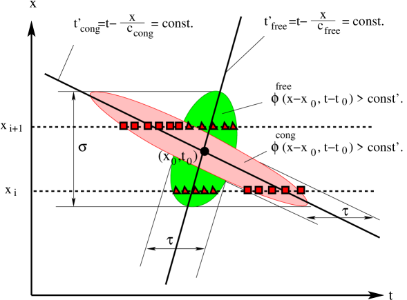
The kernels $\phi_{\rm cong}(x,t)$ and $\phi_{\rm free}(x,t)$ of the linear homogeneous filters do the required smoothing and are particularly transmissible for perturbations propagating with the typical velocities $c_{\rm cong}$ and $c_{\rm free}$ observed in congested and free traffic, respectively (cf. Fig. 1).

If the propagation velocity of the perturbations was zero, the filter should only perform the smoothing. We chose the (non-normalized) exponential function

$$\phi_{0}(x,t)=\exp\left(-\frac{|x|}{\sigma}-\frac{|t|}{\tau}\right).$$ (8)

Instead, one could apply other localized functions such as a two-dimensional Gaussian. However, it turned out that the exponential had more favourable properties in our application.

The linear filter for nonzero propagation velocities can be mapped to $\phi_{0}(x,t)$ by the coordinate transformations (cf. Fig. 1)

$$x=x^{\prime},\ \ \ t=t^{\prime}_{\rm cong}+\frac{x}{c_{\rm cong}}=t^{\prime}_{\rm free}+\frac{x}{c_{\rm free}}.$$ (9)

Thus, we obtain for the kernels of the linear anisotropic filters

$$\phi_{\rm cong}(x,t) = \phi_{0}(x^{\prime},t^{\prime}_{\rm cong})=\phi_{0}\left(x,t-\frac{x}{c_{\rm cong}}\right),$$ (10)

$$\phi_{\rm free}(x,t) = \phi_{0}(x^{\prime},t^{\prime}_{\rm free})=\phi_{0}\left(x,t-\frac{x}{c_{\rm free}}\right).$$ (11)

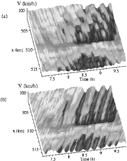
Figure 2 shows the action of the filters $\mathchoice{\mbox{\boldmath$\displaystyle z$}}{\mbox{\boldmath$\textstyle z$}}{\mbox{\boldmath$\scriptstyle z$}}{\mbox{\boldmath$\scriptscriptstyle z$}}_{\rm cong}(x,t)$ and $\mathchoice{\mbox{\boldmath$\displaystyle z$}}{\mbox{\boldmath$\textstyle z$}}{\mbox{\boldmath$\scriptstyle z$}}{\mbox{\boldmath$\scriptscriptstyle z$}}_{\rm free}(x,t)$ for the velocity fields $V_{\rm cong}(x,t)$ and $V_{\rm free}(x,t)$.

Figure 2: Typical velocity fields $V_{\rm free}(x,t)$ (top) and $V_{\rm cong}(x,t)$ (bottom) obtained by application of the filters $\mathchoice{\mbox{\boldmath$\displaystyle z$}}{\mbox{\boldmath$\textstyle z$}}{\mbox{\boldmath$\scriptstyle z$}}{\mbox{\boldmath$\scriptscriptstyle z$}}_{\rm free}(x,t)$ and $\mathchoice{\mbox{\boldmath$\displaystyle z$}}{\mbox{\boldmath$\textstyle z$}}{\mbox{\boldmath$\scriptstyle z$}}{\mbox{\boldmath$\scriptscriptstyle z$}}_{\rm cong}(x,t)$ to traffic data of a section of the German freeway A9 South.

Finally, we define the nonlinear adaptive weight function $w(\mathchoice{\mbox{\boldmath$\displaystyle z$}}{\mbox{\boldmath$\textstyle z$}}{\mbox{\boldmath$\scriptstyle z$}}{\mbox{\boldmath$\scriptscriptstyle z$}}_{\rm cong},\mathchoice{\mbox{\boldmath$\displaystyle z$}}{\mbox{\boldmath$\textstyle z$}}{\mbox{\boldmath$\scriptstyle z$}}{\mbox{\boldmath$\scriptscriptstyle z$}}_{\rm free})\in[0,1]$. Obviously, we must have $w\approx 1$ for congested traffic, and $w\approx 0$ for free traffic, so we need some a priori estimate of the traffic situation at the point $(x,t)$.

Congested traffic is characterized by a high traffic density and low average velocity. Since, in contrast to the density, the velocity can be directly measured with stationary detectors, we chose the velocity to determine the a priori estimate. Different possibilities to estimate the velocity at point $(x,t)$ are:

• The measured velocity $V_{ij}$ of the detector cross section whose position $x_{i}$ is nearest to $x$ in the time interval $j$ containing the actual time $t$,

• the velocity $V_{\rm cong}(x,t)$ as calculated with the “congested-traffic” filter $\mathchoice{\mbox{\boldmath$\displaystyle z$}}{\mbox{\boldmath$\textstyle z$}}{\mbox{\boldmath$\scriptstyle z$}}{\mbox{\boldmath$\scriptscriptstyle z$}}_{\rm cong}$ according to Eq. (3) with kernel (10) (assuming a priori congested traffic),

• the velocity $V_{\rm free}(x,t)$ as calculated with the “free-traffic” filter $\mathchoice{\mbox{\boldmath$\displaystyle z$}}{\mbox{\boldmath$\textstyle z$}}{\mbox{\boldmath$\scriptstyle z$}}{\mbox{\boldmath$\scriptscriptstyle z$}}_{\rm free}$ according to Eq. (6) with the kernel (11),

• or some combination of the above estimates.

The first way to estimate the velocity is subject to errors, if the typical length scale $\lambda$ of occuring stop-and-go structures is not larger than the distance $\Delta x_{i}$ between two neighbouring detectors. At this point, it is crucial that propagating structures in congested traffic, especially stop-and-go waves, are very persistent. It has been shown [27] that they can propagate through freeway intersections or other inhomogeneities nearly unchanged, passing all perturbations of free traffic on their way (see, e.g., Fig. 9). Therefore, whenever at least one of the estimates indicates congested traffic, the weight function should favour the filter for congested traffic. Specifically, we assume

$$w(\mathchoice{\mbox{\boldmath$\displaystyle z$}}{\mbox{\boldmath$\textstyle z$}}{\mbox{\boldmath$\scriptstyle z$}}{\mbox{\boldmath$\scriptscriptstyle z$}}_{\rm cong},\mathchoice{\mbox{\boldmath$\displaystyle z$}}{\mbox{\boldmath$\textstyle z$}}{\mbox{\boldmath$\scriptstyle z$}}{\mbox{\boldmath$\scriptscriptstyle z$}}_{\rm free})=w(V_{\rm cong}(x,t),V_{\rm free}(x,t))=\frac{1}{2}\left[1+\tanh\left(\frac{V_{c}-V^{*}(x,t)}{\Delta V}\right)\right]\,,$$ (12)

where

$$V^{*}(x,t)=\min\bigg{(}V_{\rm cong}(x,t),V_{\rm free}(x,t)\bigg{)}\,.$$ (13)

$V_{c}$ and $\Delta V$ are parameters that can be varied in a wide range.

If not explicitely stated otherwise, for all simulations in the following section we will use the parameters specified in Table 1. We will also show that the four parameters $c_{\rm cong}$, $c_{\rm free}$, $V_{c}$ and $\Delta v$ can be varied in a wide range without great differences in the output. In this way, we show that the proposed adaptive smoothing method does not need to be calibrated to the respective freeway. One can take the values from Table 1 as a global setting.

The smoothing parameters $\sigma$ and $\tau$ have the same meaning and the same effect as in standard smoothing methods, e.g., Eqs. (22) and (23) in Ref. [17].

Parameter	Typical Value	Meaning
$\sigma$	0.6 km	Range of spatial smoothing in $x$
$\tau$	1.1 min	Range of temporal smoothing in $t$
$c_{\rm free}$	80 km/h	Propagation velocity of perturbations in free traffic
$c_{\rm cong}$	$-15$ km/h	Propagation velocity of perturbations in congested traffic
$V_{c}$	60 km/h	Crossover from free to congested traffic
$\Delta V$	20 km/h	Width of the transition region

Table 1: Parameters of the “adaptive smoothing method” defined by Eqs. (2)–(13), their interpretation, and their typical values.

In summary, the proposed “adaptive smoothing method” is given by Eq. (2) with the nonlinear weight function (12), the filter (3) with normalization (5) and kernel (10) for congested traffic, the filter (6) with normalization (7) and kernel (11) for free traffic, and the smoothing filter (8). Table 1 gives an overview of the six parameters involved and typical values for them. The adaptive smoothing method includes the following special cases:

• Isotropic smoothing resulting in the limits $c_{\rm free}\to\infty$ and $c_{\rm cong}\to\infty$ (for practical purposes, one may chose $c_{\rm free}=c_{\rm cong}=10^{6}$ km/h);

• only filtering for structures of congested traffic in the limit $V_{c}\to\infty$ (for practical purposes, one may set $V_{c}\gg V_{0}$ with $V_{0}$ being the desired velocity);

• only filtering for structures of free traffic for $V_{c}=\Delta V=0$;

• consideration of the data of the nearest detector only, if $\sigma=0$;

• application of the actual sampling interval of the detectors, if $\tau=0$, $c_{\rm free}\to\infty$ and $c_{\rm cong}\to\infty$. (To avoid divisions by zero, zero values of $\sigma$, $\tau$, and $\Delta V$ are replaced by very small positive values in the software).

3 Application to German Freeways

We will now discuss data from the German freeways A8-East and A9-South near Munich, and of the freeway A5-North near Frankfurt. In all cases, the traffic data were obtained from several sets of double-induction-loop detectors recording, separately for each lane, the passage times and velocities of all vehicles. Only aggregate information was stored with an aggregation interval of $\Delta t=1$ min. We will use the following input data $\mathchoice{\mbox{\boldmath$\displaystyle z$}}{\mbox{\boldmath$\textstyle z$}}{\mbox{\boldmath$\scriptstyle z$}}{\mbox{\boldmath$\scriptscriptstyle z$}}_{ij}^{\rm in}$:

• The lane-averaged vehicle flow

  $$Q_{ij}=\sum_{l=1}^{L}\frac{n_{ij}^{l}}{L\Delta t}\,,$$ (14)

  where $n_{ij}^{l}$ is the vehicle count at cross section $i$ during time interval $j$ on lane $l$. The considered sections of the freeways have $L=3$ lanes in most cases.

• The lane-averaged mean velocity

  $$V_{ij}=\sum_{l=1}^{L}\frac{Q_{ij}^{l}V_{ij}^{l}}{Q_{ij}}\,,$$ (15)

  where $V_{ij}^{l}$ is the average velocity at cross section $i$ during time interval $j$ on lane $l$.

• The traffic density determined via the formula

  $$\rho_{ij}=\frac{Q_{ij}}{V_{ij}}\,,$$ (16)

  as occupancies were not available for all freeways.

Figure 3: Complex congested traffic pattern on the German freeway A8-East from Munich to Salzburg during the evening rush hour on November 2, 1998. (a) Sketch of the freeway. (b) Plot of the spatio-temporal density $\rho(x,t)$ using conventional smoothing (resulting for the setting $c_{\rm free}=c_{\rm cong}=10^{6}$ km/h). (c) Plot of the same data as calculated with the adaptive smoothing method.

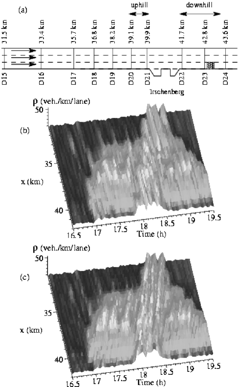
Figure 3 shows an example of a complex traffic breakdown that occurred on the freeway A8 East from Munich to Salzburg during the evening rush hour on November 2, 1998. Two different kinds of bottlenecks were relevant, (i) a relatively steep uphill gradient from $x=38$ km to $x=40$ km (the “Irschenberg”), and (ii) an incident leading to the closing of one of the three lanes between the cross sections D23 and D24 between $t=$ 17:40 h and $t=$ 18:10 h. For further details, see Ref. [17]. Figure 3(c) shows the traffic density using the proposed data processing method with the parameters specified in Table 1. For comparison, (b) shows the result of conventional isotropic smoothing ignoring the speed of information propagation, cf. Ref. [17]. While the structures in the free-traffic regions are nearly the same in both plots, the new smoothing method gives a better reconstruction of the congested traffic patterns. In contrast to the conventional method, our proposed method can resolve oscillations with wavelengths $\lambda$ comparable to or smaller than the distance $\Delta x_{i}$ between two neighbouring cross sections as illustrated for the three stop-and-go waves propagating through the whole displayed section ($\lambda\approx 2$ km). Notice that the conventional method generates artefacts for this example.

The congestion patterns caused by the uphill gradient (the “wings” in Fig. 3(b), (c)) have larger characteristic wavelengths and are resolved, at least partially, also with the conventional method.

Figure 4: Time series of the empirical density, approximated by means of Eq. (16), for several cross sections.

Figure 5: Time series of the empirical velocity data determined via Eq. (15) for cross section D20.

For comparison, we plot time series of some cross sections in Figure 4. Let us consider more closely the jammed traffic patterns caused by the temporary bottleneck associated with the incident. While the fluctuations are irregular at detector D22 (about 1.2 km upstream of the aforementioned incident), they grow to three stop-and-go waves further upstream, cf. the arrows in Fig. 5. However, due to measurement errors and other errors in determining the density [1], the time series of the density is very noisy, especially that of cross section D20. The adaptive smoothing method suppresses this noise without suppressing the structure of the pattern.

To check, whether there are significant patterns in the data of detector D20 at all, we plot the velocity data at D20 as well (Fig. 5). In contrast to the density, the velocity is measured directly resulting in less noise. One clearly sees three dips corresponding to three stop-and-go waves which confirms the results of the “adaptive smoothing method”.

Figure 6: Spatio-temporal density $\rho(x,t)$ as in Figure 3, but using only the data of cross sections D16, D18, D20, and D22 as input (cf. Figure 4).

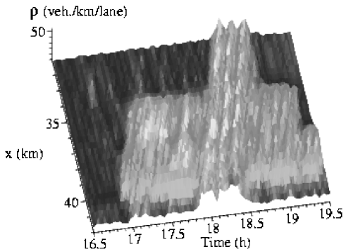
As a further check that the structures shown in Fig. 3(c) are not artefacts of the data processing, we tested the method for a reduced data set. Figure 6 shows the result using only the even-numbered detectors as input, whose time series are plotted in Fig. 4. The main structures remain nearly unchanged, particularly, the three stop-and-go waves propagating through the whole section. Notice that the whole plot is based on data of only four cross sections, and that the data are extrapolated in the upstream direction over a distance of nearly 2 km.

Figure 7: Two regions of stop-and-go waves on the German freeway A9-South near Munich occurring upstream of the freeway intersections I1 and I2. (a) Sketch of the freeway. (b) Plot of the inverse $1/V(x,t)$ of the spatio-temporal velocity $V(x,t)$, using conventional smoothing. (c) Plot of the same data using the adaptive smoothing method.

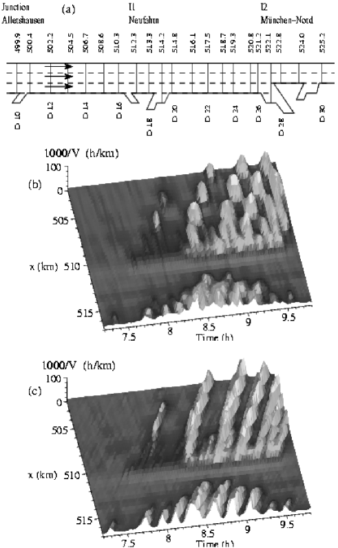
We now apply the processing method to data from a section of the freeway A9-South near Munich. There are two major intersections I1 and I2 with other freeways. Virtually every weekday, traffic broke down to oscillatory congested traffic upstream of each of these intersections. (For details, see Ref. [17]).

Figure 7 (b) shows the inverse of the velocity, $1/V(x,t)$ for a typical congested situation. When plotting $1/V(x,t)$, the structures of congested traffic comes out more clearly than for the density. The method resolves small density clusters in the region 508 km $\leq x\leq 510$ km between about 8:30 am and 9:30 am which disappear around $x=508$ km. These structures cannot be identified with the conventional smoothing method (see Fig. 7(c)), which just shows a hilly pattern.

Figure 7(b) is an example for the spatial coexistence of homogeneous congested traffic (a short stretch around $x=510$ km), oscillating congested traffic (around $x=509$ km), and stop-and-go waves (around $x=507$ km). This may be a three-dimensional illustration of the so-called “pinch effect” [11, 14], but we do not observe a merging of narrow clusters to form wide moving jams. The narrow structures of short wavelengths rather disappear. This may be an artefact of our smoothing method, so that video data are required to get a more detailed picture. Simulations of this spatial coexistence, however, indicate that narrow clusters rather disappear than merge, namely when they do not exceed the critical amplitude in an area of metastable traffic [7].

Notice that the bottleneck causing this congestion is located at about $x=510$ km implying that it is caused by weaving traffic and slowing down at an off-ramp, not by an on-ramp as is most often the case on German highways.

Figure 8: Same data and same processing method as in Figure 7(c), but with (a) a propagation velocity of $c_{\rm cong}=-12$ km/h instead of -15 km/h (b) $c_{\rm cong}=-20$ km/h, (c) with the crossover parameter $V_{c}=40$ km/h instead of 60 km/h.

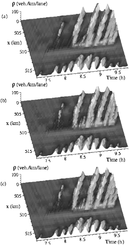
Now we demonstrate that the method is robust with respect to reasonable parameter changes. Figure 8(a) shows the result for an assumed propagation velocity of $c_{\rm cong}=-12$ km/h instead of -15 km/h. In plot (b), we assumed $c_{\rm cong}=-20$ km/h instead. In both cases, the results are systematically better than with the isotropic procedure. Since the propagation velocity of perturbations in congested traffic is always about $c_{\rm cong}=-15$ km [12, 23, 28, 29], one can take this value as a global setting.

Due to the comparatively high magnitude of the propagation velocity $c_{\rm free}$, the related time shifts in the transformation (9) for free traffic are small. Therefore, the method is insensitive to changes with respect to this parameter. It turned out that taking the isotropic limit $c_{\rm free}\to\infty$ nearly gives the same results.

The crossover parameters $V_{c}$ and $\Delta V$ can be varied within reasonable limits as well. As an example, Fig. 8(c) shows the result after changing the crossover velocity from $V_{c}=60$ km/h to $V_{c}=40$ km/h.

Figure 9: Freeway A5-North from Frankfurt to Kassel during the evening rush hour on August 7, 1998. (a) Sketch of the freeway. (b) Data reconstruction of the velocity using all detectors D10–D26. (c) Reconstruction using a reduced data set of only 6 of all 17 detectors used in (b).

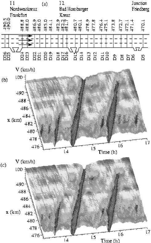
Finally, we applied the method to isolated moving localized clusters and pinned localized clusters observed on the A5-North near Frankfurt. This freeway is particularly well equipped with detectors, so that the typical length scales of the observed structures are always larger than the distance between neighbouring detectors. However, we obtained nearly the same results when using only the even-numbered detectors or only the odd-numbered detectors as input. Figure 9 shows that even a further reduction of the information to only 35% of the detectors yields good results.

4 Summary and Outlook

We have proposed a new “adaptive smoothing method” for the three-dimensional visualization of spatio-temporal traffic patterns, which takes into account the characteristic propagation velocities observed in free and congested traffic. The method is robust with respect to variations of its parameters, so that it can be applied to new freeway sections without calibration. In principle, it would be possible to determine the parameters (such as the propagation velocity of perturbations) locally (e.g., by means of a correlation analysis). However, the results would look less smooth and regular, as the small number of data to determine the local parameters would be associated with considerable statistical errors. Consequently, a large part of the variations in the local parameters would not reflect systematic variations of the parameters. So, both the local and global parameter calibration may produce artefacts, but it is advantageous to use global parameter settings. Moreover, there is empirical support for surprisingly constant propagation velocities $c_{\rm free}$ and $c_{\rm cong}$ of perturbations in free and congested traffic. The parameters $V_{c}$ and $\Delta V$ are related to the transition from free to congested traffic and, therefore, can also be well determined. The spatial and temporal smoothing parameters $\sigma$ and $\tau$ can be specified according to the respective requirements. Suitable parameters allow a good representation of traffic patterns even when the distances between successive detectors are about 3 kilometers.

We point out that the suggested “adaptive smoothing method” itself can be applied to calibrate the characteristic propagation velocities $c_{\rm free}$ and $c_{\rm cong}$. For this purpose, the ranges $\sigma$ and $\tau$ of spatial and temporal smoothing are chosen small. The optimal propagation velocities minimize the offsets in the propagation patterns.

The aim of the “adaptive smoothing method” is to reconstruct the spatio-temporal traffic data from incomplete information as good as possible to allow a better understanding of the complex traffic dynamics. Potential applications are, for example, traffic state visualization, incident detection, or the experimental verification of traffic models. Our method could be further improved by taking into account information about the traffic dynamics such as the continuity equation or a suitable equation for the average vehicle velocity as a function of space and time. It could, then, be used to determine short-term traffic forecasts.

Acknowledgments

The authors would like to thank the German Research Foundation (DFG) for financial support through the grant He 2789/2-1. They are also grateful to the Autobahndirektion Südbayern, and the Hessisches Landesamt für Straßen und Verkehrswesen for providing the traffic data.

References

- [1] D. Helbing, Traffic and related self-driven many-particle systems, Reviews of Modern Physics 73, 1067–1141 (2001).
- [2] D. Chowdhury, L. Santen, and A. Schadschneider, Statistical physics of vehicular traffic and some related systems, Physics Reports 329, 199–329 (2000).
- [3] D. Helbing, I. J. Farkas, P. Molnár, and T. Vicsek, Simulation of pedestrian crowds in normal and evacuation situations, in Pedestrian and Evacuation Dynamics, edited by M. Schreckenberg and S. D. Sharma (Springer, Berlin, 2002), pp. 21–58.
- [4] D. Helbing, P. Molnár, I. Farkas, and K. Bolay, Self-organizing pedestrian movement, Environment and Planning B 28, 361–383 (2001).
- [5] D. Helbing, A. Hennecke, and M. Treiber, Phase diagram of traffic states in the presence of inhomogeneities, Phys. Rev. Lett. 82, 4360–4363 (1999).
- [6] H. Y. Lee, H.-W. Lee, and D. Kim, Dynamic states of a continuum traffic equation with on-ramp, Phys. Rev. E 59, 5101–5111 (1999).
- [7] M. Treiber and D. Helbing, Explanation of observed features of self-organization in traffic flow, e-print cond-mat/9901239 (1999).
- [8] M. J. Cassidy and R. L. Bertini, Some traffic features at freeway bottlenecks, Transpn. Res. B 33, 25–42 (1999).
- [9] C. F. Daganzo, M. J. Cassidy, and R. L. Bertini, Possible explanations of phase transitions in highway traffic, Transpn. Res. A 33, 365–379 (1999).
- [10] F. L. Hall and K. Agyemang-Duah, Freeway capacity drop and the definition of capacity, Transpn. Res. Rec. 1320, 91–108 (1991).
- [11] B. S. Kerner, Experimental features of self-organization in traffic flow, Phys. Rev. Lett. 81, 3797–3800 (1998).
- [12] B. S. Kerner and H. Rehborn, Experimental features and characteristics of traffic jams, Phys. Rev. E 53, R1297–R1300 (1996).
- [13] B. S. Kerner and H. Rehborn, Experimental properties of complexity in traffic flow, Phys. Rev. E 53, R4275–R4278 (1996).
- [14] M. Koshi, M. Iwasaki, and I. Ohkura, Some findings and an overview on vehicular flow characteristics, in Proceedings of the 8th International Symposium on Transportation and Traffic Flow Theory, pp. 403–426, V. F. Hurdle, E. Hauer, and G. N. Stewart (Eds.) (University of Toronto, Toronto, Ontario, 1983).
- [15] H. Y. Lee, H.-W. Lee, and D. Kim, Phase diagram of congested traffic flow: An empirical study, Phys. Rev. E 62, 4737–4741 (2000).
- [16] L. Neubert, L. Santen, A. Schadschneider, and M. Schreckenberg, Single-vehicle data of highway traffic: A statistical analysis, Phys. Rev. E 60, 6480–6490 (1999).
- [17] M. Treiber, A. Hennecke, and D. Helbing, Congested traffic states in empirical observations and microscopic simulations, Phys. Rev. E 62, 1805–1824 (2000).
- [18] D. Helbing and M. Treiber, Gas-kinetic-based traffic model explaining observed hysteretic phase transition, Phys. Rev. Lett. 81, 3042–3045 (1998).
- [19] H. Y. Lee, H.-W. Lee, and D. Kim, Origin of synchronized traffic flow on highways and its dynamic phase transitions, Phys. Rev. Lett. 81, 1130–1133 (1998).
- [20] J. H. Banks, An investigation of some characteristics of congested flow, Transpn. Res. Rec. 1678, 128–134 (1999).
- [21] W. Leutzbach, Introduction to the Theory of Traffic Flow (Springer, Berlin, 1988).
- [22] M. Treiber and D. Helbing, Macroscopic simulation of widely scattered synchronized traffic states, J. Phys. A: Math. Gen. 32, L17–L23 (1999).
- [23] R. Sollacher, B. S. Kerner, P. Konhäuser, H. Rehborn, R. Kühne, M. Schreckenberg, and D. Helbing, SANDY - Nichtlineare Dynamik im Straßenverkehr, in Technische Anwendungen von Erkenntnissen der Nichtlinearen Dynamik (VDI - Technologiezentrum Physikalische Technologien, Düsseldorf, ISBN 3-931384-25-X, 1999).
- [24] D. Helbing and M. Treiber, Critical discussion of “sychronized flow”, submitted to Cooper@tive Tr@nsport@tion Dyn@mics (2002).
- [25] B. S. Kerner and S. L. Klenov, A micropscopic model for phase transitions in traffic flow, J. Phys. A: Math. Gen. 35, L31–L43 (2002).
- [26] C. F. Daganzo, A behavioral theory of multi-lane traffic flow, Part I: Long homogeneous freeway sections, (ITS Working Paper, UCB-ITS-RR-99-5, revised June 20, 2000).
- [27] B. S. Kerner, Theory of breakdown phenomenon at highway bottlenecks, Transpn. Res. Rec. 1710, 136–144 (2000).
- [28] M. J. Cassidy and M. Mauch, An observed traffic pattern in long freeway queues, Transpn. Res. A 35, 143–156 (2001).
- [29] H. S. Mika, J. B. Kreer, and L. S. Yuan, Dual mode behavior of freeway traffic, Highw. Res. Rec. 279, 1–13 (1969).