Cooling non–linear lattices toward energy localisation
Abstract
We describe the energy relaxation process produced by surface damping on lattices of classical anharmonic oscillators. Spontaneous emergence of localised vibrations dramatically slows down dissipation and gives rise to quasi-stationary states where energy is trapped in the form of a gas of weakly interacting discrete breathers. In one dimension (1D), strong enough on–site coupling may yield stretched–exponential relaxation which is reminiscent of glassy dynamics. We illustrate the mechanism generating localised structures and discuss the crucial role of the boundary conditions. For two–dimensional (2D) lattices, the existence of a gap in the breather spectrum causes the localisation process to become activated. A statistical analysis of the resulting quasi-stationary state through the distribution of breathers’ energies yield information on their effective interactions.
pacs:
63.20.Ry, 63.20.PwDiscrete breathers have been widely analysed as mathematical objects, but the relevance of their role in physical systems is still debated. In fact, any mechanism yielding the spontaneous formation of breathers is expected to provide interesting indications in this direction. In this respect, the phenomenon of relaxation to breather states by cooling lattices from their boundaries is one of the most interesting examples. Here we provide a comprehensive description of this phenomenon in low dimensional lattices. In particular, we review former results and add new information, mainly concerning the 2D case. This study is based on a combination of numerics and theoretical arguments, while we analyse both dynamical and statistical features of the problem to clarify the whole scenario.
I Introduction
Nonlinearity has revealed one of the key ingredients for describing many relevant features of different states of matter. In the realm of lattice dynamics, scattering processes among phonons, propagation of solitary waves and slow energy relaxation are typical examples. Recently, considerable efforts have been devoted to the study of periodic, localised, non–linear lattice excitations, named ”breathers” breath1 . They are quite peculiar (but generic) objects emerging from the interplay of nonlinearity and space discreteness breath2 . Their mathematical properties, like existence, stability, mobility etc. have been progressively unveiled, while they have been identified in many different scenarios.
Their role in non–equilibrium dynamics seems to be particularly fascinating. An example is the relaxation to energy equipartition of short–wavelength fluctuations chao_breath . Another interesting scenario where breathers are found to emerge spontaneously is observed upon cooling the lattice at its boundaries Aubry1 ; Aubry2 ; noi , i.e. by considering a non–equilibrium process in which energy exchange with the environment is much faster at the surface than in the bulk. The numerical simulations neatly show that the energy dissipation rate may be significantly affected by the spontaneous excitation of breathers. As the latter exhibit a very weak interaction among themselves and with the boundaries, the energy release undergoes a sudden slowing down and is hardly detected on the time scales of a typical simulation. Thus, the lattice remains frozen in a pseudo–stationary, metastable configuration which is far from thermal equilibrium, which we shall refer to as residual state. Despite the absence of disorder, there is a close similarity with the glassy behaviour observed in disordered systems, as was already pointed out Aubry1 ; Aubry2 .
But what are the mechanisms leading to spontaneous localisation? As we have shown in a previous paper noi , the latter is intimately related to how dissipation acts on vibrational modes of different wavelengths. If long–wavelength phonons can be efficiently damped out, the modulation instability of short lattice waves Peyrard becomes highly favoured and breathers can easily emerge from an interacting soliton–gas chao_breath ; Kosevich . In this respect, this type of non–equilibrium condition is much more effective in exciting localised modes than an equilibrium one (see e.g. Bishop for a related discussion).
Spontaneous localisation upon cooling has been observed for both on–site Aubry1 ; Aubry2 and pure nearest–neighbour (n.n.) interactions noi ; reigada1 . The two classes of models are known to behave differently, e.g. as to the mobility of breathers, which is much higher in the absence of local coupling. This is also confirmed by relaxations experiments, where differences in the energy decay laws have been observed. In particular, the approach to the residual state follows a simple exponential law in the Fermi-Pasta-Ulam (FPU) system noi , but turns to stretched exponential in the presence of local coupling Aubry2 .
Our aim in this paper is to provide an up–to–date overview of the phenomenon of breather localisation by cooling. Generalities about the energy release process, including models and indicators, will be presented in Section II, along with the discussion of the cooling process in an harmonic lattice and the results obtained for 1D non–linear systems. In particular we shall survey the different cooling pathways appearing in pure n.n. and on–site potentials. A specific subsection will be devoted to clarify the interpretation of some recent results reigada1 ; reigada2 . In Section III, we present the results for the n.n. 2D FPU model. We want to point out that the 2D is not a straightforward extension of the 1D case. Indeed, the existence of an energy activation threshold for breather solutions 2D_tresh leads to conjecture that a thermalised state may be cooled to the residual state only above some initial energy/temperature. Moreover, the residual state is a static multi–breather state, whereby in the 1D case it usually contains a single breather. Finally, we perform an analysis of the distribution of breather energies, based on a simple statistical model.
II Relaxation and localisation in 1D
In this section we will describe the lattice models and the generalities of a typical relaxation experiment as well as the relevant indicators used throughout the paper. Let us consider a chain of atoms of unit mass and denote with the displacement of the –th particle from its equilibrium position ( is the lattice spacing). The atoms are labelled by the index and their dynamics is given by the equations of motion
where and are the interparticle and on–site potentials, respectively. We assume that , denoting with a prime the derivative with respect to . For convenience, we shall adopt non–dimensional units such that and are set to unity. Moreover, as we want to deal with systems in a finite volume, we will impose either free–end (, ) or fixed–end () boundary conditions (BC).
The last term in eq. (II) represents the interaction of the atoms with a “zero–temperature” heat bath in the form of a linear damping with rate . Following Aubry1 ; Aubry2 , we restricted to the case in which dissipation selectively acts only on the atoms located at the chain edges. As mentioned above, this choice is crucial and should model a physical situation in which energy exchange with the environment is much faster at the surface than in the bulk.
The general layout of a simulation can be summarised as follows . First, an equilibrium microstate is generated by, say, Nosè-Hoover (canonical) method Aubry1 or by letting the Hamiltonian (microcanonical) system ( = 0) evolve for a sufficiently long transient noi . In the following we will follow the second strategy. The initial condition for the transient is assigned by setting all displacements to zero and by drawing velocities at random from a Gaussian distribution. The velocities are then rescaled by a suitable factor to fix the desired value of the energy density (energy per particle) . The resulting set of and is then used as initial condition to integrate Eqs. (II) with (see again Ref. noi for details).
The result of the relaxation process is the residual state, i.e. a state with a finite fraction of the initial energy stored in the form of breathers. Remarkably, such residual state is characterised by a decay time scale which is several orders of magnitude longer than that of the localisation process.
II.1 The harmonic lattice
A number of features which characterise the relaxation dynamics of non–linear lattices can be better understood by first studying the harmonic lattice, namely
We anticipate that the presence of an harmonic on–site potential does not alter the main conclusions. We thus take throughout this section.
For small damping, an approximate analytical solution can be found by time–dependent perturbation theory. Let and () denote the eigenvalues and normalized eigenvectors of the unperturbed Hamiltonian problem, where the allowed wave–numbers are and for free–end and fixed–end BC, respectively. To the lowest order in one obtains noi
| (1) |
where is the -th component of the eigenvector and are constant amplitudes fixed by the initial conditions. Notice that, since the number of the damped particles is fixed, the perturbative approximation is expected to improve upon increasing the system size . The wavenumber-dependent damping rates are found to be
| (2) |
with . The free–end and fixed–end BC systems thus show considerably different behaviours. In the former case, the least damped modes are the short–wavelength ones (), the largest lifetime being , while the most damped modes are the ones in the vicinity of , with being the shortest decay time. On the contrary, for fixed ends the most damped modes are those around the band center () while short– and long–wavelength ones dissipate very weakly, being . As we shall illustrate in the following, such difference is crucial for the localisation in the non–linear system.
Using the solution (1), we evaluated the chain energy in the case of equipartition i.e. by replacing with its average value . Finally, recalling eqs. (2) and approximating for large the sum over with an integral (), we obtained noi
| (3) |
where is the modified zero–order Bessel function, whose asymptotic expansions have been used to obtain the last equality. We conclude that relaxation is exponential only at short times while a crossover to a power–law decay occurs at . Moreover, despite the differences in the relaxation times (2), the decay law for turns out to be the same in the free and fixed–end systems.
The above formulas must be taken with caution when dealing with a large but finite system. In such a case, there is of course a lower cutoff at wavenumbers of order . Therefore, after a time of the order of the lifetime of the longest–lived mode, , formula (3) no longer holds and a further crossover to the exponential decay law occurs. This has been also verified numerically noi .
II.2 Non–linear lattices: the role of discreteness
Since the first results of relaxation experiments in non–linear lattices were reported Aubry1 ; Aubry2 , there has been some debate as to the nature of the decay law of the system energy and its relation with the spontaneously emerging localised modes. In particular, it has been claimed that the phenomenon of energy pinning in the form of discrete breathers would result in a glassy–like relaxation, i.e. stretched exponential decay law. Here we shall describe how the main role in determining the relaxation properties of a non–linear lattice is indeed played by the type of potential energy. In particular, we will highlight the importance of the relative strength of the inter–particle and on–site potentials, i.e. the degree of discreteness of the system. In order to do so, we study the general class of non–linear lattices obeying the equations of motion (II). In particular, we shall report here the results of numerical simulations performed with
| (4) |
In this case, the relative strength of local and inter–particle non–linearities is accounted for by the parameter .
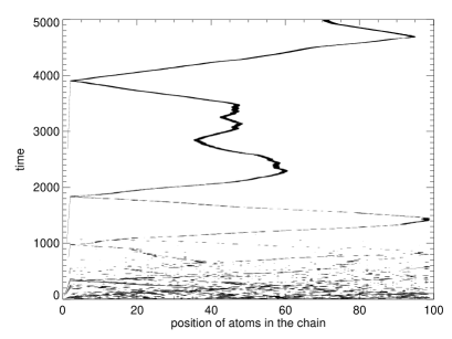
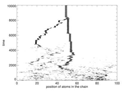


In Fig. 1 we show the space–time contour plots of the symmetrised site energies, defined as
The instantaneous total energy of the system is then given by . We see that a single localised excitation emerges from the relaxation process for both small and large values of . The pathway to localisation is the same as the one observed in the FPU model noi . In particular, the basic mechanism leading to localisation is modulational instability of short wavelength modes. The latter can only be effective if dissipation of long wavelength phonons is fast enough. As it shows from Eq. (2), this occurs only in the case of free–ends BC, whereas fixed–end BC strongly inhibit such process. On the other hand, breather mobility is strongly reduced in the highly discrete system (Fig. 1 (b)). Such difference is even more evident in the decay law of the normalized energy , which turns from pure exponential to stretched–exponential behaviour upon increasing . This is better appreciated by plotting the indicator
| (5) |
in a log–log scale, so that a stretched–exponential law of the form becomes a straight line with slope that intercepts the –axis at (Fig. 2 (a)). The scaling regions correspond to the onset of energy localisation, as can be seen by plotting the localisation parameter
| (6) |
(Fig. 2 (b)). From its very definition, the fewer sites the energy is localised onto, the closer is to . On the other hand, the more evenly the energy is spread among all the particles, the closer is to a constant of order 1. It should be noted, that is a relative quantity, and bears no information on the amount of energy that is localised. As a matter of fact, the fraction of that gets trapped in the residual state is found to be greater the higher the degree of discreteness of the system.
To summarise, if the on–site force is weak enough, the behavior is basically the same as the FPU chain which, in turn, exhibits in the approach to the residual state the same exponential decay law of its linearised counterpart, i.e. (see Eqs. (3)). The reasons for such behaviour are the same discussed for the FPU model noi . First of all, an effective harmonic Hamiltonian with energy–dependent renormalized frequencies is known to account for several equilibrium properties of the FPU chain Alabiso ; Lepri . Second, the harmonic approximation becomes increasingly accurate as time elapses, simply because more and more energy is extracted from the system by the reservoir. On the contrary, if the system is highly discrete, the first relaxation stage is indeed described by a stretched exponential law. A quantitative explanation of it is still lacking, but it is clear that in this case an effective description of such genuine non–linear phenomenon in terms of quasi–harmonic modes breaks down. In other words, the resulting interactions among linear modes inhibit the energy flow from the bulk to the boundaries, thus slowing down the dissipation.
The onset of a pseudo–stationary state corresponds in Fig. 2 to the almost flat final portions of the curves. Actually, being the system globally dissipative, energy is still at that stage exponentially decreasing but with a huge time constant . The latter is expected to be inversely proportional to the breather amplitude at the lattice edges, which, in turn, should be of order , with being the localisation length.
The above scenario is generic for large enough systems. Nonetheless, failure to spontaneously localise energy occurs the more frequently the smaller is the lattice. This is because the probability of occurrence of large enough energy fluctuations at a given energy density decreases with the number of particles. In other words, given a number of different initial equilibrium conditions, only a fraction of them will give rise to breathers. To give a quantitative idea, for the FPU model with , is only about 50 % for a chain of particles but rapidly approaches 100 % already for . In the absence of spontaneous localisation, the non–linear systems show no difference with respect to the linear ones and decays according to Eqs. (3).
II.3 The effective–exponent analysis
We have repeatedly mentioned that for the FPU model no stretched exponential relaxation is observed, even in presence of a weak on–site force. In this section we wish to remark this statement by reporting a more detailed analysis of the energy decay. This can be accomplished by defining an effective exponent through the logarithmic derivative
| (7) |
It is clear from definition (7) that if a portion of the energy decay curve goes as this would result in a plateau of height in the corresponding curve. For the problem at hand, interpretation of numerical data with this indicator is however a delicate matter. Actually, we want to remark that a naive analysis can lead to misleading or even incorrect conclusions reigada1 ; reigada2 .
The most convincing way to illustrate this is to discuss the case of the harmonic chain where localisation and stretched-exponential behaviour are obviously excluded a priori. From Eq. (3), it is easily seen that should start from 1 and monotonically vanish as for . On the other hand, we already learnt that in a finite chain a further crossover to an exponential law occurs so that must approach again 1 for . The net results of those competing trends is that, for a finite , displays a broad minimum , at . The value (which is independent of ) can be estimated by noting that from Eqs. (7) and (3) one has for , and hence . A simple plot of the curves shows how the the minimum can be incorrectly interpreted as a plateau if observed on a too short time scale. Of course, the same scenario is likely to appear in relatively short FPU chains whenever the chosen initial conditions do not yield localisation (see Fig. 3).


When localisation does occur, the residual state decays exponentially noi . Therefore one expects to converge to 1 as the residual state is approached. Actually, one observes first very small values of , while such a convergence does occur only on much longer time scales. To see why, let us consider a one–breather residual state. The total energy decays as , where is the initial energy of the breather and its characteristic decay time. The time constant is huge: in fact, it is roughly inversely proportional to the breather amplitude at the edge sites of the chain. From definitions (7) and (5) one has
| (8) |
Since is a number of order 1, we see that, at times such that , is very small. The numerical results in this case are just a deceptive byproduct of the wrong normalization. The exponent will start converging to 1 only when , which is a huge time, being also . In this case the analysis may be misleading in identifying the nature of the decay law. The way around such problem would be to calculate the effective exponent by normalizing the total energy to . However, this solution is in turn complicated by the intrinsic uncertainty in locating the time origin for the decay of the breather state.
III 2D lattices
Since a careful study of the 2D Klein-Gordon model has already been presented Aubry2 , we focus here on the 2D FPU model. In this respect, the most natural extension of model (II) should involve a two–component displacement vector. For the sake of simplicity, we rather consider here a scalar model with only one degree of freedom per lattice site. Actually, a preliminary series of simulations of the 2D vector version showed no appreciable differences with what reported here, and will be discussed elsewhere.
With the same choice of non–dimensional units introduced in section II, the model on a lattice () with damping on all edges is defined by the equations of motion
where , with . Since localisation has been shown to be strongly inhibited by fixed–ends boundary conditions, we consider here free–ends BC.
Calculations identical to the one described in section II.1 can be easily extended to the case of a simple 2D harmonic lattice. It turns out that the contributions from the two spatial coordinates are identical for an lattice, and therefore factorize, yielding
| (9) |
with . In particular, the law (9) applies in the absence of localisation, as well as during the first stage before the onset of localisation. In Fig. 4 we plot the energy decay curves of an FPU lattice with relaxing from different values of the energy density . The first stage of the decay indeed follows the theoretical prediction Eq. (9). Moreover, it is clear that localisation does not occur below a finite value of (located between and in this case). In particular, in the absence of localisation the energy decay is again described by the two–crossover scenario. Notice that, also in this case, failure to spontaneously localise energy results in a minimum of the effective exponent , due to the competition of the power law decay and the exponential law .


III.1 Fluctuation–activated localisation
The relaxation process described in terms of the energy decay curves is identical to the two–crossover picture which applies to the 1D FPU case. Nonetheless, the scenario markedly differs from the 1D case in two respects. First of all, the mobility of the localised excitations which spontaneously emerge is drastically reduced. In fact, after a first stage in which strong interaction is observed, they arrange on a “random lattice”, which, on the time scale of our typical simulations, appears indeed to be frozen. One of such states is illustrated in Fig. 5 (a). This is presumably due to a smaller “scattering section” in 2D. Obviously, due to the presence of dissipation, this state decays on a much longer time scale, which (as discussed above) scales exponentially with the linear size of the lattice.
The second important difference with the 1D case stems from the appearance of a finite energy threshold for the existence of breathers (akin to envelope solitons in the small–amplitude limit) in 2D 2D_tresh . As a consequence, we expect that localised modes are generated in the relaxation dynamics only by fluctuations that are large enough to overcome such threshold. The spontaneous excitation of breathers can thus be seen as an activated process. Accordingly, their number will be exponentially small in the ratio between and some quantity measuring the strength of fluctuations. Therefore, one expects the average density of breathers (i.e. the average number of breathers per lattice site) in the residual state to follow an Arrhenius law of the form
| (10) |
From Eq. (10), it is tempting to identify with some inverse temperature. However, one has to keep in mind that we are dealing with a non–equilibrium process and this identification can only make sense if energy release is adiabatically slow. If this is true, should be proportional to (and smaller than) the initial temperature, which, in turn, is roughly proportional to the initial energy density.
In our numerical simulations we clearly observe that strongly depends on the initial specific energy. In Fig. 5 (b) we plot for two system sizes as a function of , along with a fit performed with the law , with . As it shows, the agreement is good. We conclude that the spontaneous localisation of energy in our system is indeed an activated process. In particular, the fit gives . We note that a quantitative analysis of the time required to reach the residual state (localisation time) reveals that Esc_proc . By fitting the numerical data for the localisation time, it is possible to get an independent confirmation of the thermal activation scenario. In particular, we get , in good agreement with the value obtained above.
III.2 Statistics of breathers’ energies
It is important to realize that the “pseudo–stationary” distribution of breathers in the residual state emerges as a result of two competing mechanisms, namely the birth out of fluctuations from the homogeneous state and the decay due to both the coupling with the external reservoir and to the various inelastic interactions (phonon–breather, breather–breather etc). Although the former can be safely neglected, it is very difficult to understand the latter in full detail. Indeed, to the best of our knowledge, only a few studies are available Johansson ; Bang and a full description in terms of elementary interactions seems hardly feasible. Nonetheless, simple statistical arguments can be of help in understanding the energy distribution to a greater detail. Let us consider the fraction of breathers having energy between and with (in the FPU model breathers of arbitrarily large energy exist due to the unboundedness of the interaction potential) and let us define and to be some phenomenological birth and decay rates, respectively. Furthermore, let us assume that birth of a breather can only occur by a spontaneous fluctuation from the ground state (). Stationarity requires the flux–balance condition
| (11) |
Since the birth is an activated process we expect 111In principle, one could have a further energy–dependent prefactor in front of the exponential. That would affect the form of the distribution. We neglect it for simplicity. . This assumption yields (for a constant )
| (12) |
In this simplified description, the prefactor of the exponential term is thus interpreted as a measure of the effective breather lifetime () and is a priori unknown. In all simulations we observe that small–amplitude breathers decay more easily. This observation agrees with the accepted existence of a preferred energy flow from small–amplitude breathers to large–amplitude ones in breather–breather collisions Bang . Moreover, Eq. (12) requires that . Thus, we postulate
| (13) |
where the exponent can be estimated by measuring the distribution of breather energies in the vicinity of the threshold . We can estimate the average density of breathers in the residual state from Eqs. (12) and (13) as
| (14) |
This result is consistent with our initial hypothesis (Eq. (10)).
From Eqs. (12) and (13) it follows that the average breather energy can be expressed as a function of and . Hence, we can write the normalised distribution Eq. (12) as a function of the three parameters , and in the following fashion
| (15) |
where is the gamma function and . From the point of view of the numerics, it is more accurate to deal with the cumulative (integrated) distributions. These are easily obtained from the histograms without actually performing the integration, by noting that they are nothing but rank–size plots with the axes inverted. The cumulative distribution of the function (15) is
| (16) |
where is the incomplete gamma function, defined as
| (17) |
In principle one could evaluate explicitly by calculating the energy of exact breather solutions of vanishing amplitude 2D_tresh . However, we expect that . Therefore, if the population of breathers used to calculate the experimental distribution is large enough, we can assume that the smallest breather energy recorded is close to the threshold . Hence, we can perform a two–parameter fit with the theoretical prediction Eq. (16) with .
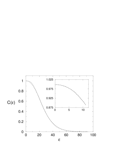
The quality of such fits is illustrated in Fig. 6 for a lattice with . As it shows, the agreement of our simple model with the numerics is excellent. In particular, the analysis of the small–energy portion of the distributions yields (see inset in Fig. 6). We stress that the result of our fits were well reproduced irrespective of the particular realisation of . The fit of the experimental distributions over the whole range of available energies yields a slightly greater value, . This is because the large–energy tail of the distributions accounts for the rarest events, which are under–represented within reasonably large breather populations 222The main constraint comes from the time required to numerically integrate the equations of motion of large lattices for a large number of realisations of a given initial condition.. In order to convince oneself that this is the case, it is enough to introduce an energy–dependent weight function in the fit, which gauges the relative weights of the small–energy and large–energy portions of the curves. In this case, the best estimates of monotonically decrease towards the value upon lowering the relative weight assigned to the large–energy region.

The analysis of energy distributions also provides an independent confirmation that localisation is in the present case an activated process. To check this, we fitted the distributions obtained by letting systems of given size relax from different values of . Then, we evaluated from the best–fit values of the fitting parameters and according to the relation
| (18) |
As shown in Fig. 7, turns out to be inversely proportional to as expected.
IV Conclusions
The mechanisms yielding the spontaneous formation of localised periodic excitations, i.e. breathers, in spatially discrete non–linear dynamical systems are of primary importance for the understanding of their physical interest. In this paper we have focused on the phenomenon of relaxation to breather states by cooling from the boundaries 1D and 2D lattices. We have provided a detailed description of the many facets of this phenomenon by combining numerical studies with theoretical arguments. In particular, we have shown that in models with sufficiently weak “substrate” forces the energy loss process can be explained on the basis of a simple perturbative analysis, that applies independently of the boundary conditions and of the nature of the nonlinearity. In this sense, we can claim that this is a general feature of this class of models, where an initial exponential decay is followed by a power–law behaviour. In the second stage of the decay process, boundary conditions play a crucial role in allowing for the formation of a long–living breather state, when they are taken free. On the contrary, fixed ends yield complete cooling of the lattice eventually ruled by the exponential decay rate of the longest–lived Fourier mode. We have also pointed out that the presence of a sufficiently strong “substrate” force can turn the initial exponential decay to a stretched–exponential law, while maintaining all the other features of the previously described scenario. A theoretical explanation of the origin of this stretched exponential behaviour and its dependence on the strength and on the nature of the local potential is a problem that deserves further and more refined investigations. We have also commented about the technical difficulties that can be encountered for identifying the correct time behaviour in these models, where the crossover between different regimes can be easily mistaken for an indication in favour of other scaling laws.
Another crucial aspect that we have widely analysed concerns the main differences between 1D and 2D systems. At variance with the former case, in 2D we have found numerical evidence of the existence of a finite energy threshold for breather formation. We have also proposed a statistical model that provides an effective agreement with numerical results concerning the breather residual state. This state eventually sets in as an almost static stationary configuration, where breathers of different amplitudes coexist. The statistical model is based on the hypothesis that this state emerges as a result of the competition between breather activation and mutual interaction. Moreover, it allows to determine an effective breather lifetime and its dependence on energy. In this framework the initial energy density plays the role of the control parameter regulating the strength of fluctuations.
In our opinion these results provide a satisfactory understanding of the phenomenon of spontaneous breather formation by cooling. As a final remark, it seems worth investigating experimentally the capability of real systems to store energy in the form of long–lived localised excitations.
Acknowledgements.
This work has been supported by the European Union under the RTN project LOCNET, Contract No. HPRN-CT-1999-00163. Francesco Piazza wishes to acknowledge numerous useful discussions with Katja Lindenberg.References
- (1) S. Flach and C. R. Willis, Phys. Rep., 295, 181 (1998).
- (2) S. Aubry and R. S. MacKay, nonlinearity 7, 1623 (1994).
- (3) T. Cretegny, T. Dauxois, S. Ruffo and A. Torcini, Physica D, 121, 109 (1998).
- (4) G. P. Tsironis and S. Aubry Phys. Rev. Lett. 77 (26) 5225 (1996).
- (5) A. Bikaki, N. K. Voulgarakis, S. Aubry and G. P. Tsironis, Phys. Rev. E 59 (1) 1234 (1999).
- (6) F. Piazza, S. Lepri and R. Livi, J. Phys. A, 34, 9803 (2001).
- (7) K. O. Rasmussen, A. R. Bishop and N. Gronbech–Jensen, Phys. Rev. E 58 R40 (1998).
- (8) I. Daumont, T. Dauxois, M. Peyrard, nonlinearity 10 617 (1997).
- (9) Yu. A. Kosevich and S. Lepri, Phys. Rev. B 61 6 (2000).
- (10) R. Reigada, A. Sarmiento and K. Lindenberg, Phys. Rev. E 64 066608 (2001).
- (11) R. Reigada, A. Sarmiento and K. Lindenberg, Physica A 305, 467 (2002).
- (12) C. Alabiso, M. Casartelli and P. Marenzoni, J. Stat. Phys, 79 451 (1995)
- (13) S. Lepri, Phys. Rev. E 58 (6) (1998).
- (14) S. Flach, K. Kladko and R. S. MacKay, Phys. Rev. Lett. 78 1207 (1997).
- (15) F. Piazza, S. Lepri and R. Livi, Localisation as an activated process in 2D non–linear lattices, World–Scientific (2002). In preparation.
- (16) M. Johansson and S. Aubry, Phys. Rev. E 61 5864 (2000).
- (17) O. Bang and M. Peyrard, Phys. Rev. E 53 4143 (1996).