Effects of Pore Walls and Randomness on Phase Transitions in Porous Media

I Introduction

Critical phenomena are generally well understood but the effects of randomness on the nature of the transitions are less well-studied. This is especially true in the case of phase transitions that take place in porous media where the effects of quenched randomness are provided by the pore walls. Among the best studied, are phase transitions in highly porous aerogels [1] — both the liquid - vapor transition [2] and the $\lambda$ - transition of ⁴He [1, 3, 4] have been found to be remarkably sharp. Even more interestingly, the topology of the phase diagram for ³He-⁴He mixtures in aerogels has been found to be different from that in the bulk [1, 5].

The simplest theoretical framework for studies of critical phenomena in non-random systems is the Ising model. The important role played by multiple length scales at a critical temperature $T_{c}$ leads to universality [6, 7, 8] — binary alloys which are about to order, binary liquids which are about to phase separate, certain kinds of magnets with uniaxial anisotropy which are about to become magnetized all exhibit the same critical behavior as the Ising model. Perhaps the simplest extension that incorporates randomness is the random field Ising model (RFIM) wherein a quenched random field is applied at each site [9, 10, 11]. One example of the probability distribution is the symmetric bimodal distribution which corresponds to a situation in which half of the sites experience an up field and the other half, a down field of equal strength. Another example involves fields which are Gaussian-distributed. In both cases, the symmetry between the up and down directions is not broken by hand and thus provides a scope for a spontaneous symmetry breaking and a phase transition associated with it.

Recent research [12, 13, 14, 15, 16] has lead to the result that the two probability distributions may correspond, at least in dimensions 3 and larger, to distinct behaviors associated with the RFIM. The Gaussian case is governed by a $T$=0 fixed point while the bimodal model’s phase diagram is qualitatively different. The origins of the two distinct scenarios relate to their quite different $T$=0 phase diagrams.

Experimental realizations of the RFIM include dilute antiferromagnets in a uniform field [17, 18, 19, 20] and binary liquid mixtures in a porous medium [21, 22, 23, 24, 25, 26, 27, 28]. In both these cases, many of the expected signatures associated with the RFIM with a Gaussian distribution of random fields were observed [17, 18, 19, 20] (but significant deviations were also found when the disorder was correlated [20]). However, the sluggish dynamics and irreversibility predicted by the theory [10, 11, 29] precluded accurate measurements of the exponents for binary liquids in porous media. Nevertheless, the exponents determined for the dilute Ising antiferromagnet in a uniform field were in accord with the theory.

A major surprise in this field were the measurements by Chan and his collaborators [2, 30] on the liquid-vapor transition of helium and hydrogen in a variety of porous media. While the liquid-vapor coexistence region was considerably shrunk compared to the bulk uniform case, the exponents were found to be much more akin to those of the uniform Ising model instead of the RFIM. It has been suggested [31, 32] that these features are related to the properties of the RFIM with the fields being distributed bimodally (though not necessarily symmetrically).

Another surprise was the novel shape of the experimentally determined [1, 5, 33] phase diagram of the ³He-⁴He mixtures in porous media which allowed for superfluidity at large concentrations of ³He. The classical aspects of this phase separation are captured by the Blume-Emery-Griffiths (BEG) [34] spin-1 model with an anisotropy. The presence of a porous medium can be modeled by making this anisotropy random with a bimodal distribution[35].

In this paper, we focus on the role played by pore walls in liquid-vapor transitions in porous media, as studied in their corresponding spin $\frac{1}{2}$ Ising spin systems. There are two aspects to the role of walls in a porous medium. First, there is a preference for one of the phases over the other in the vicinity of the walls. This mechanism alone ought to lead to observable consequences even when the placement of the walls is substantially periodic, i.e. the different phases are connected but there is no inherent randomness. Second, the random placement of the walls in the porous medium provides quenched disorder and can induce further changes in the phase behavior. The principal result of our paper is that the former aspect is more crucial – indeed, we show that within the framework of simple models, the phase diagram does not change on incorporating randomness. This finding is consistent with the analysis by Galam and Aharony [36] indicating that the mean field results of a ferromagnet in a random longitudinal field are the same as a uniaxially anistropic antiferromagnet in a uniform field. Our results suggest that liquid-vapor transitions in designed porous media, with a periodic geometrical pattern [37, 38], ought to exhibit behavior quite akin to that observed in random porous media. We demonstrate these findings in simple mean field Ising models and two distinct values of the local magnetic fields. We then generalize these studies to spin 1 Ising models with non-uniform anisotropy and show that such systems behave like the random anisotropy BEG systems with a bimodal distribution of the anisotropies [35]. Our results suggest that the ³He-⁴He phase separation is also primarily governed by the mere presence of walls in the porous medium and not randomness.

It should be noted that there have been several recent mean field studies of phase transitions in random porous media [39, 40, 41]. One would expect that fluctuations in lower dimensions [42] could play a key role in qualitatively modifying the mean field picture.

II Effects of Confinement Random in the Field Ising Model – the Symmetric Case

We start by considering the simplest case – that of four Ising spins located at two kinds of sites, 0 and 1, as shown in Figure 1a. Periodic boundary conditions are adopted in the plane of the figure. Furthermore, it is assumed that above and below this plane, there are spins which sit in locations that repeat the pattern shown and allow for a connected string of nearest neighbor 0 and 1 sites in the direction perpendicular to the plane of the paper. Physically, this geometry corresponds to a periodic arrangements of one-dimensional strings of 0 and 1 arranged on two sublattices. All spins are coupled by a uniform exchange constant, $J$. The magnetic field on sites 0 is denoted by $h_{0}$ and it points up. On sites 1, on the other hand, the magnetic field is equal to $h_{1}$ and it points down. (The case of a simple ferromagnet with a staggered field is obtained when periodic boundary conditions are adopted in all directions. One then does not have connected strings of 0 or 1 sites which lead to an inability to sustain certain phases at non-zero temperatures.)

Our objective here is to determine the phase diagram of this non-random system within the mean field approximation and compare it to the corresponding mean field results [31, 32, 43] of the RFIM in which the probability distribution of the magnetic fields is bimodal: half of the randomly selected sites have an up-pointing field $h_{0}$ and the other half – a down-pointing field $h_{1}$. The RFIM may be thought of as modeling porous media with the sites with field $h_{0}$ corresponding to locations near pore walls and the sites with field $h_{1}$ to the interior locations. The underlying assumption here is that there is a different environment near the pore wall than in the interior.

The phase diagram is obtained in the three-dimensional space of $h_{0}$, $h_{1}$, and $T$ and is determined by solving the following equations for the magnetizations $m_{0}$ and $m_{1}$:

$$m_{0}\;=\;tanh[(h_{0}+2Jm_{0}+4Jm_{1})/k_{B}T]\;\;,$$ (1)

$$m_{1}\;=\;tanh[(-h_{1}+4Jm_{0}+2Jm_{1})/k_{B}T]\;\;,$$ (2)

on sites with field $h_{0}$ and $h_{1}$ respectively. The solution is obtained in an iterative manner that leads to self-consistency. The form of equations (1) and (2) reflects the fact that each site of a given kind has four neighbors of the other kind and two neighbors of the same kind – the latter resulting from the out-of plane connectivity. Once the solutions for the local magnetizations are found, one can determine the free energy, $F=U-TS$, by calculating the internal energy

$$U\;=\;-2J(m_{0}m_{0}+m_{1}m_{1}+4m_{0}m_{1})-2h_{0}m_{0}+2h_{1}m_{1}$$ (3)

and the entropy

$$S=2s_{0}+2s_{1}\;\;,$$ (4)

where

$$s_{i}=-k_{B}\frac{1}{2}[(1+m_{i})ln(1+m_{i})/2+(1-m_{i})ln(1-m_{i})/2]\;\;.$$ (5)

A first order phase transition is identified by the presence of a cusp in the free energy.

It is easy to show that there are three possible phases at $T$=0 in this system. We shall denote them by +, $-$, and $+-$ and their energies by $E_{+}$, $E_{-}$, and $E_{+-}$ respectively. In the first phase, all spins are up and in the second all spins are down. In the third phase, on the other hand, the spins point in the directions of the local magnetic fields.

At $T$=0, the + and $-$ phases coexist along the diagonal direction in the $h_{0}-h_{1}$ plane (until $h_{0}=h_{1}=4J$), as shown in the top left panel of figure 2. The $+-$ phase coexists with the + phase along $h_{1}=4J$ for $h_{0}>4J$ and with the $-$ phase along $h_{0}=4J$ for $h_{1}>4J$. All of the phase boundaries at $T$=0 are first order lines denoted by dashed lines. The solid lines denote lines of continuous transitions. Two of these lines occur close to $T=2J/k_{B}$ and separate the $+-$ phase from the $+$ and $-$ phases respectively. The star in the main phase diagram, where three critical lines come together, is a tricritical point. The critical line corresponding to the transition between + and $-$ starts at 6$J/k_{B}$ when $h_{0}$ and $h_{1}$ tend to zero and then decreases steadily as the fields are increased. In the vicinity of $h_{0}=h_{1}$=$\;4J$, the descent towards the tricritical point is almost vertical.

A particularly simple case is obtained on fixing $h_{0}$ at the value of $6J$ (corresponding to strong pinning at the pore wall) and varying $h_{1}$ and $T$ to map out the coexistence curve between the + and $+-$ phases. In order to cancel the effective field introduced by the nearly fully aligned $m_{0}$ spins, one needs to impose a field $h_{1}=4J$ (note that each site ’1’ has four ’0’ neighbors) and effectively one is left with the bulk Ising model. Figure 3 shows that the coexistence manifests itself in the presence of two values of $m_{1}$ but a unique value of $m_{0}$. Of course, a similar scenario takes place when the boundary between $-$ and $+-$ is crossed. What is quite remarkable is that the topology of the phase diagram does not change even when randomness is introduced [31, 32, 43] in such a way that the symmetry between the + and $-$ phases is maintained. Thus within mean field theory, for the symmetric case, the random placement of the walls plays no role at all. We will show in the rest of the paper that the same result holds for more complex situations.

III Effects of Confinement in the Random Field Ising Model – the Asymmetric Case

In porous media, the volume of a fluid near the pore walls is usually much less than the volume of the fluid in the interior. In the Ising spin model, this translates into an unequal number of sites with fields $h_{0}$ and $h_{1}$. In fact, in a random version of the model, we [31] considered a situation in which a fraction $p$ of the sites has a field $h_{0}$ – the symmetric case is obtained when $p=\frac{1}{2}$.

In order to study the effects of walls under such asymmetric conditions, we consider, for simplicity, the model shown in figure 1b which is a generalization of figure 1a. The plane of the figure shows nine sites. The central site, denoted by 0, has a local field of $h_{0}$. The remaining eight sites have a field of $h_{1}$ and they are denoted by 1 and 2. Thus $p=\frac{1}{9}$ but there is no randomness. The distinction between the two classes of sites, 1 and 2, is that the former have site 0 as a neighbor and the latter do not. Again, it is assumed that above and below the plane shown there are other planes which repeat the pattern of the central plane so that each site has a coordination number of six. Recall that the boundary conditions along the two directions within the plane are periodic.

The mean field equations for the three magnetizations read

$$m_{0}\;=\;tanh[(h_{0}+2Jm_{0}+4Jm_{1})/k_{B}T]\;\;,$$ (6)

$$m_{1}\;=\;tanh[(-h_{1}+Jm_{0}+3Jm_{1}+2Jm_{2})/k_{B}T]\;\;,$$ (7)

$$m_{2}\;=\;tanh[(-h_{1}+2Jm_{1}+4Jm_{2})/k_{B}T]\;\;.$$ (8)

The internal energy of the system is given by

$$U\;=\;-J(m_{0}m_{0}+6m_{1}m_{1}+8m_{2}m_{2}+4m_{0}m_{1}+8m_{1}m_{2})-h_{0}m_{0}+4h_{1}m_{1}+4h_{1}m_{2}$$ (9)

and the entropy by

$$S=s_{0}+4s_{1}+4s_{2}\;\;.$$ (10)

This system continues to have three phases at $T$=0 as indicated in the top left panel of figure 4. The boundaries between the phases, however, are shifted to new locations. For instance, the + and $-$ phases coexist along the line $h_{0}=8h_{1}$, from the origin until $h_{0}=4J$ The + and $+-$ phases coexist along $h_{1}=\frac{1}{2}J$ for $h_{0}>4J$ whereas the $-$ and $+-$ phases coexist along $h_{0}=4J$ for $h_{1}>J/2$. The triple point at which all the three phases coexist is at $T=0$, $h_{0}=4J$ and $h_{1}$=$\frac{1}{2}J$.

The emergence of the three phases is the only similarity that exists between the symmetric and the asymmetric model. The way they coexist at non-zero temperatures, for instance, is quite different. The biggest distinction, shown in the main panel of figure 4, is that now the two sheets separating the + phase from the $+-$ and the $+$ and $-$ phases along the diagonal direction combine together to form one surface. This surface has a tilt that is clearly visible on the right top panel of figure 4 which shows a section of the phase diagram at $k_{B}T=5.5J$. The surface terminates at a critical line which falls very gently from $k_{B}T=6J$ at $h_{0}=0$ and $h_{1}$=0 to about $5.5J$ at $h_{0}=8.5J$ and $h_{1}=0.42J$.

The coexistence surface of the $-$ and $+-$ phases continues to be substantially planar with a critical line close to 2$J$ reflecting the one-dimensional connectivity of the 0 sites. This line of critical points intersects the combined $+,-$ and $+,+-$ coexistence surface at a critical end point at $k_{B}T=2.05J$, $h_{0}=3.9612J$, and $h_{1}$=$\frac{1}{2}J$. Quite remarkably, the topology of this phase diagram is exactly as in the random case [31].

The coexistence curves for $h_{0}$=$6J$ (again mimicking a strong pore-wall interaction) are shown in Figure 5. Physically, the transition corresponds to crossing from a phase in which the interior of the pore space is filled by liquid to one in which the liquid coats the walls and the vapor occupies the interior. Note the unusual geometry of the coexistence curve. The magnetizations $m_{1}$ and $m_{2}$ have broad coexistence curves, similar to $m_{1}$ of Figure 3 for the symmetric case. On the other hand, the coexistence curve for $m_{0}$ is much narrower than for $m_{1}$ and $m_{2}$ and its non-zero width arises when the values of $m_{1}$ and $m_{2}$ are distinct. When $m_{2}=m_{1}$, $m_{0}$ has a unique value in analogy to the symmetric case. It should be noted that there are just two coexisting solutions – the larger value of $m_{0}$ selects positive values of $m_{1}$ and $m_{2}$, whereas the smaller values correspond to negative $m_{1}$ and $m_{2}$.

IV Novel Superfluid Phases in ³He–⁴He Mixtures in Aerogel

We turn now to a discussion of spin systems modeling the phase separation of ³He–⁴He mixtures. Figure 6(a) shows a sketch of the experimental phase diagram (in the temperature ($T$) - concentration of ³He ($x$) plane) of bulk ³He-⁴He mixtures in the vicinity of the superfluid transition of ⁴He. In the temperature range of interest, the superfluid transition involving the pairing of ³He atoms is not a factor and indeed the ³He atoms can be thought of as inert, annealed (i.e. they are not stuck in space but can move around) entities. At low ³He concentrations, on cooling the system, a superfluid transition denoted by the solid line (AB) is observed. However at higher ³He concentrations, the system opts to phase separate into a ⁴He rich region which becomes superfluid. The coexistence curve of the ³He-⁴He phase separation is shown as a dashed curve (CBD). Two interesting features of the phase diagram are the tricritical point B, where the superfluid transition line collides with the coexistence curve at its critical point and the miscibility gap at C – small amounts of ³He added to ⁴He do not lead to phase separation: a feature exploited in dilution refrigerators.

Perhaps, the simplest classical model that captures the topology of this phase diagram is the Blume-Emery-Griffiths model [34] (BEG) which is a lattice model populated with spins, $S_{i}$, that can take on one of three values 0, -1, or 1. The inert ³He is represented by 0 spins and ⁴He is denoted by +1 or 1 spin values. An exchange coupling between nearest neighbor non-zero spins, favoring alignment causes the analog of the superfluidity transition, with the broken symmetry phase having a non-zero magnetization (i.e. a mismatch in the number of +1 and 1 spins). The Hamiltonian reads

$$H\;=\;-J\sum_{<ij>}S_{i}S_{j}\;+\;\sum_{i}\Delta S_{i}^{2}\;\;,$$ (11)

where $\Delta$ is an anisotropy field which controls the relative concentrations of the two isotopes. The presence of ⁴He corresponds to $S_{i}=\pm 1$, superfluidity of ${}^{4}He$ to the existence of non-zero magnetization and the ³He atoms are represented by $S_{i}=0$. The random anisotropy field here does not break the $\pm$ symmetry.

The resulting phase diagram (shown in Figure 6b) has all the correct qualitative features, except for the absence of the miscibility gap at C which is believed to arise from a purely quantum mechanical effect. Even thought the BEG model is purely classical and does not have the correct symmetry of the spins (the superfluid transition has the same characteristics of the transition in a $xy$ model in which spins lie in a plane rather than having up-down symmetry), it nevertheless reproduces almost all the qualitative features of the experiment correctly.

Recent experiments of Chan and coworkers [1, 5, 33] on the phase separation of ³He-⁴He mixtures in aerogel in the vicinity of the superfluid transition have yielded a phase diagram shown Figure 6(c). The key features of the phase diagram are i) the absence of the tricritical point (the superfluid transition line no longer intersects the coexistence curve); ii) an enhancement of the superfluid transition temperature compared to the bulk at large ³He concentration iii) at low temperatures (below the critical point associated with the phase separation) and for a range of values of $x$ within the coexistence curve, ⁴He rich and ³He rich regions coexist, both of which are superfluid and iv) the experimental data, while restricted to temperatures above 0.35 K, are suggestive that the aerogel causes a miscibility gap to open up at large value of $x$. This is of fundamental importance, if true, since the superfluid phase observed is one in which a small quantity of ⁴He in ³He does not phase separate (as observed in the bulk), but is yet superfluid and probably represents the long sought after dilute Bose gas superfluid phase. Even more exciting, such a miscibility gap would lead to the extremely novel situation of two distinct coexisting superfluid phases at low temperatures, the dilute Bose gas phase of ⁴He and the superfluid phase of ³He. Two factors in support of the novel dilute superfluid phase are: a) Adding a small amount of ⁴He to the aerogel (in the absence of ³He) leads to a superfluid phase whose density is enhanced by the addition of ³He. b) Because a coexistence curve for the phase separation is found in the phase diagram, it is plausible that there is no phase separation in the region between B and D (6(c)), since it is unlikely to expect phase separation of an already phase separated phase.

V The Random Anisotropy BEG Model

In the BEG model the effect of the aerogel is assumed to be present on a fraction p of the sites, these sites are randomly chosen and fixed (unlike the mobile ³He atoms, the aerogel is a manifestation of quenched randomness). The distribution of the single site anisotropies is bimodal and given by [35]

$$P(\Delta_{i})=\;=\;p\delta(\Delta_{i}-\Delta_{0})\;+\;(1-p)\delta(\Delta_{i}-\Delta_{1})\;\;.$$ (12)

The sites with anisotropy $\Delta_{0}$ correspond to vicinity of pore walls and for the situation in which ⁴He prefers to be near the wall, $\Delta_{0}<0$. The $\Delta_{1}$ anisotropy characterizes the pore interior and its value controls the total number of ³He atoms. In a mean field approach, one obtains the phase diagram shown in Figure 6(d). Note that this is in accord with the experimental observations (i) and (iii), but does not reproduce (ii) and (iv). The tricritical point (where three phases go critical simultaneously) requires a special symmetry, which is absent when one incorporates the random anisotropy to mimic the aerogel. The line of superfluid transitions is, however, virtually insensitive to the presence of the random anisotropy. The coexistence curve, however, is shifted to lower temperatures and higher effective ⁴He concentration due to the space taken up by the aerogel, thus leading to the topology shown in Figure (6(d)).

In order to investigate whether this lack of complete agreement arises due to quantum mechanical effects and their neglect by the BEG model or due to the inherent simplicity of the mean field approach, we have carefully studied the BEG model within an improved mean field theory which is a generalization of the approach presented in Ref. [44]. The improved method captures features such as a percolation threshold and yield better estimates of the transition temperature than the mean field theory.

The phase diagrams 6(e) and (f) are obtained depending on whether the fraction $p$ of the sites at which the aerogel is present is less than or greater than the percolation threshold $p_{c}$. Unlike the porous medium aerogel, which has a strongly correlated, connected interface, our model, in its simplest form, consists of randomly chosen interface sites allowing for a percolation threshold. In the experiment, in spite of the large porosity, one is always in the fully connected regime. Note the presence of a miscibility gap at high ³He concentrations. Unlike mean field theory (6(d)), the point D is at a concentration less than $(1-p)$. Indeed, our calculations suggest a second coexistence curve between D and the point ($x=1-p$; $T$=0) analogous to the one between C and D except that the critical temperature is shifted down to zero. Thus for concentrations of ³He corresponding to points between D and ($x=1-p$; $T$=0), and temperatures less than the superfluid transition line AB, the model predicts the analog of the dilute Bose gas superfluid phase.

The superfluid transition temperature smoothly extrapolates to the value of the transition temperature of a coated phase of helium atoms residing on the aerogel surface. This is dramatically seen in Figure 6(f) where the transition plunges to zero at $x=1-p$ when $p$ is less than the percolation threshold $p_{c}$ and is unable to sustain a phase transition at non-zero temperatures. Within the context of the BEG model, the novel superfluid phase is found to be one in which the magnetization (superfluidity) arises from the aerogel sites and from the sites in their vicinity. Indeed, in any classical model with short range interactions, the spins yielding a non-zero magnetization must lie on a connected cluster and are thus in an essentially phase separated phase. This phase separation, however, does not preclude a further bulk-like phase separation on increasing the concentration of ⁴He atoms. In our BEG model, the minimum number of ⁴He atoms is equal to the number of aerogel surface sites. A further addition of ⁴He atoms (in the absence of ³He) causes an increase in the magnetization, corresponding to the attachment of some of these atoms to the already existing spanning cluster at the aerogel surface. Subsequent addition of ³He atoms results in more of the ⁴He atoms going in the cluster, thereby enhancing the magnetization, as in the experiment. We have also studied the effects of correlation in the selection of aerogel surface sites: the probability of a nearest neighbor site of an aerogel surface site to be another aerogel surface site is enhanced compared to a completely random selection. We find this correlation enhances the superfluid transition temperature compared to the bulk in accord with experiment.

In summary, a simplified model for ³He-⁴He mixtures in aerogel reproduces many (but the miscibility gap at low ³He concentrations) of the features observed in experiments and suggests the opening of a miscibility gap at low ⁴He concentration. The analog of the dilute Bose gas phase within the classical model is one in which the superfluidity arises from ⁴He adsorbed on the aerogel. Note that this does not however preclude further phase separation. Cooling the system to ultralow temperatures in the miscibility gap at high ³He concentrations should lead to two coexisting superfluid phases: ³He and the ⁴He near the aerogel. It would be very exciting if quantum mechanical effects (not considered here) delocalize the ⁴He atoms leading to a dilute Bose gas phase at higher temperatures and interpenetrating ⁴He and ³He superfluid phases at low temperatures.

It should be noted that much of the physics corresponding to the scenarios of Figure 6 has been captured by the renormalization group analysis of Berker and his collaborators [45, 46, 47, 48]. They considered random and non-random ”jungle-gym” models of the aerogel and explained the phase diagrams by the connectivity and tenuousness of the aerogel.

VI Effects of Confinement in the BEG model

In order to study the separate roles of the presence of walls and randomness on ³He–⁴He separation, we again consider the geometry shown in Figure 1b and set up mean field equations that correspond to the spin-1 problem. These equations for the magnetizations, i.e. the expectation values of $S_{i}$, and for the three parameters $q_{0}$, $q_{1}$, and $q_{2}$ which are the expectation values of $S_{i}^{2}$, are:

$$m_{0}\;=\;q_{0}\;tanh[(2Jm_{0}+4Jm_{1})/k_{B}T]\;\;,$$ (13)

$$m_{1}\;=\;q_{1}\;tanh[(Jm_{0}+3Jm_{1}+2Jm_{2})/k_{B}T]\;\;,$$ (14)

$$m_{2}\;=\;q_{2}\;tanh[(2Jm_{1}+4Jm_{2})/k_{B}T]\;\;,$$ (15)

and

$$q_{i}\;=\;\frac{4\;\exp{(-2\Delta_{i}/k_{B}T)}-\sqrt{m_{i}^{2}+4\;\exp{(-2\Delta_{i}/k_{B}T)}\;(1-m_{i}^{2})}}{4\;\exp{(-2\Delta_{i}/k_{B}T)}-1}\;\;.$$ (16)

The internal energy is given by

$$U\;=\;-J(m_{0}m_{0}+6m_{1}m_{1}+8m_{2}m_{2}+4m_{0}m_{1}+8m_{1}m_{2})+\Delta_{0}q_{0}+4\Delta_{1}q_{1}+4\Delta_{1}q_{2}$$ (17)

and the entropy by

$$S=\tilde{s}_{0}+4\tilde{s}_{1}+4\tilde{s}_{2}\;\;,$$ (18)

where

$$\tilde{s}_{i}=-k_{B}[(1-q_{i})ln(1-q_{i})+\frac{1}{2}(q_{i}+m_{i})ln(q_{i}+m_{i})/2+(q_{i}-m_{i})ln(q_{i}-m_{i})/2]\;\;.$$ (19)

In direct analogy to the random case [35], there are four posssible phases at $T$=0:

  

phase 1 in which all three $m_{i}$s are non-zero;

  

phase 2 in which $m_{0}>0$, $m_{1}=m_{2}=0$;

  

phase 3 in which $m_{0}=0$, $m_{1}$, $m_{2}>0$; and

  

phase 4 in which $m_{0}=m_{1}=m_{2}=0$.

In each phase, $q_{i}$=$m_{i}$ at $T$=0. The non-zero magnetization persists to higher temperatures and its disappearance corresponds to the $\lambda$ line for superfluid ⁴He. (Note that our analysis lumps in any inert or dead layer of ⁴He as belonging to the pore wall.) The analog of the ³He concentration is given by

$$x\;=\;1\;-\;(q_{0}+4q_{1}+4q_{2})/9\;\;.$$ (20)

The overall topology of the phase diagram is shown on figure 7 and several isothermal slices through it are shown in figure 8. At low temperatures all four phases exist and their number goes down on increasing the temperature. The $T$=0 boundaries are given by

  

1 – 2 coexistence at $\Delta_{1}=\frac{13}{4}J$, $\;\Delta_{0}<J$;

  

1 – 3 coexistence at $\Delta_{0}=5J$, $\;\Delta_{1}<\frac{11}{4}J$;

  

1 – 4 coexistence $\Delta_{1}=\frac{27}{8}J-\frac{1}{8}\Delta_{0}$, $\;J<\Delta_{0}<5J$ ;

  

2 – 4 coexistence at $\Delta_{0}=J$, $\;\Delta_{1}>\frac{13}{4}J$;

  

3 – 4 coexistence at $\Delta_{1}=\frac{11}{4}J$, $\;\Delta_{0}>5J$.

These first-order boundaries become vertical surfaces on considering the $T$-axis. The top edges of these surfaces are critical lines. This has as its roof a critical surface at which the magnetization disappears. Of course phase 4, which is paramagnetic, is not covered by a roof. This roof corresponds to the superfluid transition of ⁴He or the $\lambda$ - line. The shape pf the roof is illustrated in figure 9 for several values of $\Delta_{0}$. In the figure, for $\Delta_{0}/J\leq 0.8$, the roof continues indefinitely for large $\Delta_{1}$, becaouse $m_{0}$ remians zero at sufficiently low temperatures. However, when $\Delta_{0}/J$, the roof smoothly terminates at the top of the wall separating planes 1 and 4. This is necessitated by the fact that phase 4 has no roof.

Figure 10 illustrates the nature of the phase diagram for selected values of $\Delta_{0}$. The insets show the transition lines as a function of $\Delta_{1}$ and the main figures – as a function of $x$ – the analog of the ³He concentration. The top two panels of Figure 10 refer to the uniform anisotropy case - when $\Delta_{0}$ is equal to $\Delta_{1}$ and confirm that this simple nine-spin model captures the topology of the phase diagram of the uniform BEG model [34].

The physically interesting regime is that of negative $\Delta_{0}$ which favors ⁴He near the pore walls. It is seen that, as $\Delta_{1}$ is varied, the $\lambda$ line becomes disconnected from the phase separation coexistence lines (the middle panels). The details depend on how one moves on the $\Delta_{0}$ - $\Delta_{1}$ plane. For instance, if one crosses the 1–2 and 2–4 boundaries at an angle, one gets the situation depicted in the bottom panels of Figure 10. All of these phase diagrams are in accord with the random anisotropy version of the model except that the $\lambda$ line of the bottom panels of figure 10 does not reemerge from the ³He-⁴He coexistence region because, this region ends at $x$=1 in this simple model, and not at an $x$ which is less than 1. Figure 11 shows the coexistence curves for the $q$ order parameters for $\Delta_{0}$=-0.5$J$. They are remarkably similar to the magnetization coexistence curves of Figure 6. In particular, the non-zero width for the coexistence region in $q_{0}$ reflects inequality of $q_{1}$ and $q_{2}$.

The basic message of our analysis is that the topology of the phase diagram changes qualitatively (in accord with experiment) when one moves in the $(\Delta_{0}-\Delta_{1})$ plane such that instead of going directly from phase 1 to the paramagnetic phase 4, one moves through the intermediate phase 2. Somewhat surprisingly and at odds with expectations, one finds that the mean field topology of the phase diagram is more sensitive to the presence of walls in a porous medium than to the role played by their random placement. A similar conclusion has been reached by Pricaupenko and Treiner [49] within a nonlocal density functional analysis of ³He-⁴He mixtures in a channel geometry. In particular their analysis shows possibility of the detachment of the superfluid line from the coexistence region. It would be interesting to consider whether fluctuations make a qualitative difference in the conclusions reached in our simple mean field analysis.

We are indebted to Moses Chan for stimulating discussions. This work was supported by the Center of Collective Phenomena in Restricted Geometries, the Penn State MRSEC under NSF grant DMR-0080019, INFM, MURST, and NASA.

FIGURE CAPTIONS

  

Figure 1. a) The basic unit of the model used to study the symmetric case in which there are as many sites with the local field $h_{0}$, denoted by 0, as with the field $h_{1}$, denoted by 1. The 0s and 1s are placed on two sublattices in the plane as shown and is periodically repeated in both directions in the plane of the paper. The model has lines of 0 and 1 sites respectively perpendicular to the plane of the paper. In other words, the pattern shown is repeated in other parallel planes. b) The geometry of the model used to study the asymmetric case. The site denoted by 0 has a field $h_{0}$ and the remaining sites a field $h_{1}$. As before, there are periodic boundary conditioons in the plane and repeat boundary conditions in the direction perpendicular to the page.

  

Figure 2. The main panel shows the phase diagram corresponding to the symmetric case in a three dimensional representation $h_{0}-h_{1}-T$. The dashed lines correspond to first order transitions whereas the thick solid lines correspond to the continuous transitions. The star indicates a tricritical point. The top panels show constant temperature slices of the phase diagram for the temperatures indicated. The asterisk on the right hand panel indicates a critical point and the square on the top left panel is a triple point.

  

Figure 3. The temperature dependence of the local magnetizations, $m_{0}$ and $m_{1}$ on crossing the boundary between the + and $+-$ phases at $h_{0}=6J$. For temperatures below $T=2J$, there is a coexistence of two values of $m_{1}$ but $m_{0}$ stays essentially fully magnetized up to $T\;=\;2J$.

  

Figure 4. The main panel shows the phase diagram corresponding to the asymmetric case in a three dimensional representation $h_{0}-h_{1}-T$. The dashed lines correspond to first order transitions whereas the thick solid lines correspond to continuous transitions. The pentagon indicates a critical end point. The top panels show constant temperature slices of the phase diagram for the temperatures indicated. The asterisk on the right hand panel indicates a critical point, whereas the square on the top left hand panel is a triple point.

  

Figure 5. The temperature dependence of the local magnetizations, $m_{0}$, $m_{1}$, and $m_{2}$ on crossing the boundary between the + and $+-$ phases at $h_{0}=6J$. The coexistence curve for $m_{0}$ is much narrower than for $m_{1}$ and $m_{2}$. There are two coexisting solutions and the larger value of $m_{0}$ selects positive values of $m_{1}$ and $m_{2}$, whereas the smaller values correspond to negative $m_{1}$ and $m_{2}$.

  

Figure 6. Schematic representations of the experimentally (panels a and c) and theoretically determined phase diagrams for ³He-⁴He separation as described in more detail in the text. The phase diagram is shown in the temperature ($T$) – concentration of ³He ($x$) plane. Panels a) and b) correspond to experimental and theoretical results for the bulk case. All other panels refer to random situations. Panel c) corresponds to the experiments in aerogels. Panel d) corresponds to the mean field analysis of the random anisotropy BEG model with a bimodal distribution of the anisotropies. Panels e) and f) correspond to theoretical results in which $p$, the fraction of randomly chosen sites corresponding to the pore walls, is smaller or larger than the percolation threshold respectively.

  

Figure 7. The phase diagram for the BEG model with a bimodal non-random distribution of the anisotropies in a three-dimensional representation $\Delta_{0}-\Delta_{1}-T$. The broken lines correspond to the first order transitions whereas the solid lines correspond to continuous transitions.

  

Figure 8. Constant temperature slices of the phase diagram shown in Figure 7 at the temperatures indicated.

  

Figure 9. Plot of the critical lines (the temperature at which the magnetization goes to zero) as a function of $\Delta_{1}$ for the indicated values of $\Delta_{0}$.

  

Figure 10. Top left panel: The phase diagram for the uniform (bulk) anisotropy BEG model in the $T-x$ plane, where $x$ is the spin analog of the concentration of He³. Top right panel: The same phase diagram but in the $T-\Delta_{1}$ plane. $\lambda$ indicates the critical line for the magnetization and I the first order transition in the $q$-order parameter. Middle left panel: The phase diagram for the non-uniform (periodic) anisotropy BEG model in the $T-x$ plane. The data are for $\Delta_{0}\;=\;-0.5J$. Middle right panel: The corresponding phase diagram in the $T-\Delta_{1}$ plane. The bottom panels: The phase diagrams for for $\Delta_{0}=\Delta_{1}/5$.

  

Figure 11. The coexistence curves for the order parameter $q$ on the three sites when $\Delta_{0}=-0.5J$. There are two coexisting solutions and the larger value of $q_{0}$ selects larger values of $q_{1}$ and $q_{2}$.

FIG. 1.:

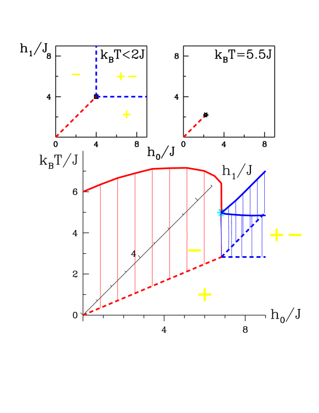
FIG. 2.:

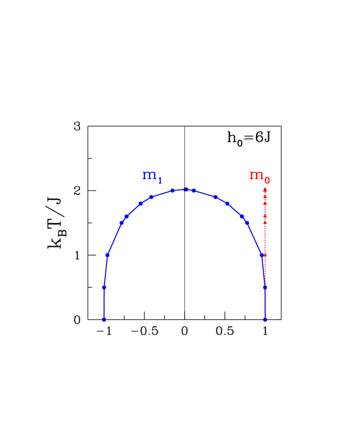
FIG. 3.:

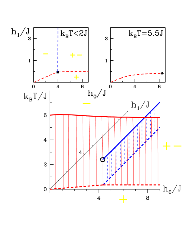
FIG. 4.:

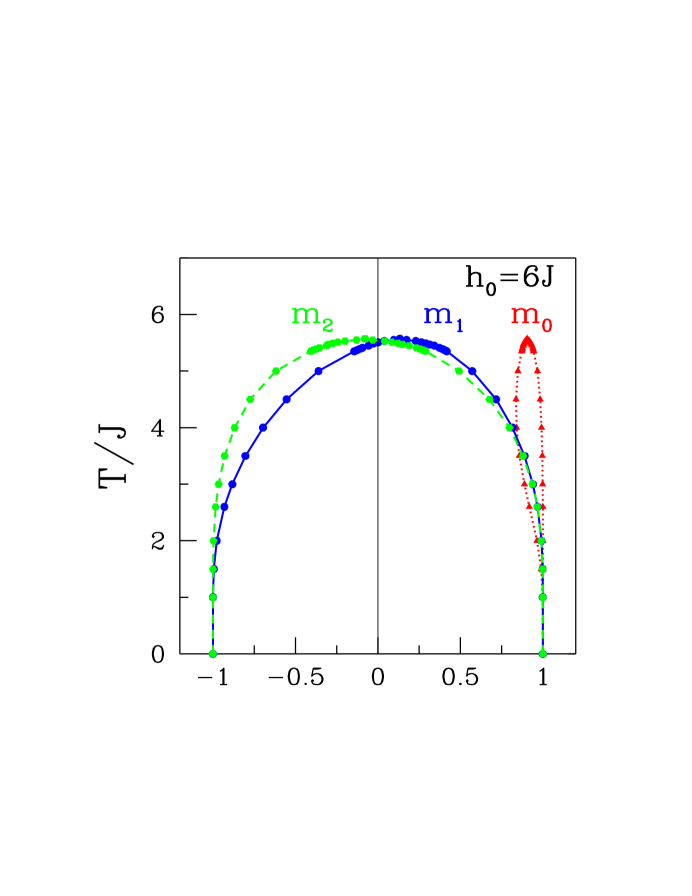
FIG. 5.:

FIG. 6.:

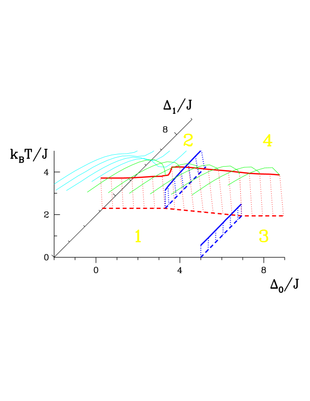
FIG. 7.:

FIG. 8.:

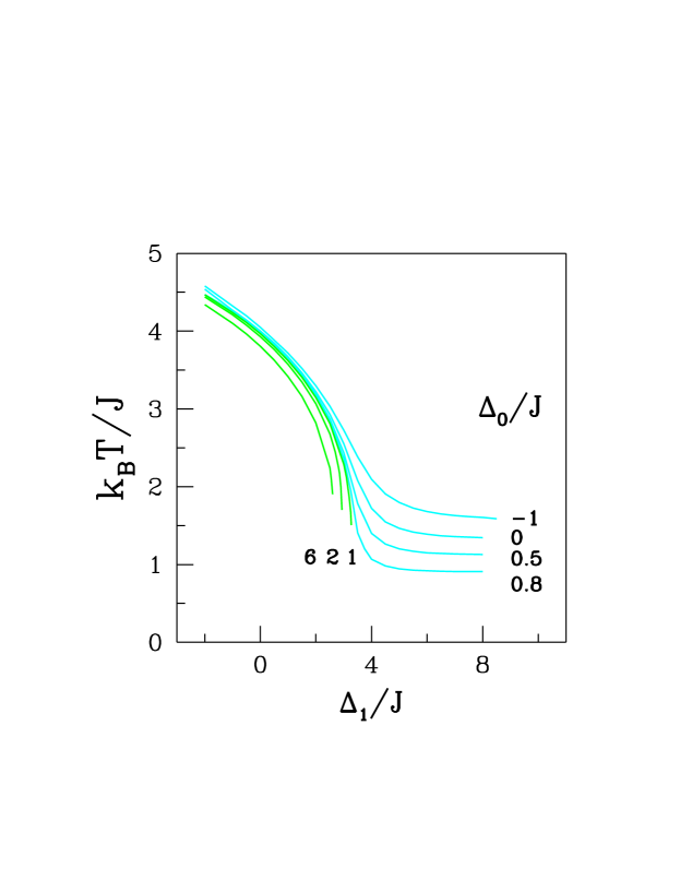
FIG. 9.:

FIG. 10.:

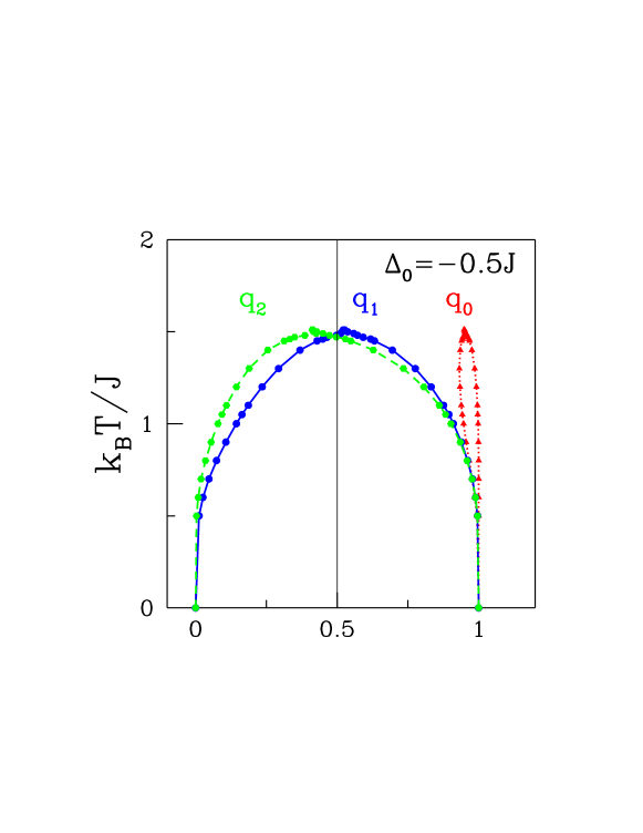
FIG. 11.:

REFERENCES

- [1] M. H. W. Chan, N. Mulders, and J. Reppy, Physics Today, 30–37 (August,1996).
- [2] A. P. Y. Wong, M. H. W. Chan, Phys. Rev. Lett. 65, 2567–2570 (1990).
- [3] M. H. W. Chan, K. I. Blum, S. Q. Murphy, G. K.-S. Wong, and J. D. Reppy, Phys. Rev. Lett. 61, 1950-1953 (1988).
- [4] G. K.-S. Wong, P. A. Crowell, H. A. Cho, and J. D. Reppy, Phys. Rev. B 48, 3858-3880 (1993).
- [5] S. B. Kim, J. Ma, M. H. W. Chan, Phys. Rev. Lett. 71, 2268-2271 (1993).
- [6] L. P. Kadanoff, Proc. of the Int. School of Phys. “Enrico Fermi” (Varenna) Course LI, Green, M. S., editor, Acad. Press, New York, 1971.
- [7] K. G. Wilson, Rev. Mod. Phys. 47, 773–840 (1975).
- [8] H. E. Stanley,Rev. Mod. Phys. 71, S358-S366 (1999).
- [9] Y. Imry, S. -k. Ma, Phys. Rev. Lett. 35, 1399–1401 (1975).
- [10] D. S. Fisher, G. M. Grinstein, and A. Khurana, Physics Today 41, Dec. 56–67 (1988).
- [11] D. P. Belanger and A. P. Young, J. Magn. Magn. Mater 100, 272–291 (1991).
- [12] M. R. Swift, A. J. Bray, A. Maritan, M. Cieplak, and J. R. Banavar, Europhys. Lett. 38 273–278 (1997).
- [13] J. -C. Angles d’Auriac and N. Sourlas, Europhys. Lett. 39, 473–478 (1997).
- [14] J. Esser, U. Nowak, and K. D. Usadel, Phys. Rev. B 55, 5866–5872 (1997).
- [15] A. K. Hartmann and U. Nowak, Eur. Phys. J. B 7, 105–109 (1999).
- [16] P. M. Duxbury and J. H. Meinke, cond-mat 0012042.
- [17] R. J. Birgeneau, R. A. Cowley, G. Shirane, and H. Yoshizawa, J. Stat. Phys. 34, 817-848 (1984).
- [18] P. Z. Wong, J. W. Cable, and P. Dimon, J. Appl. Phys. 55, 2377-2382 (1984).
- [19] D. P. Belanger, A. R. King, and V. Jaccarino, J. Appl. Phys. 55, 2383-2388 (1984).
- [20] J. P. Hill, Q. Feng, R. J. Birgeneau, T. R. Thurston, Z. Phys. B 92, 285–305 (1993).
- [21] J. V. Maher, W. I. Goldburg, D. W. Pohl, and M. Lanz, Phys. Rev. Lett. 53 60–63 (1984).
- [22] M. C. Goh, W. I. Goldburg, C. M. Knobler, Phys. Rev. Lett. 58, 1008–1011 (1987).
- [23] S. B. Dierker, P. Wiltzius, P. Phys. Rev. Lett. 58, 1865–1868 (1987).
- [24] P. Wiltzius, S. B. Dierker, and B. S. Dennis, Phys. Rev. Lett. 62, 804–807 ((1989).
- [25] S. B. Dierker, and P. Wiltzius, Phys. Rev. Lett 66, 1185–1188 (1991).
- [26] B. J. Frisken, F. Ferri, and D. S. Cannell, Phys. Rev. Lett. 66, 2754–2757 (1991).
- [27] F. Aliev, W. I. Goldburg, and X-l. Wu, Phys. Rev. E 47, R3834–3837 (1993).
- [28] M. Y. Lin, S. K. Sinha, J. M. Drake, X-l. Wu, P. Thiyagarajan, and H. B. Stanley, Phys. Rev. Lett. 72, 2207–2210 (1994).
- [29] D. S. Fisher, Phys. Rev. Lett. 56, 1964-1967 (1986).
- [30] A. P. Y. Wong, S. B. Kim, W. I. Goldburg, and M. H. W. Chan, Phys. Rev. Lett. 70, 954–957 (1993).
- [31] A. Maritan, M. R. Swift, M. Cieplak, M. H. W. Chan, M. W. Cole, and J. R. Banavar, Phys. Rev. Lett. 67, 1821–1824 (1991).
- [32] M. R. Swift, A. Maritan, M. Cieplak, and J. R. Banavar, J. Phys. A 27, 1525-1532 (1994).
- [33] N. Mulders and M. H. W. Chan, Phys. Rev. Lett 75, 3705-3708 (1995); D. J. Tulmieri, J. Yoon, and M. H. W. Chan, Phys. Rev. Lett. 82, 121-124 (1999).
- [34] M. Blume, V. I. Emery, and R. D. Griffiths, Phys. Rev. A 4, 1071-1077 (1971).
- [35] A. Maritan, M. Cieplak, M. R. Swift, F. Toigo, and J. R. Banavar, Phys. Rev. Lett. 69, 221-224 (1992).
- [36] S. Galam and A. Aharony, J. Phys. C 13, 1065 - 1081 (1980).
- [37] N. I. Kovtyukhova, B. R. Martin, J. K. N. Mbindyo, T. E. Mallouk, M. Cabassi, T. S. Mayer, Mat. Sci. Eng. C - Biomimetic and supramolecular systems, 19, 255-262 (2002).
- [38] M. E. Davis, Nature 417 813-821.
- [39] R. D. Kaminsky and P. A. Monson, Chem. Eng. Sci. 49 2967-2977 (1994).
- [40] S. De, Y. Shapir, E. H. Chimowitz, and V. Kumaran, AIChE J. 47, 463-473 (2001).
- [41] E. Kierlik, P. A. Monson, M. L. Rosinberg, L. Sarkisov, and G. Tarjus, Phys. Rev. Lett. 87 055701 (2001).
- [42] D. T. MacFarland, G. T. Barkema, and J. F. Marko, Phys. Rev. B53, 148-158.
- [43] A. Aharony, Phys. Rev. B 18, 3318–3327 (1978).
- [44] G. Parisi, Statistical Field Theory, Perseus Books, New York, USA (1998); see also J. R. Banavar, M. Cieplak, and A. Maritan, Phys. Rev. Lett. 67, 1807-1807 (1991).
- [45] A. Falicov and A. N. Berker, Phys. Rev. Lett. 74, 426-429 (1995).
- [46] A. Falicov and A. N. Berker, J. Low Temp. Phys. 107 51-75 (1997).
- [47] A. Lopatnikova and A. N. Berker, Phys. Rev. B 55, 3798-3802 (1997).
- [48] A. Lopatnikova and A. N. Berker, Phys. Rev. B 56, 11865-11871 (1997).
- [49] L. Pricaupenko and J. Treiner, Phys. Rev. Lett. 74, 430-433 (1995).