Tunable Molecular Resonances of Double Quantum Dots Embedded in an Aharonov-Bohm Interferometer

Abstract

We investigate resonant tunneling through molecular states of coupled double quantum dots embedded in an Aharonov-Bohm (AB) interferometer. The conductance through the system consists of two resonances associated with the bonding and the antibonding quantum states. We predict that the two resonances are composed of a Breit-Wigner resonance and a Fano resonance, those widths and Fano factor depending on the AB phase very sensitively. Further, we point out that the bonding properties, such as the covalent and the ionic bonding, can be identified by the AB oscillations.

While single quantum dots are regarded as artificial atoms due to their quantization of energies [1, 2], two (or more) quantum dots can be coupled to form an artificial molecule [3]. Resonant tunneling through series quantum dots provides some informations on the coupling between dots [4], but the phase coherence of the bonding cannot be directly addressed in this geometry. Aharonov-Bohm (AB) interferometers containing a quantum dot enables investigating the phase coherence of resonant tunneling through a quantum dot [5, 6, 7]. The phase coherence of the Kondo-assisted transmission has been also studied in this geometry [8, 9, 10, 11, 12, 13, 14]. Recently, an AB interferometer setup containing two coupled quantum dots has been realized [15]. This can be considered as the beginning point of the study for experimentally unexplored region where various aspects of double dot molecule can be investigated with probing the phase coherence. There are some previous theoretical works for the AB interferometer containing two quantum dots. Resonant tunneling [16], cotunneling [17], Kondo effect [18], and magnetic polarization current [19] have been the subjects of the study for the system without direct coupling between dots. Two-electron entanglement in the presence of direct tunneling between dots has been also studied [20] in the context of quantum communication.

In this Letter, we study phase-sensitive molecular resonances through double quantum dots embedded in an Aharonov-Bohm interferometer. The geometry we consider is schematically drawn in Fig. 1, and is basically equivalent to the experimental setup of Ref. [15]. We find that the conductance through the system consists of two molecular resonances associated with the bonding and the antibonding quantum states. By careful analysis on the conductance as a function of energy, we argue that the two resonances are always composed of a Breit-Wigner resonance and a Fano resonance, those widths and Fano factor depending on the AB phase very sensitively. Further, we propose that the bonding properties, such as the covalent and the ionic bonding, can be characterized by the AB oscillations.

Our model is described by the following Hamiltonian:

$$H=H_{M}+H_{0}+H_{T}\;,$$ (2)

where $H_{M}$, $H_{0}$, and $H_{T}$ stand for the artificial molecules of double quantum dots, two electrical leads, and tunneling between the leads and the quantum dots, respectively. For the molecule, we consider coupled non-interacting quantum dots of energies $\varepsilon_{1}$, $\varepsilon_{2}$ with tunneling matrix element $t$ between two dots,

$$H_{M}=\varepsilon_{1}d_{1}^{\dagger}d_{1}+\varepsilon_{2}d_{2}^{\dagger}d_{2}-t(d_{1}^{\dagger}d_{2}+d_{2}^{\dagger}d_{1})\;,$$ (3)

where $d_{i}$ ($d_{i}^{\dagger}$) with $i=1,2$ annihilates (creates) an electron in the $i$-th dot. The bonding properties depend on the ratio of the energy difference of the quantum dot levels ($\Delta\varepsilon\equiv\varepsilon_{1}-\varepsilon_{2}$) and the tunnel splitting ($2t$). The molecular bonding can be called ‘covalent’ for $|\Delta\varepsilon|\ll 2t$ where the eigenstates of the electrons are delocalized. On the other hand, the molecule is considered to be in the ‘ionic’ bonding limit for $|\Delta\varepsilon|\gg 2t$ where the eigenstates are localized in one of the two dots [3]. $H_{0}$ describes the two (left and right) electrical leads modeled by the Fermi sea as,

$$H_{0}=\sum_{k\in L}E_{k}^{L}a_{k}^{\dagger}a_{k}+\sum_{k\in R}E_{k}^{R}b_{k}^{\dagger}b_{k}\;,$$ (4)

where $a_{k}$ ($a_{k}^{\dagger}$) and $b_{k}$ ($b_{k}^{\dagger}$) annihilates (creates) an electron in the left and one in the right leads, respectively. These two leads are assumed to be identical, $E_{k}\equiv E_{k}^{L}=E_{k}^{R}$. Finally, tunneling between the leads and the molecule is described by

$$H_{T}=-\sum_{k,i=1,2}(V_{L}^{i}d_{i}^{\dagger}a_{k}+\mbox{\rm H. c.})-\sum_{k,i=1,2}(V_{R}^{i}d_{i}^{\dagger}b_{k}+\mbox{\rm H. c.})\;.$$ (5)

For simplicity, we assume that the magnitudes of tunneling matrix elements for the four different arms are same, denoted by $V$. Then the matrix elements can be written as $V_{L}^{1}=V_{R}^{2}=Ve^{i\varphi/4}$, $V_{L}^{2}=V_{R}^{1}=Ve^{-i\varphi/4}$. The phase factor $\varphi$ comes from the AB flux, and is defined by $\varphi=2\pi\Phi/\Phi_{0}$ where $\Phi$ and $\Phi_{0}$ are the external flux through the interferometer and the flux quantum ($=hc/e$), respectively. The hopping strength between a quantum dot and a lead is denoted by $\Gamma$, defined as

$$\Gamma=2\pi\rho(E_{F})V^{2}\;,$$ (6)

where $\rho(E_{F})$ stands for the density of states of each leads at the Fermi level, $E_{F}$.

The Hamiltonian is transformed by using symmetric and antisymmetric modes of the leads and the quantum dots. Later it will become obvious that this approach provides better insights into the problem. Let us consider the transformations of electron operators

$$\alpha_{k} = (a_{k}+b_{k})/\sqrt{2},\;\;\beta_{k}=(a_{k}-b_{k})/\sqrt{2},$$ (8)

$$d_{\alpha} = (d_{1}+d_{2})/\sqrt{2},\;\;d_{\beta}=i(d_{1}-d_{2})/\sqrt{2}.$$ (9)

Note that, for $\varepsilon_{1}=\varepsilon_{2}$, $d_{\alpha}$ and $d_{\beta}$ correspond to the annihilation operator of the bonding and the antibonding modes. By adopting this transformation we can rewrite the Hamiltonian as follows:

$$H=H_{\alpha}+H_{\beta}+H_{\alpha\beta}\;,$$ (11)

where $H_{\alpha}$, $H_{\beta}$ take the simple form of the Fano-Anderson Hamiltonian [21] ($\gamma=\alpha,\beta$)

$$H_{\gamma}=\tilde{\varepsilon}_{\gamma}d_{\gamma}^{\dagger}d_{\gamma}+\sum_{k}E_{k}\gamma_{k}^{\dagger}\gamma_{k}+V_{\gamma}\sum_{k}(d_{\gamma}^{\dagger}\gamma_{k}+\gamma_{k}^{\dagger}d_{\gamma})\;,$$ (12)

where the energy eigenvalues of the two ‘quantum dot’ modes are given by $\tilde{\varepsilon}_{\alpha}=\varepsilon_{0}-t$, $\tilde{\varepsilon}_{\beta}=\varepsilon_{0}+t$ where $\varepsilon_{0}=(\varepsilon_{1}+\varepsilon_{2})/2$. The hybridization matrix elements depend on the AB phase as $V_{\alpha}=-2V\cos{(\varphi/4)}$ and $V_{\beta}=-2V\sin{(\varphi/4)}$. The coupling between two modes is given by

$$H_{\alpha\beta}=-\bar{t}d_{\alpha}^{\dagger}d_{\beta}-\bar{t}^{*}d_{\beta}^{\dagger}d_{\alpha}\;,$$ (13)

with the ‘tunneling’ matrix element being proportional to the difference of the energy levels of two quantum dots, $\bar{t}=i(\Delta\varepsilon)/2$. It is important to note that the coupling term given in Eq.(13) vanishes for $\varepsilon_{1}=\varepsilon_{2}$. In other words, for the same single particle energies of the two dots, the original Hamiltonian is mapped onto the problem of two independent Fano-Anderson Hamiltonian.

In the representation of the transformed Hamiltonian (Eq.(Tunable Molecular Resonances of Double Quantum Dots Embedded in an Aharonov-Bohm Interferometer)) the dimensionless conductance can be written as [22]

$${\cal G}=\frac{1}{4}|\Gamma_{\alpha}G_{\alpha}(E_{F})-\Gamma_{\beta}G_{\beta}(E_{F})|^{2}+\Gamma_{\alpha}\Gamma_{\beta}|G_{\alpha\beta}(E_{F})|^{2}\;,$$ (14)

where $\Gamma_{\alpha}$, $\Gamma_{\beta}$ stand for the hopping strengths between the discrete level and the continuum of each modes given by $\Gamma_{\alpha}=2\Gamma\cos^{2}{(\varphi/4)}$, $\Gamma_{\beta}=2\Gamma\sin^{2}{(\varphi/4)}$, respectively. $G_{\alpha}(E_{F})$ ($G_{\beta}(E_{F})$) and $G_{\alpha\beta}(E_{F})$ denote the diagonal and the off-diagonal components of the $2\times 2$ Green’s function matrix. After some algebra for the Green’s function we can obtain a very compact form of the conductance

$${\cal G}=\frac{(e_{\beta}-e_{\alpha})^{2}+4\Delta}{|(-e_{\alpha}+i)(-e_{\beta}+i)-\Delta|^{2}}\;,$$ (16)

where

$$e_{\alpha,\beta} \equiv \frac{2}{\Gamma_{\alpha,\beta}}(\tilde{\varepsilon}_{\alpha,\beta}-E_{F})\;,$$ (17)

$$\Delta \equiv \frac{4|\bar{t}|^{2}}{\Gamma_{\alpha}\Gamma_{\beta}}=\frac{(\Delta\varepsilon)^{2}}{\Gamma_{\alpha}\Gamma_{\beta}}\;.$$ (18)

Note that Eq.(14) becomes equivalent to the one obtained in [16] in the absence of direct coupling between two quantum dots ($t=0$).

First we discuss the covalent bonding limit, $\varepsilon_{1}=\varepsilon_{2}$. This limit is very instructive to give insights into the problem, since the coupling term in the Hamiltonian (Tunable Molecular Resonances of Double Quantum Dots Embedded in an Aharonov-Bohm Interferometer) vanishes. Therefore, $H_{\alpha\beta}=0$, and it is clear that the transport is associated with two resonances of widths $\Gamma_{\alpha}$ and $\Gamma_{\beta}$. In this limit the conductance reduces to

$${\cal G}=\frac{(e_{\beta}-e_{\alpha})^{2}}{(e_{\alpha}^{2}+1)(e_{\beta}^{2}+1)}\;.$$ (19)

In the following we argue that the conductance consists of the convolution of a Breit-Wigner resonance and a Fano resonance of the two molecular (the bonding and the antibonding) states for $\varepsilon_{1}=\varepsilon_{2}$. Since the hopping parameters $\Gamma_{\alpha}$, $\Gamma_{\beta}$ are sensitive to the AB phase, one can manipulate the resonance widths via AB flux. Let us consider the limit $\Gamma_{\alpha}\gg\Gamma_{\beta}$. For the energy scale larger than $\Gamma_{\beta}$ ($|e_{\beta}|\gg 1$), the conductance of Eq.(19) follows the Breit-Wigner form of its width $\Gamma_{\alpha}$:

$${\cal G}\simeq{\cal G}_{BW}=\frac{1}{e_{\alpha}^{2}+1}\;.$$ (20)

On the other hand, one can find that the conductance shows the Fano-resonance behavior near the antibonding state ($|e_{\beta}|\lesssim 1$),

$${\cal G}\simeq{\cal G}_{Fano}={\cal G}_{b}\frac{(e_{\beta}+q)^{2}}{e_{\beta}^{2}+1}\;,$$ (21)

where the Fano factor $q$ and the background conductance ${\cal G}_{b}$ are given by $q=4t/\Gamma_{\alpha}$ and ${\cal G}_{b}=1/(q^{2}+1)$, respectively. From this analysis we find that the conductance is composed of a Breit-Wigner resonance around the bonding state ($\tilde{\varepsilon}_{\alpha}$) with its resonance width $\Gamma_{\alpha}$ and a Fano resonance around the antibonding state ($\tilde{\varepsilon}_{\beta}$) of width $\Gamma_{\beta}$, if $\Gamma_{\alpha}\gg\Gamma_{\beta}$. Further information is obtained from the Fano factor $q$. For $t=0$ the conductance shows an antiresonance behavior ($q=0$), while it becomes more Breit-Wigner-like (large $q$) as the inter-dot coupling increases. For the other limit $\Gamma_{\alpha}\ll\Gamma_{\beta}$, the same analysis is applied with the role of the bonding and the antibonding states interchanged and the Fano factor given by $q=-4t/\Gamma_{\beta}$. That is, for $\Gamma_{\alpha}\ll\Gamma_{\beta}$, the conductance consists of the Breit-Wigner resonance for the antibonding state and the Fano resonance near the bonding state.

Fig. 2 shows the conductance as a function of the Fermi energy. The curve demonstrates the features described above, which follows the Breit-Wigner and the Fano asymptotes for the larger and for the smaller width of the resonances, respectively. For $\varphi=0.3\pi$ used in Fig. 2, $\Gamma_{\alpha}\gg\Gamma_{\beta}$, therefore, the conductance shows Breit-Wigner behavior for the bonding state ($E_{F}\simeq\tilde{\varepsilon}_{\alpha}$), and Fano resonance around the antibonding state ($E_{F}\simeq\tilde{\varepsilon}_{\beta}$). One can also verify that the Fano factor ($q$) increases as the bonding becomes stronger. The resonance around the antibonding state evolves from the anti-resonance for weak bonding (small $q$) to the Breit-Wigner like resonance behavior for strong bonding (large $q$).

Next, we investigate the more general case where $\varepsilon_{1}\neq\varepsilon_{2}$. The same kind of analysis about the resonances can be applied here, with the Fano resonance modified. We discuss the limit $\Gamma_{\alpha}\gg\Gamma_{\beta}$, without loosing generality. For the energy scale larger than $\Gamma_{\beta}$, the conductance takes the Breit-Wigner form of Eq.(20) as in the $\varepsilon_{1}=\varepsilon_{2}$ case. However, the conductance near the narrower resonance ($|e_{\beta}|\lesssim 1$) is modified as

$${\cal G}\simeq{\cal G}_{Fano}^{\prime}={\cal G}_{b}\frac{|e_{\beta}^{\prime}+Q|^{2}}{e_{\beta}^{\prime 2}+1}\;,$$ (23)

where

$$e_{\beta}^{\prime}=(e_{\beta}+{\cal G}_{b}\Delta q)/(1+{\cal G}_{b}\Delta)\;,$$ (24)

and the modified Fano factor given by

$$Q=q\frac{1-{\cal G}_{b}\Delta}{1+{\cal G}_{b}\Delta}+i\frac{2\sqrt{\Delta}}{1+{\cal G}_{b}\Delta}\;.$$ (25)

Eq.(Tunable Molecular Resonances of Double Quantum Dots Embedded in an Aharonov-Bohm Interferometer) can be regarded as a generalized Fano resonance formula with the complex Fano factor $Q$. As pointed out in Ref. [23], the Fano factor is complex number in the absence of the time reversal symmetry, for e.g., by applying external magnetic field. This point was addressed experimentally with an AB interferometer containing a single quantum dot [7].

Two significant changes are found in Eq.(Tunable Molecular Resonances of Double Quantum Dots Embedded in an Aharonov-Bohm Interferometer) compared to Eq.(21). (i) Since the modified Fano factor $Q$ is a complex number in general, transmission zero does not exist for $\varepsilon_{1}\neq\varepsilon_{2}$ unlike the covalent bonding limit. (ii) The width of the Fano resonance becomes broader due to the difference of the energy levels between the dots as

$$\Gamma_{\beta}^{\prime}=\Gamma_{\beta}+{\cal G}_{b}\frac{(\Delta\varepsilon)^{2}}{\Gamma_{\alpha}}\;.$$ (26)

For a fixed value of $\Delta\varepsilon$, one can find that the broadening of the resonance is significant for small inter-dot coupling, recalling the relation ${\cal G}_{b}=1/(q^{2}+1)$ with $q=4t/\Gamma_{\alpha}$.

The conductance as a function of the Fermi energy for the case of different energy levels is shown in Fig. 3. Since $\Gamma_{\alpha}\gg\Gamma_{\beta}$ for $\varphi=0.3\pi$, the conductance shows again the Breit-Wigner resonance behavior for the larger energy scale corresponding to the “bonding” state. The modified Fano-resonance can be observed around the “antibonding” state. The imaginary part of the modified Fano factor increases as the bonding strength becomes stronger, which implies that the resonance around the antibonding state evolves from the antiresonance to the Breit-Wigner like resonance. One can also verify that the width of the Fano resonance is broader here compared to the case of $\varepsilon_{1}=\varepsilon_{2}$.

Finally, we discuss on the Aharonov-Bohm oscillations of the conductance for the molecular states, and show that the bonding properties are identified by the oscillation patterns. As shown in Fig. 4, the oscillation patterns are very different for the ionic and for the covalent bonding limit. Most of all, the periodicity changes from $2\pi$ in the ionic bonding to $4\pi$ in the covalent bonding limit. This periodicity change can be interpreted in terms of the effective coupling strength between two dots. In the ionic bonding limit of $|\Delta\varepsilon|\gg 2t$, the AB oscillation has the usual $2\pi$-periodicity since the coupling between the dots is ineffective. However, in the covalent bonding limit, the coupling between dots becomes important, and this strong effective coupling separates the interferometer into two sub-regions with their cross-sectional area halved. Therefore the oscillation period is doubled.

Comparing the AB oscillations of the bonding (Fig. 4(b)) and the antibonding (Fig. 4(c)) states, one finds that there are phase difference by $2\pi$ between the corresponding eigenstates. This originates from the difference of the wave function symmetry of the two eigenstates.

In conclusion, we have investigated resonant tunneling through the molecular states of coupled two quantum dots embedded in an Aharonov-Bohm interferometer. We have found that the two resonances are composed of a Breit-Wigner resonance and a Fano resonance, those widths and Fano factor depending on the AB phase. Further, we have suggested that that the bonding properties and their symmetries can be characterized by the AB oscillation.

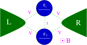
FIG. 1.: Schematic diagram of double quantum dots embedded in an Aharonov-Bohm interferometer.

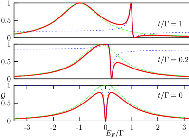
FIG. 2.: Dimensionless conductance ($\cal G$) as a function of the Fermi energy (solid lines) for three different values of the inter-dot tunneling. Other parameters are given by $\varepsilon_{1}=\varepsilon_{2}=0$, $\varphi=0.3\pi$. Long and short dashed lines denote the Breit-Wigner and the Fano asymptotes given in Eq.(20) and Eq.(21), respectively. The Fano factors for the Fano asymptotes are given by $q=0$, $q=0.423$, $q=2.115$ for $t/\Gamma=0,0.2,1$, respectively.

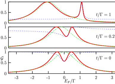
FIG. 3.: Dimensionless conductance ($\cal G$) as a function of the Fermi energy (solid lines) for three different values of the inter-dot tunneling. Other parameters are given by $\varepsilon_{1}=-0.5\Gamma$, $\varepsilon_{2}=0.5\Gamma$, $\varphi=0.3\pi$. Long and short dashed lines denote the Breit-Wigner and the generalized Fano asymptote given in Eq.(20) and Eq.(Tunable Molecular Resonances of Double Quantum Dots Embedded in an Aharonov-Bohm Interferometer), respectively. The generalized Fano factors for the asymptotes are given by $Q=0.753i$, $Q=-0.258+0.861i$, $Q=0.128+2.335i$ for $t/\Gamma=0,0.2,1$, respectively.

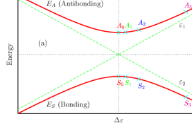
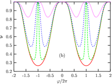
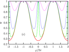
FIG. 4.: (a) Molecular two level energies as a function of the difference between the energy levels of the quantum dots. (b) AB oscillations for the bonding states marked in (a) by $S0$ (solid line), $S1$ (long-dashed line), $S2$ (short-dashed line), $S3$ (dotted line). (c) AB oscillations for the antibonding states marked in (a) by $A0$ (solid line), $A1$ (long-dashed line), $A2$ (short-dashed line), $A3$ (dotted line).

REFERENCES

- [1] M. A. Kastner, Phys. Today 46, No.1, 24 (1993).
- [2] L. P. Kouwenhoven, D. G. Austing, and S. Tarucha, Rep. Prog. Phys. 64, 701 (2001).
- [3] For a review see e.g., W. G. van der Wiel, S. De Franceschi, J. M. Elzerman, L. P. Kouwenhoven, T. Fujisawa, S. Tarucha, cond-mat/0205350.
- [4] N. C. van der Vaart et al., Phys. Rev. Lett. 74, 4702 (1995).
- [5] A. Yacoby, M. Heiblum, D. Mahalu and H. Shtrikman, Phys. Rev. Lett. 74, 4047 (1995).
- [6] R. Schuster, E. Buks, M. Heiblum, D. Mahadu, V. Umansky and H. Shtrikman, Nature 385, 417 (1997).
- [7] K. Kobayashi, H. Aikawa, S. Katsumoto, and Y. Iye, Phys. Rev. Lett. 88, 256806 (2002).
- [8] W. G. van der Wiel, S. De Franceschi, T. Fujisawa, J. M. Elzerman, S. Tarucha, and L. P. Kouwenhoven, Science 289, 2105 (2000).
- [9] Y. Ji, M. Heiblum, D. Sprinzak, D. Mahalu, and H. Shtrikman, Science 290, 779 (2000); Y. Ji, M. Heiblum, and H. Shtrikman, Phys. Rev. Lett. 88, 076601 (2002).
- [10] U. Gerland, J. von Delft, T. A. Costi, and Y. Oreg, Phys. Rev. Lett. 84, 3710 (2000).
- [11] K. Kang and S.-C. Shin, Phys. Rev. Lett 85, 5619 (2000); S. Y. Cho, K. Kang, C. K. Kim, and C.-M. Ryu, Phys. Rev. B 64, 033314 (2001); K. Kang, S. Y. Cho, and K. W. Park, Phys. Rev. B 66, 075312 (2002).
- [12] B. R. Bulka and P. Stefański, Phys. Rev. Lett. 86, 5128 (2001).
- [13] W. Hofstetter, J. König, and H. Schoeller, Phys. Rev. Lett. 87, 156803 (2001).
- [14] K. Kang and L. Craco, Phys. Rev. B 65, 033302 (2002).
- [15] A. W. Holleitner, C. R. Decker, H. Qin, K. Eberl, and R. H. Blick, Phys. Rev. Lett. 87, 256802 (2001); A. W. Holleitner, R. H. Blick, A. K. Hüttel, K. Eberl, and J. P. Kotthaus, Science 297, 70 (2002).
- [16] B. Kubala and J. König, Phys. Rev. B 65, 245301 (2002).
- [17] H. Akera, Phys. Rev. B 47, 6835 (1993).
- [18] W. Izumida, O. Sakai, and Y. Shimizu, J. Phys. Soc. Japan 66, 717 (1997).
- [19] S. Y. Cho, R. H. McKenzie, K. Kang, and C. K. Kim, cond-mat/0201487.
- [20] D. Loss and V Sukhorukov, Phys. Rev. Lett. 84, 1035 (2000).
- [21] See e.g., G. D. Mahan, Many-Particle Physics, 2nd ed. (Plenum, New York 1990).
- [22] Y. Meir and N. S. Wingreen, Phys. Rev. Lett. 68, 2512 (1992).
- [23] A. A. Clerk, X. Waintal, and P. W. Brouwer, Phys. Rev. Lett. 86, 4636 (2001).