Dynamics of a financial market index after a crash

Abstract

We discuss the statistical properties of index returns in a financial market just after a major market crash. The observed non-stationary behavior of index returns is characterized in terms of the exceedances over a given threshold. This characterization is analogous to the Omori law originally observed in geophysics. By performing numerical simulations and theoretical modelling, we show that the nonlinear behavior observed in real market crashes cannot be described by a GARCH(1,1) model. We also show that the time evolution of the Value at Risk observed just after a major crash is described by a power-law function lacking a typical scale.

I Introduction

The time evolution of basic indicators of a financial market as, for example, the volatility of a market index is often showing a non-stationary pattern Pagan . In fact, tests for whether volatility fluctuations of the size observed in empirical time series could be due to estimation error strongly reject the hypothesis of constant volatility Schwert89 .

The volatility time series, both historical and implied, experiences a dramatic increase at and immediately after each financial crash Chen . After the crash, the market volatility shows a stochastic evolution characterized by a slow decay.

A non-stationary time evolution of volatility directly implies a non-stationary time evolution of the returns of a market index. The purpose of this paper is to show that the dynamics of market index returns just after a crash presents a statistical regularity with respect to the number of times the absolute value of index return exceeds a given threshold value.

The discovered statistical regularity is analogous to a statistical law discovered in geophysics more than a century ago and known today as the Omori law Omori1894 . The Omori law states that the number of aftershock earthquakes measured at time $t$ after the main earthquake decays with $t$ as a power-law function. The observation of this specific functional form in the stochastic relaxation of the market statistical indicators to its typical values implies that the relaxation dynamics of a market index just after a financial crash is not characterized by a typical scale. The lack of a typical relaxation scale has direct implication on the estimation of risk measures as, for example, the Value at Risk of a stock portfolio Duffie97 .

The structure of the paper is as follows. In Section 2 we report on the empirical properties of aftercrash market index time series. The discussion concerns the 1-minute Standard and Poor’s 500 index returns recorded after the Black Monday financial crash. Section 3 shows that the GARCH(1,1) model is unable to describe the empirical properties of the previous section. Section 4 discusses the estimation of the Value at Risk during the time period immediately after a financial crash. The paper ends with some concluding remarks.

II Empirical properties of aftercrash sequences

In this section, we characterize the time series of ultra high frequency returns after a major market crash. The variable investigated is the one-minute logarithm changes of a financial index $r(t)$. A direct characterization of the time evolution of this random process is extremely difficult in the time period after a market crash. This is due to the fact that the aftercrash period is highly non-stationary because the financial market needs some time to be back to a ”normal” period. In order to characterize the aftercrash return time series we make use of a statistically robust method. Specifically, we quantitatively characterize the time series of index returns by investigating the number of times $|r(t)|$ is exceeding a given threshold value lillo2002 in the non-stationary time period.

A similar approach is used in the investigation of the number $n(t)$ per unit time of aftershock earthquakes above a given threshold measured at time $t$ after the main earthquake. This quantity is well described in geophysics by the Omori law Omori1894 . The Omori law $n(t)\propto t^{-p}$ says that the number of aftershock earthquakes per unit time measured at time $t$ after the main earthquake decays as a power law. In order to avoid divergence at $t=0$, Omori law is often rewritten as

$$n(t)=K(t+\tau)^{-p},$$ (1)

where $K$ and $\tau$ are two positive constants. An equivalent formulation of the Omori law, which is more suitable for comparison with real data, can be obtained by integrating Eq. (1) between $0$ and $t$. In this way the cumulative number of aftershocks after the main earthquake observed until time $t$ is

$$N(t)=K[(t+\tau)^{1-p}-\tau^{1-p}]/(1-p),$$ (2)

when $p\neq 1$ and $N(t)=K\ln(t/\tau+1)$ for $p=1$.

When the process is stationary the frequency of aftershock $n(t)$ is on average constant in time and therefore the cumulative number $N(t)$ increases linearly in time. We have tested that $N(t)$ increases approximately linearly in a market period of approximately constant volatility such as, for example, the 1984 year. For independent identically distributed random time series it is possible to characterize $n(t)$ in terms of an homogeneous Poisson process Embrechts .

As an example of the behavior of $N(t)$ empirically observed after a market crash, we investigate the index returns during the time period just after the Black Monday crash (19 October 1987) occurred at New York Stock Exchange (NYSE). This crash was one of the worst crashes occurred in the entire history of NYSE. The Standard and Poor’s 500 Index (S&P500) went down $20.4\%$ that day. In our investigation, we select a 60 trading day aftercrash time period ranging from 20 October 1987 to 14 January 1988. For the selected time period, we investigate the one-minute return time series of the S&P500 Index. The unconditional one-minute volatility is equal to $\sigma=4.91\times 10^{-4}$. In Fig. 1 we show the cumulative number of events $N(t)$ detected by considering all the occurrences observed when the the absolute value of index return exceeds a threshold value $\ell=4\sigma$. We observe a nonlinear behavior in the entire period. Fig. 1 also shows our best nonlinear fit performed with the functional form of Eq. (2). The agreement between empirical data and the functional form of the Omori law is pretty good. With a single time series it is not possible to have a good description of $n(t)$ due to the discreteness of the data. In order to solve this problem we compute $n_{av}(t)$ which is the running average of $n(t)$ in a sliding window of $200$ trading minutes. In the inset of Fig. 1 we show this quantity as a function of time in a bilogarithmic plot. A power-law behavior is observed for almost two decades and the exponent of the best power-law fit is in agreement with the exponent $p$ obtained by fitting $N(t)$.

We observe a similar behavior when we set the threshold value $\ell$ equal to $5\sigma$, $6\sigma$ and $7\sigma$. The best fit of the exponent $p$ slightly increases when $\ell$ increases and eventually converges to a constant value.

This paradigmatic behavior is not specific of the Black Monday crash of the S&P 500 index. In fact, we observe similar results also for a stock price index weighted by market capitalization for the time periods occurring after the 27 October 1997 and the 31 August 1998 stock market crashes lillo2002 . This index has been computed selecting the 30 most capitalized stocks traded in the NYSE and by using the high-frequency data of the Trade and Quote (TAQ) database issued by the NYSE.

Figure 1: Cumulative number $N(t)$ of the number of times $|r(t)|$ is exceeding the threshold $\ell=4\sigma$ during the 60 trading days immediately after the Black Monday financial crash. The parameter $\sigma$ is the standard deviation of the process $r(t)$ computed over the entire investigated period. The dashed line is the best fit of Eq. (2). The value of the exponent $p$ is 0.85. In the inset, we show $n_{av}(t)$ which is a moving average of $n(t)$ in a sliding window of 200 trading minutes. The dashed line is a power-law curve with an exponent equal to $-0.85$ and is shown as a guide for the eye

Our empirical results show that index return cannot be modeled in terms of independent identically distributed random process after a big market crash. In ref. lillo2002 we introduce a simple stochastic model which is able to explain the Omori law in financial time series. Specifically we assume that the stochastic variable $r(t)$ is the product of a deterministic time dependent scale $\gamma(t)$ times a stationary stochastic process $r_{s}(t)$ during the time period after a big crash. Under these assumptions, the number of events of $|r(t)|$ larger than $\ell$ observed at time $t$ is proportional to

$$n(t)\propto 1-F_{s}\left(\frac{\ell}{\gamma(t)}\right),$$ (3)

where $F_{s}(r_{s})$ is the cumulative distribution function of the random variable $r_{s}(t)$.

By assuming that the stationary return probability density function behaves asymptotically as a power-law

$$f_{s}(r_{s})\sim\frac{1}{r_{s}^{\alpha+1}},$$ (4)

and that the scale of the stochastic process decays as a power-law $\gamma(t)\sim t^{-\beta}$, the number of events above threshold is power-law decaying as $n(t)\sim(\gamma(t)/\ell)^{\alpha}\sim 1/t^{p}$. The exponent $p$ is given by

$$p=\alpha~{}\beta.$$ (5)

The previous relation links the exponent $p$ governing the number of events exceeding a given threshold to the $\alpha$ exponent of the stationary power-law return cumulative distribution and to the $\beta$ exponent of the power-law decaying scale.

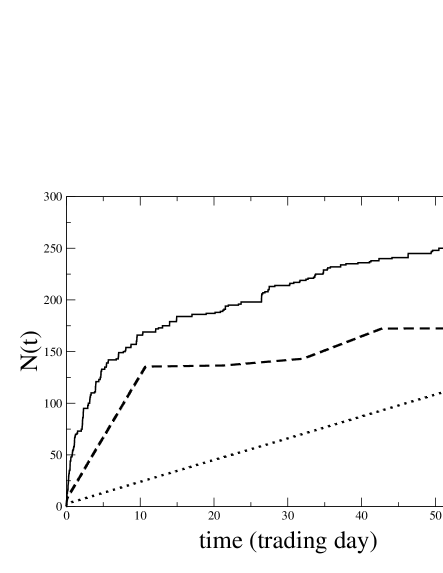
Figure 2: The dotted line is the mean value of the cumulative number $N(t)$ of the number of times $|r(t)|$ is exceeding the threshold $\ell=4\sigma$ over $10^{4}$ simulations obtained with a GARCH(1,1) model with parameters estimated in a period of 60 trading days immediately after the Black Monday financial crash. The dashed line is the mean of $N(t)$ over $10^{4}$ simulations obtained with a GARCH(1,1) model with parameters estimated in 6 nonoverlapping windows of 10 days each. As a reference we show also $N(t)$ for the real data already shown in Fig. 1 (solid line).

The hypotheses of our model are consistent with recent empirical results. In fact, a return probability density function characterized by a power-law asymptotic behavior has been observed in the price dynamics of several stocks Lux96 ; Gopi98 and a power-law or power-law log-periodic decay of implied volatility has been observed in the S&P500 after the 1987 financial crash Sornette96 . In lillo2002 we have tested the hypotheses of our model by measuring independently the exponents $\alpha$ and $\beta$ from real data and we have shown that the relation between exponents described by Eq. (5) is satisfied in all the three investigated crashes.

III Comparison with GARCH(1,1) model

Here we compare the empirical behavior of a market index after a major crash with the predictions of a simple autoregressive model, specifically the GARCH(1,1) model Bollerslev86 described by the equation

$$\sigma^{2}_{t}=\alpha_{0}+\alpha_{1}r^{2}_{t-1}+\beta_{1}\sigma^{2}_{t-1},$$ (6)

where $r_{t}$ is price return and $\sigma_{t}$ is the volatility. To this end we estimate the best value of the parameters of the GARCH(1,1) model. The estimation has been performed with the G@RCH 2.3 package garch . The best estimation of the parameters on the time series of one minute logarithmic price change during 60 trading days after Black Monday crash are $\alpha_{0}=2.87~{}10^{-8}$, $\alpha_{1}=0.38$ and $\beta_{1}=0.54$. With these parameters we generate $10^{4}$ surrogate time series according to Eq. (6) and we compute the average behavior of $N(t)$. To mimic the dynamics after the crash, we set as an initial condition a large value of return in each realization. Fig. 2 shows $N(t)$ versus time for real data and GARCH(1,1) model (dotted line) with a threshold $\ell=4\sigma$ (the same as in Fig. 1). The GARCH(1,1) time series converges to its stationary phase very quickly and it is unable to show a significant nonlinear behavior.

In order to take into account the non-stationary behavior of the return time series after a crash we have performed a different analysis. Specifically we divide the 60 trading day period in 6 nonoverlapping time intervals of 10 trading days and we estimate the GARCH(1,1) parameters specific for each interval. We then generate $10^{4}$ GARCH(1,1) surrogate time series using the estimated parameters for each subinterval. The mean value of $N(t)$ as a function of time obtained with this procedure is also shown in Fig. 2 as a dashed line. In each subinterval $N(t)$ increases linearly for almost all the period. This is due to the fact that the non-stationary part is extremely small compared with the time scale of the figure.

Below we theoretically describe the behavior of $N(t)$ expected for a GARCH(1,1) time series. First of all we note that the expectation value of $\sigma^{2}_{t}$ conditioned to the value $\sigma^{2}_{0}$ is given by Baillie92

$$E(\sigma^{2}_{t}|\sigma^{2}_{0})=\sigma^{2}_{0}(\alpha_{1}+\beta_{1})^{t}+\alpha_{0}\frac{1-(\alpha_{1}+\beta_{1})^{t}}{1-(\alpha_{1}+\beta_{1})}.$$ (7)

This equation shows that, under the assumption of finite unconditional variance $\alpha_{1}+\beta_{1}<1$, the mean value of the scale of the process decays exponentially to the unconditional value in a GARCH(1,1) time series. The decaying time is given by $\tau=-1/\ln(\alpha_{1}+\beta_{1})$. With the parameters estimated we have $\tau=12$ trading minutes in the case considered in Fig. 2.

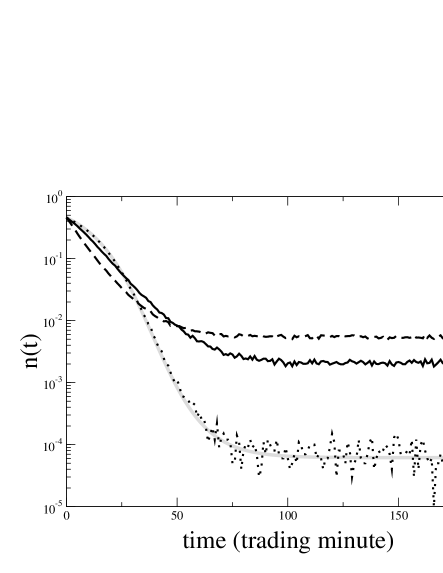
Figure 3: Mean of $n(t)$, the number per unit of time that $|r(t)|$ is exceeding the threshold $\ell=4\sigma$, for $10^{5}$ numerical simulation of three different GARCH(1,1) models with the same value of $\alpha_{0}$ and of $\alpha_{1}+\beta_{1}=0.92$. The values of $\alpha_{1}$ are $0.02$ (dotted line), $0.18$ (solid line) and $0.38$ (dashed line). This last value is the one estimated from the real time series of Black Monday aftercrash period. The gray line is the prediction based on the approximation of Gaussian density.

Since the variance of the GARCH(1,1) model depends only on $\alpha_{0}$ and on $\alpha_{1}+\beta_{1}$, we perform a set of numerical simulations of GARCH(1,1) time series with the same value of $\alpha_{0}$ and by keeping constant $\alpha_{1}+\beta_{1}=0.92$, which are the values observed in the real data. Different time series of simulations are obtained by changing the value of $\alpha_{1}$ which controls the leptokurtosis of the unconditional density. Fig. 3 shows the average of $n(t)$ over $10^{5}$ realizations of a GARCH(1,1) model with $\alpha_{1}=0.02$, $\alpha_{1}=0.18$ and $\alpha_{1}=0.38$. This last value corresponds to the one estimated from the real data. In the first two cases the unconditional kurtosis is finite, whereas for $\alpha_{1}=0.38$ the fourth moment diverges. The value of the threshold is set to $\ell=4\sigma$ in all cases. The unconditional value of $n(t)$ is larger for larger values of $\alpha_{1}$. This is expected because the unconditional densities have the same variance and the tail are fatter for larger values of $\alpha_{1}$. For all values of $\alpha_{1}$, $n(t)$ decays to the stationary value in less than a trading day. The decay is essentially exponential and a best fit with a function $n(t)=a+b~{}e^{-ct}$ gives a good agreement.

Fig. 3 also shows that the larger is $\alpha_{1}$ (and therefore the unconditional kurtosis), the faster is the decay of $n(t)$ for very small values of $t$. This empirical behavior can be modelled and hereafter we show how it is possible to find an estimate of $n(t)$ for small values of $t$. Let us consider that at time $t=0$ the crash occurs and the return is $r_{0}$. At time $t=1$ the density is Gaussian with zero mean and variance given by $\sigma_{1}=\alpha_{0}+(\alpha_{1}+\beta_{1})r_{0}^{2}$. However at subsequent times the density is no more Gaussian. As a first approximation we can assume that the density is Gaussian with time-dependent variance described by (7). This is a very rough approximation, which is valid only when $\alpha_{1}$ is very small. The gray line in Fig. 3 is $n_{gau}(t)=erfc(\ell/\sqrt{2\sigma^{2}_{t}})$ which is the function obtained by using this approximation. For large values of $t$, $n(t)$ tends to a constant value as $e^{-t/2\tau}$. The agreement is very good in the case $\alpha_{1}=0.02$. However, for larger values of $\alpha_{1}$ a better approximation is needed to explain the results of numerical simulations. A better approximation can be obtained by taking into account higher moments. Even if at time $t=1$ the density is Gaussian, at $t=2$ the density is no more Gaussian. Nevertheless we can find the exact expression for the expected value of the first four moments at $t=2$ conditioned to the information at time $t=0$. One finds

$$E_{0}(r_{2})=E_{0}(r_{2}^{3})=0,$$ (8)

$$E_{0}(r_{2}^{2})=\alpha_{0}+(\alpha_{1}+\beta_{1})\sigma_{1}^{2}\equiv s_{2}^{2},$$ (9)

$$E_{0}(r_{2}^{4})=6\alpha_{1}^{2}\sigma_{1}^{4}+E_{0}(r_{2}^{2}).$$ (10)

Under the assumption that the density is not very different from Gaussian at time $t=2$, we can approximate the density with a first order Edgeworth expansion Feller

$$p(r_{2})=\frac{e^{-r_{2}^{2}/2s_{2}^{2}}}{\sqrt{2\pi}}\left(1+He_{4}\left(\frac{r_{2}}{s_{2}}\right)\frac{\kappa_{4}(t=2)}{4!~{}s_{2}^{4}}\right),$$ (11)

where $He_{4}(x)$ is the fourth Chebyshev-Hermite polynomial and $\kappa_{4}(t)$ is the fourth cumulant of $r_{t}$. By integrating $p(x)$ in Eq. (11) between $\ell$ and infinity we can find an expression for $n(t=2)$. By performing the integration, we observe two different regimes: (i) when $\ell^{2}<3(\alpha_{0}(1+\alpha_{1}+\beta_{1})+(\alpha_{1}+\beta_{1})^{2}r_{0}^{2})$, $n(t=2)$ decreases when $\alpha_{1}$ increases; (ii) when $\ell^{2}>3(\alpha_{0}(1+\alpha_{1}+\beta_{1})+(\alpha_{1}+\beta_{1})^{2}r_{0}^{2})$, $n(t=2)$ increases when $\alpha_{1}$ increases. Table 1 shows two numerical examples corresponding to the two regimes. The results of Table 1 show that the agreement between simulated values and predicted values of $n(t)$ is quite good especially for small values of $\alpha_{1}$. The fact that for large values of $\alpha_{1}$ the agreement is less precise is due to the significant contribution coming from the moments higher than the fourth that have been neglected in the Edgeworth expansion of Eq. (11). One could improve the forecast of $n(t)$ by extending the Edgeworth expansion to higher order and by using the approximate density so obtained to calculate a better estimation of $n(t)$.

The technique of Edgeworth expansion can also be used to forecast the value of $n(t)$ for value of $t$ larger than $2$. Our numerical simulations show that for moderate values of $\alpha_{1}$ and/or short forecast horizons the predictions work quite well. For larger value of $\alpha_{1}$ (especially when the fourth moment of the unconditional density is infinite) the prediction is valid only for small values of $t$.

These theoretical and numerical observations confirm that the GARCH(1,1) is unable to model the power law decay of $n(t)$ observed in real time series after a major market crash.

Table 1: Simulated and theoretical values of $n(t=2)$ in a GARCH(1,1,) model for different values of $\alpha_{1}$ and for the two regimes described in the text. Case (i) corresponds to $r_{0}=3.4~{}10^{-3}$ and case (ii) corresponds to $r_{0}=1~{}10^{-3}$. The other parameters are: $\alpha_{0}=2.87~{}10^{-8}$, $\ell=4\sigma=2.4~{}10^{-3}$.

		case (i)		case (ii)
$\alpha_{1}$	$\beta_{1}$	$n_{sim}(2)$	$n_{teo}(2)$	$n_{sim}(2)$	$n_{teo}(2)$
0.02	0.90	$4.41~{}10^{-1}$	$4.41~{}10^{-1}$	$1.11~{}10^{-2}$	$1.15~{}10^{-2}$
0.18	0.74	$4.34~{}10^{-1}$	$4.31~{}10^{-1}$	$1.26~{}10^{-2}$	$1.40~{}10^{-2}$
0.38	0.54	$4.11~{}10^{-1}$	$3.95~{}10^{-1}$	$1.75~{}10^{-2}$	$2.26~{}10^{-2}$
0.58	0.34	$3.73~{}10^{-1}$	$3.33~{}10^{-1}$	$2.27~{}10^{-2}$	$3.75~{}10^{-2}$

IV Value at Risk after a crash

The empirical evidence and the theoretical model shown in the previous sections have direct relevance for risk management. One of the most widely used measure of risk is the so called Value at Risk (VaR) Duffie97 . The VaR is the most probable worst expected loss at a given level of confidence over a given time horizon. Here we indicate the probability density for index return $r$ over the time horizon $\tau$ as $f_{\tau}(r)$. The VaR $\Lambda_{VaR}$ associated to a certain probability of loss $P_{VaR}$ is defined implicitly by

$$\int_{-\infty}^{-\Lambda_{VaR}}f_{\tau}(r)~{}dr=P_{VaR}.$$ (12)

In stationary market conditions, the VaR is determined by the the density $f_{\tau}(r)$. In Section 2 we have discussed a simple market model able to describe quantitatively the non-stationary evolution of index return time series after a market crash. In this model the shape of the return density remains constant but its scale changes in time. By using the relation $r(t)=\gamma(t)r_{s}(t)$, it is direct to show that the (instantaneous) VaR after a market crash is not constant but changes in time as

$$\Lambda_{VaR}(t)=\gamma(t)\Lambda^{(s)}_{VaR},$$ (13)

where $\Lambda^{(s)}_{VaR}$ is the constant VaR obtained by using the stationary probability density function $f_{s}(r_{s})$. We have seen lillo2002 that the occurrence of the Omori law after a market crash is consistent with a time evolution of the scale $\gamma(t)=c_{1}t^{-\beta}+c_{2}$. Eq. (13) indicates that after a big market crash the VaR decreases in time as a power-law with exponent $\beta$ (close to $0.2\div 0.3$ in the investigated crashes) and eventually relaxes to a constant value.

V Conclusions

Our empirical observations show that the statistical properties of index return time series after a major financial crash are essentially different from the ones observed far from the crash. Other examples of statistical properties of market which are specific of the aftercrash period have been observed in the investigation of cross-sectional quantities computed for a set of stocks before, at and after financial crashes Lillo2000 ; Lillo2001 . The time period just after a crash is characterized by a relaxation to the typical market phase that can be modelled in terms of a power-law decay of the typical scale of index returns. We have shown that this observation rules out the possibility that the statistical properties of the time evolution of index returns can be efficiently modelled in terms of simple autoregressive models, such as the GARCH(1,1) model, in the non-stationary period after a crash. Our modelling of the aftercrash period also suggests that the Value at Risk of a financial portfolio measured just after a financial crash evolves in a non trivial way characterized by a power-law evolution lacking a typical scale. In summary we conclude that the time period after a major market crash is characterized by statistical regularities which are specific to such a time period and not well described by models which presents a typical time scale in their stochastic evolution. The authors thank INFM ASI and MURST for financial support.

- (1) Pagan, A., 1996. The econometrics of financial markets. Journal of Empirical Finance. 3, 15-102.
- (2) Schwert, G.W., 1989. Why Does Stock Market Volatility Change Over Time? The Journal of Finance. 44, 1115-1153.
- (3) Chen, N.-F., Cuny, C.J., Haugen, R.A., 1995. Stock Volatility and the Levels of the Basis and Open Interest in Futures Contracts. The Journal of Finance. 50, 281-300.
- (4) Omori, F., 1894. On the after-shocks of earthquakes. J. Coll. Sci. Imp. Univ. Tokyo 7, 111-200.
- (5) Duffie, D., Pan, J., 1997. An overview of Value at Risk. Journal of Derivatives. 4, 7-49.
- (6) Lillo, F., Mantegna, R.N., 2001. Power-law relaxation in a complex system: The fluctuation decay after a financial market crash. http://xxx.lanl.gov/abs/cond-mat/0111257.
- (7) Embrechts, P., Klüppelberg, C., Mikosch, T., 1997. Modelling Extremal Events for Insurance and Finance. Springer-Verlag, Berlin Heidelberg.
- (8) Lux, T., 1996. The stable Paretian hypothesis and the frequency of large returns: an examination of major German stocks. Applied Financial Economics 6, 463-475.
- (9) Gopikrishnan, P., Meyer, M., Amaral, L.A.N., Stanley, H.E., 1998. Inverse Cubic Law for the Distribution of Stock Price Variations. European Physical Journal B 3, 139-140.
- (10) Sornette, D., Johansen, A., Bouchaud, J.-P., 1996. Stock Market Crashes, Precursors and Replicas. Journal de Physique France 6, 167-175.
- (11) Bollerslev, T., 1986. Generalized Autoregressive Conditional Heteroskedasticity. Journal of Econometrics 31, 307-327.
- (12) Information and the package can be dowloaded at the web site http://www.egss.ulg.ac.be/garch/.
- (13) Baillie, R.T., Bollerslev, T., 1992. Prediction in dynamic models with time-dependent coditional variances. Journal of Econometrics. 52, 91-113.
- (14) Feller, W. 1971. An Introduction to Probability and Its Application, Vol.2. J. Wiley & Sons, New York.
- (15) Lillo, F., Mantegna, R.N., 2000. Symmetry alteration of ensemble return distribution in crash and rally days of financial markets. European Physical Journal B 15, 603-606.
- (16) Lillo, F., Mantegna, R.N., 2001. Empirical properties of the variety of a financial portfolio and the single-index model. European Physical Journal B 20, 503-509.