Phase diagrams of spin ladders with ferromagnetic legs

I Introduction

A theoretical understanding of the properties of quantum spin ladder systems has attracted a lot of current interest for a number of reasons: on the one hand there is an increasing number of new magnetic materials with a ladder-like structure characterized by rich ground state phase diagrams [1]. On the other hand, spin-ladder models pose interesting theoretical problems. For example, since a spin-$S$ chain can be described as a $2S$-leg ladder with spin $S=1/2$, provided the interchain coupling is appropriately chosen [2, 3, 4] the even- or odd-leg ladder systems are an excellent demonstration for Haldane’s conjecture [6] as generalized to $S=1/2$ ladders: the antiferromagnetic spin ladder with an even number of legs corresponds to a spin chain with integer spin and is predicted to have a gap, while a ladder with odd number of legs has a gapless excitation spectrum. The two-leg antiferromagnetic ladder is presumably the simplest spin system which allows to follow the continuous evolution between spin $S=1/2$ and $S=1$ antiferromagnetic chains nearly exactly [4, 5].

The two-leg ladder model has been the subject of considerable theoretical interest [7, 8, 9, 10, 11, 12, 13, 14, 15, 16, 17, 18, 19, 20, 21, 22, 23, 24, 25, 26, 27, 28, 29, 30, 31, 32, 33, 34, 35], most of this work, however, concentrated on isotropic or weakly anisotropic antiferromagnetic chains coupled by an interchain exchange of arbitrary sign. Ladder systems with ferromagnetic legs are much less studied although, as will be shown here they exhibit new interesting aspects. The ferromagnetic ladder model in the vicinity of the ferromagnetic instability point was recently studied by Kolezhuk and Mikeska within the framework of quasiclassical analysis based on a nonlinear $\sigma$-model approach [24]. In this work we extend these studies addressing the problem of ref. [24] in the extreme quantum limit of spins 1/2 and investigate the weak-coupling ground state phase diagram of a $S=1/2$ ladder system with ferromagnetic legs and anisotropic interleg exchange using the continuum limit bosonization approach.

The Hamiltonian of the model under consideration is given by

$$\hat{H}=H_{leg}^{1}+H_{leg}^{2}+H_{\perp}\,,$$ (1)

where the Hamiltonian for leg $\alpha$ is

$$H_{leg}^{\alpha} = -J\sum_{j=1}^{N}\big{(}S^{x}_{\alpha,j}S^{x}_{\alpha,j+1}+S^{y}_{\alpha,j}S^{y}_{\alpha,j+1}$$ (2)

$$+ \Delta\,S^{z}_{\alpha,j}S^{z}_{\alpha,j+1}\big{)}\,,$$ (3)

and the interleg coupling is given by

$$H_{\bot} = J^{xy}_{\bot}\sum_{j=1}^{N}\left(S^{x}_{1,j}S^{x}_{2,j}+S^{y}_{1,j}S^{y}_{2,j}\right)$$ (4)

$$+ J^{z}_{\bot}\sum_{j=1}^{N}S^{z}_{1,j}S^{z}_{2,j}\,.$$ (5)

Here $S^{x,y,z}_{\alpha,j}$ are spin $S=1/2$ operators at the $j$-th rung, the index $\alpha=1,2$ denotes the ladder legs. The intraleg coupling constant is ferromagnetic, $J>0$, and therefore the limiting case of isotropic ferromagnetic legs corresponds to ${\Delta}=1$, while the case of isotropic antiferromagnetic legs is obtained for ${\Delta}=-1$. Since we study the ground state phase diagram of the ladder system with ferromagnetic legs we will restrict ourselves to consider ${\Delta}>0$, including $|{\Delta}|\ll 1$ in the limit of legs with strong in-plane anisotropy.

The outline of the paper is as follows: In section II we derive the bosonized formulation of the model in the continuum limit. In section III we discuss the weak coupling phase diagrams of the model for three different cases of anisotropic interleg coupling. Finally, we conclude and summarize our results in section IV. In the appendix we present the spin-wave approach to study the transition line related to the ferromagnetic instability in the system.

II Bosonization

In this section we derive the low-energy effective field theory of the lattice model Eq. (1). Since the weak-coupling bosonization approach to the ladder models is based on the perturbative treatment of the interchain couplings [12, 4] we start from the bosonization of separate spin $S=1/2$ ferromagnetic $XXZ$ chains.

A Separate chains

The anisotropic spin $S=1/2$ Heisenberg chain with $|\Delta|<1$ is known to be critical. The long wavelength excitations are described by the standard gaussian theory [36] with hamiltonian

$${\cal H}_{leg}={u\over 2}\int dx\,[(\partial_{x}\phi)^{2}+(\partial_{x}\theta)^{2}].$$ (6)

$\phi(x)$ and $\theta(x)$ are dual bosonic fields, $\partial_{t}\phi=u\partial_{x}\theta$, and satisfy the following commutational relation

$$[\phi(x),\theta(y)]=i\Theta(y-x)\,,$$ (7)

$$[\phi(x),\theta(x)]=i/2\,.$$ (8)

$u$ stands for the velocity of spin excitation and is fixed from the Bethe ansatz solution as [36]

$$u = J\frac{K}{2K-1}\sin{\left(\pi/2K\right)}\,,$$ (9)

where $K$ is Luttinger liquid parameter known from comparison with the exact solution of the $XXZ$ chain:

$$K = \frac{\pi}{2\arccos\Delta}\,.$$ (10)

Thus the parameter $K$ increases monotonically along the $XXZ$ critical line $-1<\Delta<1$ from its minimal value $K=1/2$ at $\Delta=-1$ (isotropic antiferromagnetic chain), is equal to unity at $\Delta=0$ (the $XY$ chain) and $K\to\infty$ at $\Delta\to 1$. At $\Delta=1$ the spin excitation velocity vanishes, $u=0$. This corresponds to the ferromagnetic instability point of a single chain.

To obtain the bosonized version of the ladder Hamiltonian we need the explicit bosonized expressions of the spin operators. The bosonization procedure for the spin $S=1/2$ Heisenberg chain is reviewed in many places [37, 38, 39]. However, since we consider the ladder model with ferromagnetic legs, our bosonization conventions require some comments. The unitary transformation

$$S_{\alpha,j}^{x,y}\rightarrow(-1)^{j}S_{\alpha,j}^{x,y}\,,\quad S_{\alpha,j}^{z}\rightarrow S_{\alpha,j}^{z}\,$$ (11)

changes the sign of the intrachain transverse exchange and maps the Hamiltonian  (1) to the Hamiltonian with antiferromagnetic legs. To maintain the ferromagnetic character of the in-plane correlations in the bosonization, it is convenient to implement the multiplicative factor $(-1)^{j}$, introduced by the unitary transformation  (11), directly in the bosonized expressions for the transverse components of the spin operators. Using the standard bosonization formulas [37, 38, 39] we obtain:

$$S_{j,\alpha}^{x} \simeq \frac{{\it c}}{\sqrt{2\pi}}:\cos\sqrt{\frac{\pi}{K}}\theta_{\alpha}:\,$$ (12)

$$+ (-1)^{j} \,\frac{{\it ib}}{\sqrt{2\pi}}:\sin\sqrt{4\pi K}\phi_{\alpha}\sin\sqrt{\frac{\pi}{K}}\theta_{\alpha}:\,,$$ (13)

$$S_{j,\alpha}^{y} \simeq \frac{{\it c}}{\sqrt{2\pi}}:\sin\sqrt{\frac{\pi}{K}}\theta_{\alpha}:\,$$ (14)

$$- (-1)^{j} \,\frac{{\it ib}}{\sqrt{2\pi}}:\sin\sqrt{4\pi K}\phi_{\alpha}\cos\sqrt{\frac{\pi}{K}}\theta_{\alpha}:\,,$$ (15)

$$S_{j,\alpha}^{z} = \sqrt{\frac{K}{\pi}}\partial_{x}\phi_{\alpha}\,+$$ (16)

$$(-1)^{j} \,\frac{{\it a}}{\pi}:\sin\sqrt{4\pi K}\phi_{\alpha}(x):\,.$$ (17)

Note that the first and the second terms in Eqs. (13),(15) are hermitian because of (7). Furthermore $:...:$ denotes the normal ordering with respect to free bose system (6), $\alpha$ is the leg index. The non-universal real constants a, b and c depend smoothly on the parameter $\Delta$, are of the order of unity at $\Delta=0$ [40, 41] and are expected to be nonzero at arbitrary $\Delta<1$.

B Coupled Spin-1/2 Chains

For coupled $S=1/2$ chains we start with two critical $S=1/2$ Heisenberg chains and treat the interleg coupling as a perturbation assuming $|J^{z}_{\bot}|,|J^{xy}_{\bot}|\ll J$. Therefore we start with two free bose field Hamiltonians (6) and simply attach a leg index $\alpha=1,2$ to the fields.

Then we introduce the symmetric and antisymmetric combinations of the bosonic fields:

$$\phi_{\pm}=\sqrt{\frac{1}{2{\Lambda_{\pm}}}}\left(\phi_{1}\pm\phi_{2}\right)\,,\theta_{\pm}=\sqrt{\frac{{\Lambda_{\pm}}}{2}}\left(\theta_{1}\pm\theta_{2}\right),$$ (18)

where

$$\Lambda_{\pm}=\left(1\mp\frac{1}{2\pi}\frac{J^{z}_{\bot}}{J_{eff}}\right)$$

and

$$J_{eff}=J\frac{1}{2K-1}\sin{\frac{\pi}{2K}}\,.$$

Using Eqs. (13)-(17), we finally obtain the following bosonic Hamiltonian density:

$${\cal H} = {\cal H}^{+}+{\cal H}^{-}+{\cal H}^{\pm}_{int}\,,$$ (19)

$${\cal H}^{+} = {u_{+}\over 2}[(\partial_{x}\theta_{+})^{2}+(\partial_{x}\phi_{+})^{2}]$$ (20)

$$- \frac{{\cal J}_{\bot}^{z}}{2\pi}\cos{\sqrt{8\pi K_{+}}\phi_{+}(x)}\,,$$ (21)

$${\cal H}^{-} = {u_{-}\over 2}[(\partial_{x}\theta_{-})^{2}+(\partial_{x}\phi_{-}(x))^{2}]$$ (22)

$$+ \frac{{\cal J}_{\bot}^{z}}{2\pi}\cos{\sqrt{8\pi K_{-}}\phi_{-}(x)}$$ (23)

$$+ \frac{{\cal J}_{\bot}^{xy}}{2\pi}\cos{\sqrt{\frac{2\pi}{K_{-}}}\theta_{-}(x)}\,,$$ (24)

$${\cal H}^{\pm}_{int} = \frac{{\cal J}_{+-}}{2\pi}\,\cos{\sqrt{\frac{2\pi}{K_{-}}}\theta_{-}(x)}\cos{\sqrt{8\pi K_{+}}\phi_{+}(x)}\,.\$$ (25)

Here

$$u_{\pm} = \frac{u}{\Lambda_{\pm}}\simeq u\left(1\pm\frac{1}{2\pi}\frac{J^{z}_{\bot}}{J_{eff}}\right)$$ (26)

$$K_{\pm} = K\cdot\Lambda_{\pm}\simeq K\left(1\mp\frac{1}{2\pi}\frac{J^{z}_{\bot}}{J_{eff}}\right)\,,$$ (27)

and we have introduced the following coupling constants:

$${\cal J}_{\bot}^{z}=J_{\bot}^{z}/\pi\,,$$ (28)

for $\Delta=0$ and otherwise

$${\cal J}_{\bot}^{z} \sim J_{\bot}^{z}\,,$$ (29)

$${\cal J}_{\bot}^{xy},{\cal J}_{+-} \sim J_{\bot}^{xy}\,,$$ (30)

with some positive constants of proportionality which cannot be fixed by symmetry arguments (contrary to the constant appearing in Eq. (28)).

In deriving (19), a term $\sim\cos{\sqrt{\frac{2\pi}{K_{-}}}\theta_{-}}\cos{\sqrt{8\pi K_{-}}\phi_{-}}$ which is strongly irrelevant at $\Delta>0$ (ferromagnetic legs) was omitted. Thus our approach is tailored to cover ferromagnetic intraleg coupling and can be applied to antiferromagnetic intraleg coupling only for $|\Delta|\ll 1$.

C The effective continuum-limit model

At $J^{z}_{\bot}=J^{xy}_{\bot}=0$ the Hamiltonian (19) describes two independent Gaussian fields, i.e. two gapless fields, each describing a critical spin S=1/2 Heisenberg chain. Let us first address the question whether the interleg exchange leads to the dynamical generation of a gap in the excitation spectrum. In the case of anisotropic interleg exchange it is rather instructive to study the effect of the longitudinal ($J_{\bot}^{z}$) and transverse ($J_{\bot}^{xy}$) part of the interleg coupling separately.

At $J_{\bot}^{xy}=0$ the effective theory of the original ladder model is given by two decoupled quantum sine-Gordon models

$${\cal H}_{eff}={\cal H}^{+}+{\cal H}^{-}$$ (31)

where

$${\cal H}^{\pm} = u_{\pm}\int dx\,\Big{[}{1\over 2}[(\partial_{x}\theta_{\pm}(x))^{2}+(\partial_{x}\phi_{\pm}(x))^{2}]$$ (32)

$$+ {M_{\pm}\over 2\pi}\cos{\sqrt{8\pi K_{\pm}}\phi_{\pm}(x)}\Big{]}\,.$$ (33)

The two SG models respectively describe the symmetric ($\phi_{+}$) and antisymmetric ($\phi_{-}$) degrees of freedom.

The bare values of the dimensionless coupling constants $M_{\pm}$ and $K_{\pm}$ are known only in the weak-coupling limit $|J_{\bot}^{z}|/J,|\Delta|\ll 1$ where they have the values:

$$M_{\pm} = \mp{J_{\bot}^{z}\over\pi J}\,,$$ (34)

$$K_{\pm} = 1+\frac{2\Delta}{\pi}\mp\frac{J_{\bot}^{z}}{2\pi J}\,.$$ (35)

The scaling dimensions of the cosine terms in (32) are $d^{z}_{\pm}=2K_{\pm}\simeq 2$. Therefore, in the weak-coupling limit, both SG models have marginal dimension and details of their behavior should be determined within the framework of the renormalization-group analysis. However, a rather straightforward estimate indicates that at $\Delta\gg 4J_{\bot}^{z}/J$ we have $K_{\pm}>1$ and the cosine terms are irrelevant. Therefore in this case one concludes that the effective model reduces to the theory of two independent Gaussian fields $\phi_{\pm}$. The effect of the interleg coupling is extremely weak and is completely absorbed in the renormalized values of the spin-liquid parameters $K_{\pm}$ characterizing respectively gapless symmetric and antisymmetric modes. However, it is important to note, that in the vicinity of the single chain ferromagnetic instability point, at $\Delta\to 1$, the effective bandwidth collapses, $J_{eff}\simeq 2(1-\Delta)\to 0$. Therefore in this limit the effect of the interleg coupling becomes very strong. This implies subtle effects to be discussed later.

The transverse interleg exchange ($J_{\bot}^{xy}$) leads to the appearance of the strongly relevant operator ${\cal J}_{\bot}^{xy}\cos{\sqrt{2\pi K^{-1}_{-}}\theta_{-}}$ with the scaling dimension $d^{xy}_{-}=(2K_{-})^{-1}\leq 1/2$ in the theory. Therefore, the antisymmetric sector is gapped at arbitrary $J_{\bot}^{xy}\neq 0$. Fluctuations of the field $\theta_{-}(x)$ are completely suppressed in this sector and $\theta_{-}(x)$ is condensed in one of its vacua. The vacuum expectation value of the cosine term is

$$\langle\cos{\sqrt{2\pi K^{-1}_{-}}\theta_{-}}\rangle=\gamma$$ (36)

with $\gamma\sim\left(|{\cal J}_{\bot}^{xy}|/J_{eff}\right)^{\frac{d^{xy}_{-}}{2-d^{xy}_{-}}}\ll 1$ in weak coupling and is of the order of unity at $|{\cal J}_{\bot}^{xy}|\geq J$.

Therefore, the condensation of the field $\theta_{-}$ strongly influences the coupling between the symmetric and antisymmetric modes induces by ${\cal H}^{\pm}_{int}$. Taking into account that the fluctuations of the field $\theta_{-}$ are stopped, one easily finds that at $J_{\bot}^{xy}\neq 0$ infrared behavior of the symmetric field is governed by the following ”effective” sine-Gordon theory

$${\cal H}^{+}_{eff} = u_{+}\int dx\,\Big{[}{1\over 2}[(\partial_{x}\theta_{+})^{2}+(\partial_{x}\phi_{+}(x))^{2}]$$ (37)

$$+ {M^{+}_{eff}\over 2\pi}\cos{\sqrt{8\pi K_{+}}\phi_{+}(x)}\Big{]}\,,$$ (38)

where

$$M^{+}_{eff}=-\frac{1}{\pi u_{+}}\left({\cal J}^{z}_{\bot}+\gamma\cdot|{\cal J}_{+-}|\right)\,.$$ (39)

This mapping of the initial spin $S=1/2$ ladder model onto the quantum theory of Bose fields described in terms of an ”effective” sine-Gordon (SG) Hamiltonian (32) or (37) will allow to extract the ground state properties of the $S=1/2$ ladder using the far-infrared properties of the quantum SG theory.

D The RG analysis

The infrared behavior of the SG Hamiltonian is described by the corresponding pair of renormalization group (RG) equations for the effective coupling constants ${\cal K}(l)$ and ${\cal M}(l)$

$$\frac{d{\cal M}(l)}{dl} = -2\left({\cal K}(l)-1\right){\cal M}(l)$$ (40)

$$\frac{d{\cal K}(l)}{dl} = -\frac{1}{2}{\cal M}^{2}(l)$$ (41)

where $l=\ln(a_{0})$ and the bare values of the coupling constants are ${\cal K}(l=0)\equiv K$ and ${\cal M}(l=0)\equiv M$. The pair of RG equations (40) describes the Kosterlitz-Thouless transition [42]. The flow lines lie on the hyperbola

$$4\left({\cal K}-1\right)^{2}-{\cal M}^{2}=\mu^{2}=4(K-1)^{2}-M^{2}$$ (42)

and exhibit two different regimes depending on the relation between the bare coupling constants - [43] (see Fig.1):

FIG. 1.: Renormalization-group flow diagram; the arrows denote the direction of flow with increasing length scale.

Weak coupling regime.   For $2(K-1)\geq\left|M\right|$ we are in the weak coupling regime: the effective mass ${\cal M}\to 0$. The low energy (large distance) behavior of the corresponding gapless mode is described by a free scalar field.

The vacuum averages of exponentials of the corresponding fields show a power-law decay at large distances

$$\langle\,e^{iK\phi(0)}\,e^{-iK\phi(r)}\rangle\sim\langle\,e^{iK\theta(0)}\,e^{-iK\theta(r)}\rangle\sim\left|r\right|^{-\frac{K^{*2}}{2\pi}}\,.$$ (43)

where $K^{\ast}$ is the fixed-point value of the parameter $K$ determined from the Eq. (42).

Strong coupling regime.   For $2(K-1)<\left|M\right|$ the system scales to strong coupling: depending on the sign of the bare mass $M$, the renormalized mass ${\cal M}$ is driven to $\pm\infty$, signaling a crossover to one of two strong coupling regimes with a dynamical generation of a commensurability gap in the excitation spectrum. The flow of $\mid{\cal M}\mid$ to large values indicates that the ${\cal M}\mbox{cos}\sqrt{8\pi K}\phi$ term in the sine-Gordon model dominates the long-distance properties of the system. Depending on the sign of the mass term, the field $\phi$ gets ordered with the expectation values

$$\langle\phi\rangle=\left\{\begin{array}[]{ll}\sqrt{\pi/8K}\hskip 14.22636pt\textrm{ at $M>0$}\\ 0\hskip 42.67912pt\textrm{ at $M<0$}\end{array}\right.\,.$$ (44)

Using this analysis for the excitation spectrum of the SG model and the behavior of the corresponding fields, Eqs. (43, 44), we will now discuss the weak-coupling phase diagram of the spin $S=1/2$ ferromagnetic ladder model Eq. (1).

III Phase diagrams

In this section we discuss separately the ground state phase diagram of the ferromagnetic ladder coupled only by the longitudinal part of the interleg spin exchange (subsection A), coupled only by the transverse part of the interleg spin exchange (subsection B) and by an isotropic interleg coupling (subsection C). At this point we note that from the structure of the interaction Hamiltonian Eq. (4) follows that the phase diagrams for case (A) and case (B) will be symmetric with respect to the lines $J_{\perp}=0$ since a change of sign in $J_{\perp}$ leads to a unitary equivalent Hamiltonian. This is in contrast to case (C) where this unitary equivalence does not exist.

A Chains coupled by the longitudinal part of the interleg exchange

In this subsection we consider the weak-coupling phase diagram of the spin S=1/2 ferromagnetic ladder model  (1) coupled by a weak longitudinal intrachain exchange ($J^{xy}_{\bot}=0,J^{z}_{\bot}\neq 0$). The bosonized version of the model ${\cal H}_{eff}={\cal H}^{+}+{\cal H}^{-}$ where ${\cal H}^{\pm}$ are given by Eq. (32) and the bare values of the corresponding dimensionless coupling constants are given by (34)-(35). By inspection of the initial values of the coupling constants one easily finds that:

• At $\Delta<0$ both the symmetric and the antisymmetric sectors are gapped (except for $J_{\bot}^{z}=0)$.

• At $\Delta>0$ the symmetric sector is gapped for $J_{\bot}^{z}/J>2\Delta>0$ while the antisymmetric sector is gapped for $J_{\bot}^{z}/J<-2\Delta<0$.

This determines the following three distinct sectors of the phase diagram as traced already in the RG analysis (see also Fig. 2 below):

• Sector A: $\Delta<0$ corresponds to the phase with gapped excitation spectrum;

• Sector B: $\Delta>0$ and $|J_{\bot}^{z}|>2J\Delta$ corresponds to the phase characterized by the one gapless and one gapped mode in the excitation spectrum. In particular at $J_{\bot}^{z}>0$ the symmetric mode is gapped whereas the antisymmetric mode is gapless and vice-versa at $J_{\bot}^{z}<0$;

• Sector C: $\Delta>0$ and $|J_{\bot}^{z}|<2J\Delta$ corresponds to the phase where both modes are gapless.

As we show below, the same phases are present in the strong coupling regime. The only phase which is missed in the weak-coupling RG analysis is the ferromagnetic phase; it appears only in the strong coupling regime at $\Delta\simeq 1$ or at $\Delta\ll 1$ but $|J_{\bot}^{z}|\sim 1/\Delta\gg 1$.

To clarify the symmetry properties of the ground states of the system in the different sectors we study the large-distance behavior of the longitudinal

$$K^{zz}_{\alpha\beta}(r):=\langle S_{\alpha}^{z}(0)S_{\beta}^{z}(r)\rangle\,,$$ (45)

and the transverse

$$K^{xy}_{\alpha\beta}(r):=\langle S_{\alpha}^{+}(0)S_{\beta}^{-}(r)\rangle\,,$$ (46)

spin-spin correlation functions for intraleg ($\alpha=\beta$) and interleg ($\alpha\neq\beta$) spin pairs.

Using the results for the excitation spectrum and the behavior of the corresponding fields in the gapless and gapped phases, Eqs. (43)-(44), and the expressions for the corresponding correlation functions from bosonization, we now discuss the characteristics of the various phases in the different sectors of the weak-coupling ground state phase diagram.

In the sector A ($J^{z}_{\bot}<0$) the vacuum expectation values of the fields are: $\langle\phi_{+}\rangle=\sqrt{\displaystyle{\pi/8K_{+}}}$ and $\langle\phi_{-}\rangle=0$. Ordering of the $\phi_{\pm}$ suppresses transverse spin correlations, while the longitudinal correlations are given by

$$K^{zz}_{\alpha\beta}(r)\sim(-1)^{r}\,\cdot\mbox{\it constant}\,.$$

Therefore at $\Delta<0$ and $J_{\bot}^{z}<0$, the long-range ordered (LRO) antiferromagnetic phase with inphase spin ordering on the rungs is realized in the ground state of the system.

In the Sector A1 ($J^{z}_{\bot}<0$) the vacuum expectation values of the fields are given by $\langle\phi_{+}\rangle=0$ and $\langle\phi_{-}\rangle=\sqrt{\displaystyle{\pi/8K_{-}}}$. This immediately implies that in this sector

$$K^{zz}_{\alpha\beta}(r)\sim(-1)^{\alpha+\beta}\cdot(-1)^{r}\,\cdot\mbox{\it constant}\,.$$

Therefore, at $\Delta<0$ and $J_{\bot}^{z}>0$ the LRO antiferromagnetic phase with antiphase intrarung spin ordering is realized in the ground state of the system.

In the sector B (B1) the antisymmetric (symmetric) field is gapped with the vacuum expectation value $\langle\phi_{-}\rangle=0$ ($\langle\phi_{+}\rangle=0$). However, as can be seen from weak coupling RG analysis as well as from the strong coupling effective spin $1/2$ model (see below), at $J^{z}_{\bot}\neq 0$ the line $\Delta=0$ is the phase transition line along which the gapped at $\Delta<0$ symmetric (antisymmetric) mode becomes gapless. Therefore in the sector B (B1) the gapless degrees of freedom corresponding to the symmetric (antisymmetric) mode are described by the free Bose field system with the fixed-point value of the parameters $K^{\ast}_{\pm}$. Using Eq. (42) and the bare values of coupling constants (34)-(35) it is straightforward to show that at $|\Delta|,|J^{z}_{\bot}/J|\ll 1$

$$K^{\ast}_{\pm}\simeq 1+\frac{1}{\pi}\sqrt{2\Delta(2\Delta\mp J^{z}_{\bot}/J)}\,.$$

Note that at $\Delta=0$ the fixed-point values of the spin-liquid parameters are $K^{\ast}_{\pm}=1$ while at $J^{z}_{\bot}=0$ (see Eq. (27)) $K^{\ast}_{\pm}=K$. Therefore we conclude that along the line $\Delta=0$ the gapless sector in the system is identical to a single isotropic spin $S=1/2$ Heisenberg chain, while along the line $J^{z}_{\bot}=0$ we reach the limit of two decoupled spin $S=1/2$ Heisenberg chains.

The very existence of a gapped excitation mode accompanied with ordering of the field $\phi_{-}$ (or $\phi_{+}$) implies suppression of the transverse correlations. On the other hand the presence of the gapless excitation mode leads to the power law decay of the longitudinal spin correlations. Therefore we obtain, that in the sector B

$$K^{zz}_{\alpha\beta}(r)\simeq\frac{K^{\ast}_{+}}{2\pi r^{2}}+\frac{(-1)^{r}}{r^{K^{\ast}_{+}}}\,,$$

while in the sector B1

$$K^{zz}_{\alpha\beta}(r)\simeq(-1)^{\alpha+\beta}\,\left[\frac{K^{\ast}_{-}}{2\pi r^{2}}+\frac{(-1)^{r}}{r^{K^{\ast}_{-}}}\right]\,.$$

We denote this phase as the spin liquid I phase. It is interesting to note that in sector B the following operator shows quasi long range behavior:

$$\langle(S_{1}^{+}(r) + S_{2}^{+}(r))^{2}\,(S_{1}^{-}(0)+S_{2}^{-}(0))^{2}\rangle$$ (47)

$$\simeq 4\langle S_{1}^{+}(r)S_{2}^{+}(r))\,S_{1}^{-}(0)S_{2}^{-}(0)\rangle$$ (48)

$$\simeq r^{-1/K_{+}^{*}}\,\,(-1)^{r}\,r^{-1/K_{+}^{*}-K_{+}^{*}}.$$ (49)

$(S_{1}^{\alpha}+S_{2}^{\alpha})^{2}$ for the $S=\frac{1}{2}$ ladder corresponds to the operator $(S^{\alpha})^{2}$ in the $S=1$ chain and we therefore identify sector B with the $XY2$ phase for the $S=1$ chain as described in ref.[[2]].

With increasing interleg ferromagnetic coupling we reach the line $\Delta=|J_{\bot}^{z}|/2J$ which marks the transition into the phase where both fields are gapless. In the sector C of the phase diagram the system shows properties of two almost independent spin $S=1/2$ anisotropic Heisenberg chains with dominating ferromagnetic coupling. The transverse correlations in this phase are given by

$$K^{xy}_{\alpha\beta}(r) \simeq \delta_{\alpha\beta}\Big{[}r^{-1/4(1/K^{\ast}_{+}+1/K^{\ast}_{-})}$$ (50)

$$+ (-1)^{r}\cdot r^{-\left(K^{\ast}_{+}+K^{\ast}_{-}+1/4K^{\ast}_{+}+1/4K^{\ast}_{-}\,\right)}\Big{]},$$ (51)

where $\delta_{\alpha,\beta}$ is the Kronecker symbol. The longitudinal correlations decay faster. In particular the intraleg longitudinal correlations are given by

$$K^{zz}_{\alpha\alpha}(r)\simeq\frac{K^{\ast}_{+}+K^{\ast}_{-}}{2\pi r^{2}}+(-1)^{r}\cdot\,r^{-\left(K^{\ast}_{+}+K^{\ast}_{-}\right)}\,.$$ (52)

The transverse interleg correlations are strongly suppressed in this phase, while the longitudinal part of the interleg spin-spin correlations is given by

$$K^{z}_{\alpha\beta}(r)\simeq\frac{K^{\ast}_{+}-K^{\ast}_{-}}{2\pi r^{2}}$$ (53)

This phase we denote as the spin liquid II phase.

Although the analysis as considered above is formally valid in the weak-coupling limit ($\Delta,|J_{\bot}^{z}|\ll J$) we can estimate the upper boundary for the spin liquid II phase, in the vicinity of the single chain ferromagnetic instability regime using the dimensionality analysis. We determine the instability curve corresponding to the transition into the gapped phase from the condition $K_{\pm}=1$, where the scaling dimension of the corresponding cosine term $d_{\pm}=2K_{\pm}=2$. After some simple algebra one easily obtains that at $J^{z}_{\bot}>0$ the field $\phi_{-}$ is gapless, while the field $\phi_{+}$ becomes massive for

$$J_{\bot}^{z}>J_{+}^{c}=2\pi u\frac{K-1}{K^{2}}\,.$$ (54)

For $\Delta=1-\epsilon$ with $\epsilon\ll 1$, which implies $1/K\sim\sqrt{2\epsilon}\ll 1$ equation (54) takes the following form

$$J_{+}^{c}(\Delta)=4J\epsilon\left(1-\frac{2\sqrt{2\epsilon}}{\pi}\right)\,.$$ (55)

Therefore in the vicinity of the single chain ferromagnetic instability point, at $1-\Delta\ll 1$, the spin liquid I phase with only one gapless (here antisymmetric) mode reenters the phase diagram at $J_{\bot}^{z}>J_{+}^{c}(\Delta)$. (We note that the amplitude of the $cosine$ term in the limit of the single chain ferromagnetic instability point is not determined exactly, so the phase transition line determined by the dimensional analysis is of qualitative nature in this limit). For $J^{z}_{\bot}<0$ the analysis is done in exactly the same manner with symmetric and antisymmetric modes changing roles.

At $J_{\bot}^{z}=0$ and $\Delta>1$ each of the decoupled legs is unstable towards the transition into a ferromagnetic phase. At $J_{\bot}^{z}\neq 0$, we can address the problem of the ferromagnetic instability in the ladder system studying the velocity renormalization of the corresponding gapless excitations. In analogy with the single chain case we mark the transition into the ferromagnetically ordered phase at $u_{\pm}=0$. Using Eqs. (9) one finds that the ferromagnetic transition takes place at

$$J^{z}_{FM}(\Delta)=4J\epsilon\,.$$ (56)

At $|J_{\bot}^{z}|\gg J$ the boundary of the ferromagnetic instability can be established from the large rung coupling expansion approach. Let us first consider the case of strong ferromagnetic intrarung interaction $J_{\bot}^{z}<0$. In this limit a large gap of order $|J_{\bot}^{z}|$ exists in the one-magnon excitation spectrum. Projecting the system on the subspace excluding antiparallel orientation of spins within a given rung, in the second-order perturbation expansion withr respect to $J^{2}/|J_{\bot}^{z}|$ and up to the additive constant $E_{0}=-N_{0}|J_{\bot}^{z}|$ we obtain the following effective spin-1/2 $XXZ$ spin chain Hamiltonian

$${\cal H}=\sum_{n}\left[\frac{1}{2}\lambda_{eff}^{xy}(\tau^{+}_{n}\tau^{-}_{n+1}+h.c.)+\lambda^{z}_{eff}\tau^{z}_{n}\tau^{z}_{n+1}\right],$$ (57)

where

$$\lambda^{xy}_{eff}=-\frac{J^{2}}{|J_{\bot}^{z}|},\quad\lambda^{z}_{eff}=\frac{J^{2}}{|J_{\bot}^{z}|}-2J\Delta$$ (58)

and the pseudospin operators are

$$\tau^{+}_{n} = S^{+}_{n,1}S^{+}_{n,2}\,,\quad\tau^{-}_{n}=S^{-}_{n,1}S^{-}_{n,2}\,,$$ (59)

$$\tau^{z}_{n} = {1\over 2}(S^{z}_{n,1}+S^{z}_{n,2})\,.$$ (60)

In agreement with the weak-coupling bosonization analysis, at $\Delta=0$ ($XY$-legs) the system is equivalent to the $S=1/2$ isotropic antiferromagnetic chain. For arbitrary $\Delta<0$ ($\lambda^{z}_{eff}>\lambda^{xy}_{eff})$ the spin chain given by the Hamiltonian (57) is in the gapped Néel phase. This phase corresponds to the LRO AFM interleg ordering with interleg phase shift equal to zero. At

$$0<\Delta<J/|J_{\bot}^{z}|$$

$(-\lambda^{xy}_{eff}<\lambda^{z}_{eff}<\lambda^{xy}_{eff})$ the spin chain (57) is in a gapless planar $XY$ phase, corresponding to the ”spin liquid I” phase of the bosonization studies and finally at

$$\Delta>J/|J_{\bot}^{z}|$$

$(\lambda^{z}_{eff}<-\lambda^{xy}_{eff})$ the transition into the completely polarized ferromagnetic phase takes place.

In the case of strong antiferromagnetic interleg coupling $J_{\bot}^{z}\gg J>0$ analysis is similar. In this case the intrarung ordering of spins is antiferromagnetic. Projecting the system on the subspace excluding parallel orientation of spins within the same rung, and introducing a new set of spin operators

$$\tilde{\tau}^{+}_{n} = S^{+}_{n,1}S^{-}_{n,2}\,,\quad\tilde{\tau}^{-}_{n}=S^{-}_{n,1}S^{+}_{n,2}\,,$$ (61)

$$\tilde{\tau}^{z}_{n} = {1\over 2}(S^{z}_{n,1}-S^{z}_{n,2})\,,$$ (62)

in the second-order with respect to $J^{2}/J_{\bot}^{z}$ we once again map the initial ladder model onto the theory of an anisotropic spin $1/2$ Heisenberg chain (57). One can perform the analysis as discussed above, however the ferromagnetic ordering in terms of the effective $S=1/2$ chain, at $J_{\bot}^{z}>0$ corresponds to an interleg ferromagnetic ordering with a phase shift of $\pi$ of the order parameter along the rung.

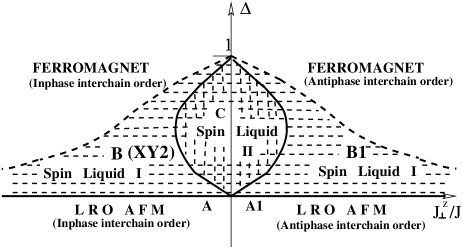
FIG. 2.: The groundstate phase diagram of the two-leg ladder with a longitudinal $J^{z}_{\bot}S^{z}_{j,1}S^{z}_{j,2}$ coupling between legs. For details see text.

The results obtained within the bosonization approach together with the results from the strong coupling expansion allow to draw the following phase diagram of the ladder with a longitudinal interleg coupling $J^{z}_{\bot}$ (see Fig.2). At $\Delta<0$ the phase diagram consists of two gapped phases describing respectively long range ordered Néel antiferromagnetic phases with gapped excitation spectrum and inphase (at $J^{z}_{\bot}<0$) or (antiphase at $J^{z}_{\bot}>0$) ordering of spins within the same rung. The line $\Delta=0$ marks the transition into the Spin Liquid I - phase characterized by a gapless excitation spectrum and power law decay of the spin-spin correlation functions. The critical indices for the decay of the corresponding spin-spin correlations in the Spin Liquid I phase are $\gamma_{i}\simeq 1$. In the case of strong interleg exchange $|J^{z}_{\bot}|\gg J$, further increase of the interleg ferromagnetic exchange $\Delta$ leads to the transition at $\Delta_{c}\simeq J/|J^{z}_{\bot}|$ into the phase with ferromagnetically ordered legs. However, in the weak-coupling case, at $|J^{z}_{\bot}|\ll J$, an increase of the parameter $\Delta$ at given $J^{z}_{\bot}$ leads to the transition into the Spin Liquid II at $\Delta_{c(1)}=|J^{z}_{\bot}|/2J$. The Spin Liquid II phase is characterized by a gapless excitation spectrum and power-law decay of the spin-spin correlation functions with critical indices $\gamma_{i}\simeq 2$. This transition marks the development of the regime dominated by intraleg coupling, whereas the interleg longitudinal exchange plays only a rather moderate role. However, with further increase of the intraleg ferromagnetic exchange, in the vicinity of the ferromagnetic instability line the Spin Liquid II phase becomes unstable and the system reentres into the Spin Liquid I phase. This reentrance effect is connected with a sharp reduction of the bandwidth in the vicinity of the ferromagnetic transition and a subsequent increase of the potential energy of the interleg coupling. Therefore, just before the transition into the ferromagnetically ordered phase, the short range interleg fluctuations get stopped, and as in the case of the strong inrtarung coupling, the Spin Liquid I - phase is unstable toward the transition into the phase with ferromagnetically ordered legs.

However, since the transition into the ferromagnetic phase is a typical finite bandwidth effect, the parameters determined quantitatively within the bosonization (i.e. infinite band) approach strongly depend on the way of regularization of the continuum theory on small distances. Therefore, it is useful to determine the lowest boundary of the ferromagnetic phase on the phase diagram, starting from the ferromagnetically ordered phase and using the standard spin-wave analysis (see appendix). At $|J_{\bot}^{z}|\ll J$ this approach gives $J^{SW}_{FM}=2J\epsilon$. This discrepancy clearly is the result of the linearized expressions used for the parameters $K_{\pm}$, Eq. (27). However, as long as the multiplicative renormalization used here for the parameters $u_{\pm}$ and $K_{\pm}$, Eqs. (26)-(27) remains valid, the scenario discussed above, where the spin liquid I phase is unstable towards the transition into the phase with ferromagnetically ordered legs, remains qualitatively plausible. For a more quantitative description, sufficiently detailed numerical studies of this sector of the phase will be very helpful.

To conclude this subsection we note that the ground state phase diagram of the ferromagnetic ladder system coupled only by the longitudinal part of the spin-spin exchange interaction exhibits a rather rich phase diagram which consist of LRO AFM phases, a spin liquid phase with one gapped and one gapless mode, a spin liquid phase with two gapless modes and a phase with ferromagnetically ordered legs.

B Chains coupled by the transverse part of the ladder exchange

In this subsection we consider the case of two critical Heisenberg chains coupled by a transverse interleg exchange interaction $J^{z}_{\bot}=0$ and $J^{xy}_{\bot}\neq 0$. The particular aspects of this limiting case are the following ones:

• The antisymmetric mode is gapped at arbitrary $J^{xy}_{\bot}\neq 0$.

• The low energy properties of the system are determined by the behavior of the symmetric field.

• The infrared properties of the symmetric field are determined by the subtle coupling between the symmetric and antisymmetric modes.

We start our analysis from the limiting case of weakly anisotropic $XY$ chains, coupled by the weak interleg transverse exchange, assuming $|\Delta|,|{\cal J}^{xy}_{\bot}|/J\ll 1$. At $J^{xy}_{\bot}\neq 0$ the antisymmetric mode is gapped and the dual antisymmetric field is ”pinned” with vacuum expectation value

$$\langle\theta_{-}\rangle=\left\{\begin{array}[]{l}\sqrt{\pi K_{-}/2}\hskip 14.22636pt\textrm{at $J_{\bot}^{xy}>0$}\\ 0\hskip 51.21504pt\textrm{ at $J_{\bot}^{xy}<0$}\end{array}\right.\,.$$ (63)

Behavior of the symmetric field is governed by the SG Hamiltonian (37). The standard RG analysis gives that the symmetric mode is gapped at

$$\Delta<\Delta_{c1}=\frac{\gamma}{4J}\cdot|{\cal J}_{+-}|\,.$$ (64)

Therefore at $\Delta<\Delta_{c1}$ the excitation spectrum of the system is gapped. The dynamical generation of a gap in the symmetric mode leads to condensation of the field $\phi_{+}$ with a vacuum expectation value $\left<\phi_{+}\right>=0$. Since the dual component of the antisymmetric field is ”pinned” with vacuum expectation value given by  (63), the so-called ”disordered” phase [2] is realized in the ground state. At $J_{\bot}^{xy}>0$, spins on the same rung form a singlet and the ground state corresponds to the state with a singlet pair on each rung. There is no correlation between spins along the ladder. In the case of ferromagnetic coupling, at $J_{\bot}^{xy}<0$ spins on the same rung form a state corresponding to the $S^{z}=0$ component of the triplet (an ”asymmetric triplet” pair) and the ground state corresponds to the state with an ”asymmetric triplet” pair on each rung. In analogy to the phases of the $S=1$ chain as discused in [2] we denote this phase as ”anisotropic large D phase”.

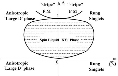
FIG. 3.: The groundstate phase diagram of the two-leg ladder with transverse coupling between legs.

For $\Delta\geq\Delta_{c1}$ the system is in the phase where the symmetric mode is gapless. Since the antisymmetric mode is gapped the alternating part of the spin-spin correlations is exponentially small, while the smooth part shows a power law decay at large distances. In particular, the in-plane correlations are given by

$$K^{xy}_{\alpha\beta}(r)\simeq{\it constant}\cdot\left(-\frac{J^{xy}_{\bot}}{|J^{xy}_{\bot}|}\right)^{\alpha+\beta}r^{-1/4K^{\ast}_{+}}\,$$ (65)

while the longitudinal correlations decay faster

$$K^{zz}_{\alpha\beta}(r)\simeq\frac{K^{\ast}_{+}}{2\pi r^{2}}\,.$$ (66)

As follows from Eq. (65) the line $J_{\bot}^{xy}=0$ marks the transition from a regime with ferromagnetic interleg order into the regime with antiferromagnetic interleg order. In the vicinity of this critical line $J_{\bot}^{xy}=0$ the gap in the antisymmetric mode ($M_{-}$) is tiny, therefore the correlation functions given by Eqs. (65)-(66) are valid only for distances $r\gg L_{c}\sim 1/M_{-}$. However, at distances $r\ll L_{c}$ fluctuations of the antisymmetric mode are strong, and the behavior of correlation functions is the same as in the spin liquid II phase Eqs. (50)-(53). Following Schulz [2] who has discussed a similar phase in the context of the spin $S=1$ chain we denote this phase as a spin liquid XY1 phase.

Let us now discuss the phase diagram of the model in the vicinity of the single chain ferromagnetic instability point $\Delta=1$. As $\Delta\rightarrow 1$, the effective coupling constant behaves as

$$\frac{M^{+}_{eff}}{2\pi u}\simeq\frac{\pi^{2}K{\cal J}_{+-}}{2J}\sim\frac{1}{\epsilon}$$

where $\epsilon=1-\Delta$. A rough estimate of the renormalization of the velocity of the symmetric mode excitations $u_{+}$ and of the spin-liquid parameter $K_{+}$ at $\Delta\simeq 1$, in second order gives

$$u_{+} = u\left(1+\lambda K\left({\cal J}_{+-}/J\right)^{2}\right)\,,$$ (67)

$$K_{+} = K\left(1-\lambda K\left({\cal J}_{+-}/J\right)^{2}\right)\,,$$ (68)

where $\lambda$ is a nonuniversal constant of the order of unity. As follows from Eqs. (67/68) the strong effective transverse coupling reduces the tendency towards ferromagnetic ordering and leads to the transition into the gapped phase at

$${\cal J}_{+-}>{\cal J}_{+-}^{cr}\simeq J(1-\triangle)^{1\over 4}.$$

Equivalently we have

$$\Delta_{c2}\simeq 1-\lambda^{2}({\cal J}_{+-}/J)^{4}.$$

To summarize this subsection we note that the ground state phase diagram of the ferromagnetic ladder system coupled by the transverse part of the spin-spin exchange interaction only also exhibits a rich phase diagram which consist of the ”disordered rung-singlet” and ”anisotropic large D” phases, the easy-plane gapless XY1 phase and the ”stripe” ferromagnetic phases with dominating intraleg ferromagnetic ordering.

C Chains coupled by isotropic interleg exchange

In this subsection we consider the weak-coupling ground state phase diagram of the model  (1) in the case of an isotropic interleg exchange $J^{z}_{\bot}=J^{xy}_{\bot}=:{\cal J}_{\bot}$.

In this case the behavior of the antisymmetric sector is completely similar to the above considered case of the ladder with transverse exchange: the antisymmetric field is gapped and the vacuum expectation value of the dual field $\theta_{-}$, depends on the sign of exchange and is given by Eq. (63) after the substitution ${\cal J}^{xy}_{\bot}\rightarrow{\cal J}_{\bot}$.

The far-infrared properties of the symmetric field are governed by the effective SG Hamiltonian (37) with the bare values of the model parameters given by $K_{+}$ and

$$K_{+} = K\,\left(1-\frac{{\cal J}_{\bot}K}{2\pi u}\right)\,,$$ (69)

$$M^{+}_{eff} = -\frac{1}{\pi u_{+}}{\cal J}_{\bot}\left(1+\delta\right)\,,$$ (70)

(where $\delta$ is a nonuniversal positive number)

The resulting asymmetry of the model is clearly seen:

• at ${\cal J}_{\bot}>0$, the antiferromagnetic interleg exchange reduces $K_{+}$ and increases $M^{+}_{eff}$ and therefore supports the tendencies towards development of a gap in the excitation spectrum

• at ${\cal J}_{\bot}<0$, the ferromagnetic interleg exchange increases $K_{+}$, while with increasing $|{\cal J}_{\bot}|$ the parameter $M^{+}_{eff}\simeq{\cal J}_{\bot}\left(1-\delta\right)\rightarrow 0$ ; therefore we expect an enlargement of the gapless section in this case.

We start our analysis from the limiting case of weakly anisotropic $XY$ chains assuming $|\Delta|,|{\cal J}_{\bot}|/J\ll 1$. At $\Delta=0$ we have $K=1$ and the system shows a gap in the excitation spectrum at ${\cal J}_{\bot}>0$ and is gapless in the case of ferromagnetic interleg exchange ${\cal J}_{\bot}<0$. Therefore at $\Delta=0$, with increasing ferromagnetic interleg exchange (${\cal J}_{\bot}<0,\,|{\cal J}_{\bot}|\rightarrow\infty$) the system continuously evolves into the limit of the $S=1$ $XY$ model, which is known to be gapless [45, 46]. In the case of antiferromagnetic interleg exchange ${\cal J}_{\bot}>0$ the symmetric mode is unstable towards the Kosterlitz-Thouless type transition associated with the dynamical generation of a gap in the excitation spectrum. The weak-coupling RG analysis tells, that at $\Delta\neq 0$ and ${\cal J}_{\bot}>0$ the gapless $XY1$ phase is realized for

$$\Delta>\Delta_{c1}=\frac{{\cal J}_{\bot}}{2J}\left(1+\delta\right)\,,$$ (71)

whereas in the case of ferromagnetic interrung exchange ${\cal J}_{\bot}<0$ it is realized for

$$\Delta>\Delta^{\prime}_{c1}=-{\delta{\cal J}_{\bot}\over 2J}\,.$$

Therefore, from the RG studies we obtain that the gapless $XY1$ phase is stable in the case of ferromagnetic exchange. At ${\cal J}_{\bot}>0$ it is unstable towards the transition into the gapped rung-singlet phase. At ${\cal J}_{\bot}<0$ the gapless $XY1$ phase penetrates into the $\Delta<0$ sector of the phase diagram. However, since $M^{+}_{eff}\rightarrow 0$ with increasing ferromagnetic exchange, at $|{\cal J}_{\bot}|\gg J$ the gapless phase on the antiferromagnetic side ($\Delta<0$) of the phase diagram shrinks up to a narrow stripe which exponentially disappears as $|{\cal J}_{\bot}|/J\to\infty$.

With $\Delta\to 1$ the gapless $XY1$ phase becomes unstable towards transition into the ferromagnetically ordered state. Following the route developed before, we find that at $\Delta=1-\epsilon$ and antiferromagnetic interleg exchange, ${\cal J}_{\bot}>0$, the reentrance of the gapped rung-singlet phase takes place at

$$\Delta_{c2}=1-\frac{{\cal J}_{\bot}}{4J}+{\cal O}\left(\frac{{\cal J}_{\bot}}{4J}\right)^{3/2}\,.$$ (72)

Thus, in agreement with the quasiclassical studies [24], we obtain that two almost ferromagnetically ordered chains coupled by an isotropic interleg exchange are unstable towards formation of the gapped rung-singlet phase at $J_{\bot}>J^{c}_{\bot}>0$, where $J^{c}_{\bot}\rightarrow 0$ as $\Delta\rightarrow 1$. However, in contrast to the quasiclassical case, ${\cal J}^{c2}$ increases linearly with $\epsilon$ in the quantum spin-ladder case.

In the case of ferromagnetic interleg exchange, ${\cal J}_{\bot}<0$, the gapless $XY1$ phase becomes unstable towards the transition into the ferromagnetically ordered phase when $\Delta$ increases towards 1. In this case the spin-wave approach (see appendix) gives that the boundary between the $XY1$ and the ferromagnetic phase is $\Delta=1$.

We summarize our results considering the phase diagram of the ladder with ferromagnetic legs and an isotropic interleg exchange in Fig. 4.

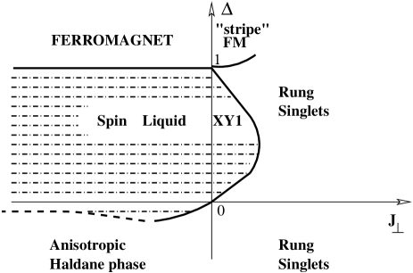
FIG. 4.: The ground state phase diagram of the two-leg ladder with an isotropic interleg coupling.

IV Conclusions

We have studied the ground state phase diagram of the $S=1/2$ ladder with ferromagnetically interacting legs using the continuum limit bosonization approach. The phase diagrams for the extreme anisotropic interchain coupling cases (Ising and $XY$ interleg exchange) as well as for the $SU(2)$ symmetric case were obtained. These phase diagrams exhibit a number of interesting phases, gapped as well as gapless; some of these are familiar from well known 1D models (rung singlet phase, anisotropic Haldane phase, ferromagnetic and large $D$ phase), in addition we describe here for the first time less conventional phases for ladders: the spin liquid phases with (i) one gapless and one gapped mode (including the known $XY1$ and $XY2$ phases) and (ii) two gapless modes. We have shown moreover that the gapped rung singlet phase found semiclassically to appear for an arbitrarily small isotropic antiferromagnetic interaction between ferromagnetic legs [24] continues to exist for $S=1/2$ ladders and $xy-$like interactions and actually extends to small values of $\Delta$.

The neighborhood of the single chain ferromagnetic instability point turned out to be of particular interest. We investigated the behavior of the system in this regime using the multiplicative regularization scheme. This scheme allows to extend the bosonization formalism to the limit when the bandwidth of the single chain excitations collapses and leads to the result that upon increasing the strength of ferromagnetism $\Delta$ at any moderate fixed interleg interaction a sequence of two phase transitions occurs before the system enters the final ferromagnetically ordered phase.

Preliminary investigations show that the system considered here displays additional interesting aspects when an external magnetic field (both longitudinal and transverse) is applied. These investigations will be reported in a subsequent publication.

V Acknowledgments

It is a pleasure to thank A.K. Kolezhuk for helpful discussions. TV is grateful to A.A. Nersesyan for various enlightening discussions. GIJ thanks W. Brenig and A. Honecker for interesting discussion. He also acknowledges support by the SCOPES grant N 7GEPJ62379. This work is supported by the DFG-Graduiertenkolleg No. 282, ”Quantum Field Theory Methods in Particle Physics, Gravitational Physics, and Statistical Physics”.

A Ferromagnetic instability

In this appendix we consider ferromagnetic interleg coupling, assuming $J^{xy}_{\bot},J^{z}_{\bot}<0$, and use the spin wave approach to determine the critical line corresponding to the ferromagnetic instability in our system. For this purpose we start from the region of the phase diagram where we can safely assume that the ground state is the fully polarized ferromagnetic state (that is $\Delta\gg 1$ and $J_{\bot}<0$). We identify the transition line from the fully polarized ground state to some other state as the line of instability in the spin wave excitation spectrum.

Let us denote the eigenstate of the Hamiltonian (1) corresponding to the fully polarized (along the $Z$ axis) ferromagnetic state by $\left|0\right>$. Then

$$S_{j,\alpha}^{+}\left|0\right>=0,\qquad\mbox{for arbitrary j and}\quad\alpha.$$

It is straightforward to obtain that $\hat{H}\left|0\right>=E_{0}\left|0\right>$ where

$$E_{0}=-{N\over 4}\left(\left|J^{z}_{\bot}\right|+2J\Delta\right).$$

To construct the lowest excitations in the ferromagnetic phase we act on the ground state configuration by the spin lowering operator $S_{n,\alpha}^{-}$. Let us denote by $\left|1\right>_{n}$ ($\left|2\right>_{n}$) the state obtained by action of the spin lowering operator on the $n^{\rm th}$ site of leg 1 (leg 2):

$$\left|1\right>_{n}\equiv S_{n,1}^{-}\left|0\right>,\quad\left|2\right>_{n}\equiv S_{n,2}^{-}\left|0\right>\,.$$

It is straightforward to solve the coupled system of equations of motion in the subspace $S^{z}_{\rm tot}=N-1$ and to obtain the following two sets of excitation frequencies:

$$\omega^{-}(q) = -J\cos q+J\Delta-{1\over 2}\left(J^{z}_{\bot}-J^{xy}_{\bot}\right)$$ (A1)

$$\omega^{+}(q) = -J\cos q+J\Delta-{1\over 2}\left(J^{z}_{\bot}+J^{xy}_{\bot}\right)\,.$$ (A2)

For ferromagnetic interleg exchange ($J^{z}_{\bot},J^{xy}_{\bot}<0$) we have

$$\omega^{-}(q)<\omega^{+}(q)$$

and from the instability condition $\omega^{-}(q=0)=0$ we obtain

$$\Delta=1+\frac{1}{2J}\left(J^{z}_{\bot}-J^{xy}_{\bot}\right)\,.$$ (A3)

In the particular limit of noninteracting chains $(J^{z}_{\bot}=J^{xy}_{\bot}=0)$ as well as in the limiting case of the rotationally invariant interleg coupling $(J^{z}_{\bot}=J^{xy}_{\bot})$ the critical line corresponding to the instability of the ferromagnetic phase is given by the condition

$$\Delta=1\,.$$ (A4)

REFERENCES

- [1] For a review see E. Dagotto, Rep. Prog. Phys. 62, 1525 (1999); E. Dagotto and T.M. Rice, Science 271, 618 (1996).
- [2] H.J. Schulz, Phys. Rev. B 34, 6372, (1986).
- [3] I. Affleck, J. Phys. Condens. Matter 1, 3047 (1991).
- [4] D.G. Shelton, A.A. Nersesyan and A.M. Tsvelik, Phys. Rev. B 53, 8521 (1996).
- [5] A.K. Kolezhuk and H.-J. Mikeska, Phys. Rev. B 56, R11380 (1997).
- [6] F.D.M. Haldane, Phys. Rev. Lett. 50, 1153 (1983); Phys. Lett. A 93, 464 (1983).
- [7] E. Dagotto and A. Moreo, Phys. Rev. B 38, 5087 (1988); Phys. Rev. B 44, 5396(E) (1991).
- [8] K. Hida, J. Phys. Soc. Jpn. 60, 1347 (1991).
- [9] S.P. Strong and A.J. Millis, Phys. Rev. Lett. 69, 2419 (1992).
- [10] E. Dagotto, J. Riera and D. Scalapino, Phys. Rev. B 45, 5744 (1992).
- [11] S. Takada and H. Watanabe, J. Phys. Soc. Jpn. 61, 39 (1992).
- [12] H. Watanabe, K. Nomura and S. Takada, J. Phys. Soc. Jpn. 62, 2845 (1993).
- [13] T. Barnes, E. Dagotto, J. Riera and E.S. Swanson, Phys. Rev. B 47, 3196 (1993).
- [14] T.M. Rice, S. Gopalan and M. Sigrist, Europhys. Lett. 23, 445 (1993).
- [15] S. Gopalan, T.M. Rice and M. Sigrist, Phys. Rev. B 49, 8901 (1994); M. Sigrist, T.M. Rice and F.C. Zhang, ibid. 49, 12058 (1994).
- [16] R.M. Noack, S.R. White, and D.J. Scalapino, Phys. Rev. Lett. 73, 882 (1994).
- [17] S.R. White, R.M. Noack and D.J. Scalapino, Phys. Rev. Lett. 73, 886 (1994).
- [18] D. Poilblanc, H. Tsunetsugu and T.M. Rice, Phys. Rev. B 50, 6511 (1994).
- [19] T. Barnes and J. Riera, Phys. Rev. B 50, 6817 (1994).
- [20] S.P. Strong and A.J. Millis, Phys. Rev. B 50, 9911 (1994).
- [21] M. Totsuka and M. Suzuki, J. Phys. Condens. Matter 7, 6079 (1995).
- [22] S.R. White, Phys. Rev. B. 53, 52, (1996).
- [23] A.K. Kolezhuk and H.-J. Mikeska, Int. J. Mod. Phys. B 12, 2325 (1998).
- [24] A.K. Kolezhuk and H.-J. Mikeska, Phys. Rev. B 53, R8848 (1996).
- [25] M. Roji and S. Miyashita, J. Phys. Soc. Jap. 65, 883 (1996).
- [26] A.A. Nersesyan and A.M. Tsvelik, Phys. Rev. Lett. 78, 3939 (1997).
- [27] Ö. Legeza and J. Sólyom, Phys. Rev. B 56, 14449 (1997).
- [28] A.A. Nersesyan, A.O. Gogolin and F.H.L. Essler, Phys. Rev. Lett. 81, 910 (1998).
- [29] D.C. Cabra, A. Honecker and P. Pujol, Phys. Rev. B 58, 6241 (1998).
- [30] T. Giamarchi and A.M. Tsvelik, Phys. Rev. B 59, 11398 (1999).
- [31] E.H. Kim and J. Sólyom Phys. Rev. B 60, 15230 (1999).
- [32] D. Allen, F.H.L. Essler and A.A. Nersesyan, Phys. Rev. B 61, 8871 (2000).
- [33] E.H. Kim, G. Fáth, J. Sólyom and D.J. Scalapino, Phys. Rev. B 62, 14965 (2000).
- [34] G. Fáth, Ö. Ligeza and J. Sólyom, Phys. Rev. B 63, 134403 (2001).
- [35] M. Müller, T. Vekua and H.-J. Mikeska, preprint cond-mat/0206081.
- [36] A. Luther and I. Peschel, Phys. Rev. B 12, 3908 (1975).
- [37] I. Affleck, in Champs, Cordes et Phénomènes Critiques/ Fields, strings and critical phenomena, Eds. E. Brézin and J. Zinn-Justin, Elsevier, Amsterdam, (1990).
- [38] R. Shankar, Int. J. Mod. Phys. B 4, 2371 (1990).
- [39] A.O. Gogolin, A.A. Nersesyan and A.M. Tsvelik, Bosonization and Strongly Correlated Systems, Cambridge University Press (1999).
- [40] S. Lukyanov, V. Terras, preprint hep-th/0206093.
- [41] T. Hikihara and A. Furusaki, Phys. Rev. B 58, R583 (1998).
- [42] J.M. Kosterlitz and D.J. Thouless, J. Phys. C 11, 1583 (1973).
- [43] P. Wiegmann, J. Phys. C 11, 1583 (1978).
- [44] K.A. Muttalib and V.J. Emery, Phys. Rev. Lett. 57, 1370 (1986).
- [45] K. Kubo, Phys. Rev. B 46, 866 (1992).
- [46] A. Kitazawa, K. Nomura and K. Okamoto, Phys. Rev. Lett. 76, 4038 (1996).