Phase Transition in the ABC model

Abstract

Recent studies have shown that one-dimensional driven systems can exhibit phase separation even if the dynamics is governed by local rules. The ABC model, which comprises three particle species that diffuse asymmetrically around a ring, shows anomalous coarsening into a phase separated steady state. In the limiting case in which the dynamics is symmetric and the parameter $q$ describing the asymmetry tends to one, no phase separation occurs and the steady state of the system is disordered. In the present work we consider the weak asymmetry regime $q=\exp{(-\beta/N)}$ where $N$ is the system size and study how the disordered state is approached. In the case of equal densities, we find that the system exhibits a second order phase transition at some nonzero $\beta_{c}$. The value of $\beta_{c}=2\pi\sqrt{3}$ and the optimal profiles can be obtained by writing the exact large deviation functional. For nonequal densities, we write down mean field equations and analyze some of their predictions.

I Introduction

Nonequilibrium steady states, wherein the properties of a system are stationary but the steady state probabilities are not described by Boltzmann weights with respect to a local energy function, may exhibit a number of interesting phenomena absent from equilibrium systems: for example, driven diffusive systems KLS have generically long-range correlations; phase transitions may also occur in one-dimensional non-equilibrium steady states although they are of course precluded from one-dimensional equilibrium systems with short-range interactions.

Examples of nonequilibrium phase transitions include the absorbing state phase transitions Haye and boundary induced phase transitions in driven systems wherein a conserved current is driven through a finite open system krug ; DDM ; DEHP ; SD ; EFGM . Bulk (i.e. not boundary-driven) phase transitions may arise in systems with no absorbing states like conserving driven systems through the introduction of several species of particles DJLS ; Mallick ; Evans96 ; AHR ; KLMT ; EKLM .

Phase separation has been exhibited in several one dimensional driven systems EKKM ; LBR ; AHR consisting of several species of particles with nearest neighbour exchanges occurring with prescribed rates. Models in this class are the ABC model EKKM , the AHR model AHR ; RSS ; KLMT – which both contain three species of particles – and the LR model LBR which consists of two sublattices with two species each. The phase separation in these models has the striking feature of the domains of each species being pure. That is, far away from the domain walls, there is zero probability of finding a particle of one species in a domain of a different species. This is referred to as strong phase separation.

An understanding of this phenomenon has emerged through the exact solution of the steady state in some special cases of the ABCEKKM and the LR modelLBR . Even though the dynamics is strictly local, in these special cases it has been shown that the steady state obeys detailed balance with respect to a long-range energy function. The long-range interaction leads to superextensivity of this energy function i.e. the energy of most microscopic configurations scales quadratically with system size $N$ so that the contribution of the entropy becomes negligible. Almost all configurations are therefore suppressed and only strongly phase separated configurations contribute. Although generally in the ABC and the LR models for non-equal numbers of particles detailed balance does not hold and one does not have an energy function, the same strong phase separation is observed in simulations EKKM .

In the ABC model there is a parameter $q$ that governs the local dynamics. It describes the asymmetry in the rates of nearest neighbour particle exchanges (see section II). If $q<1$ is held fixed then one always has strong phase separation in the thermodynamic limit ($N\to\infty$). However for $q=1$, in which case the particles exchange symmetrically, the system is in a homogeneous disordered state where all configurations are equally probable. In the present work we investigate the ABC model in what we shall refer to as the weak asymmetry regime. That is, we introduce a system size dependence into $q$ so that an extensive energy is recovered (when an energy function indeed exists). It turns out that the appropriate choice of $q$ is

$$q=\exp{\left(-\frac{\beta}{N}\right)}\;.$$ (1)

Thus $\beta$ is now the control parameter and plays the role of an inverse temperature i.e. $\beta=1/T$. In this regime an interesting question is as to how the transition from the strongly phase separated state to the disordered state occurs as $T$ is varied. Since the energy function is long range it is possible to have a phase transition at a well defined temperature $T_{c}=\beta_{c}^{-1}$ even though the system is one dimensional (phase transitions in fact do occur in one-dimensional systems with algebraically decaying interaction FMN or in the Bernasconi model Bernasconi which is an Ising spin model with energy function given by long-range, four spin interactions MPR ).

In the present paper, we first summarize in section II some known facts about the ABC model. In section III, we present our results of Monte Carlo simulations done in the weak asymmetry regime for an equal number of particles of each species. These simulations indicate that there is a critical value $\beta_{c}={1\over T_{c}}\simeq 11$. In Section IV we derive the exact free energy functional for an arbitrary density profile from the expression for the weights in the steady state in the case of equal particle numbers. By minimizing this functional we obtain the exact value of $\beta_{c}=2\pi\sqrt{3}\simeq 10.88\dots$ and the shape of the density profiles in the neighbourhood of the transition. In section V, we investigate the case of arbitrary global densities within a mean field approximation. We observe that this approximation turns out to be exact in the case of equal numbers of particles.

II The ABC model

The ABC model is defined on a 1d ring with $N$ lattice sites. Each site is occupied by one of three types of particles denoted as $A$, $B$ or $C$. They exhibit hard-core interaction, i.e. only one particle per site is allowed. Neighboring sites on the ring are exchanged according to the following rates:

$$AB {{q\atop\longrightarrow}\atop{\longleftarrow\atop 1}} BA$$ (2)

$$BC {{q\atop\longrightarrow}\atop{\longleftarrow\atop 1}} CB$$ (3)

$$CA {{q\atop\longrightarrow}\atop{\longleftarrow\atop 1}} AC$$ (4)

Thus for $q\neq 1$ the particles diffuse asymmetrically around the ring and in the case $q=1$ they diffuse symmetrically. Note that periodic boundary conditions are implied and the dynamics conserves the number of particles.

This model has been extensively studied in EKKM by analytical and numerical means. Let us summarise in this section the main results. Starting from an initially random configuration, the system coarsens into a strongly phase separated state for any $q\neq 1$. Thus the steady state exhibits long-range order, even though the dynamics is strictly local. We will restrict our discussion of $q\neq 1$ to the case $q<1$ for simplicity. (The case $q>1$ can be obtained by the transformation $q\to 1/q$ together with the exchange of $A$ and $B$ particles). For $q=1$ particles of all species have equivalent dynamics which results in a steady state in which all configurations have equal weight and the steady state of the system is disordered.

To understand the coarsening dynamics for $q<1$, note that domain walls of the type $BA$, $CB$ and $AC$ are unstable to interchanges leading to $AB$, $BC$ and $CA$ respectively. Therefore $A$ particles are driven to the left in a $B$ domain and to the right in a $C$ domain (particles $B$ and $C$ are also driven in other species domains). Thus the system arrives at a metastable configuration of the form $A\dots AB\dots BC\dots CA\dots AB\dots BC\dots CA\dots$ and a slow coarsening process, involving the elimination of the smallest domains, ensues. For example, the time it takes an $A$ particle to traverse a $B$ domain of length $l$ is of order $q^{l}$. Thus the elimination of domains of size $l$ occurs at a rate of order $q^{-l}$ which results in the typical domain size growing as $l\sim\ln t$. This growth law which is slower than any power of $t$ is referred to as anomalous coarseningEvans . Ultimately the coarsening process results in a strongly phase separated state comprising three pure domains.

The general steady state is not, as yet, known. In the special case of equal particle numbers $N_{A}=N_{B}=N_{C}=N/3$, however, one can show that the steady state obeys detailed balance with respect to a long-range energy function $\mathcal{H}$. A configuration of the system is specified by the set of indicator variables $\{X_{i}\}=\{A_{i},B_{i},C_{i}\}$ which take values 1 or 0 according to whether site $i$ is occupied by the relevant particle. For example $A_{i}=1$ if site $i$ is occupied by an $A$ particle. Clearly, these variables satisfy $A_{i}+B_{i}+C_{i}=1$. With these indicator variables the energy function may be written as:

$$\mathcal{H}(\{X_{i}\})={1\over N}\sum_{i=1}^{N}\sum_{k=1}^{N-1}k\left(B_{i}C_{i+k}+C_{i}A_{i+k}+A_{i}B_{i+k}\right)$$ (5)

and the steady state weights of the system are given by

$$P(\{X_{i}\})=Z_{N}^{-1}q^{\mathcal{H}(\{X_{i}\})}$$ (6)

where $Z_{N}=\sum q^{\mathcal{H}(\{X_{i}\})}$ denotes the partition function. Note that the energy given in EKKM differs by a constant from (5).

In (5) the interaction between sites $i$ and $i+k$ are both long-range and asymmetric and the energy function is superextensive and scales quadratically with system size $N$.

The width of the domain walls in the phase separated state is of order $1/|\ln{q}|$ EKKM . So for $q\to 1$ the size of the domain walls diverges and the system will be in a homogeneous disordered state. Moreover we expect an interesting regime to occur when the width of the domain walls is of the order of the domain lengths $N/3$ i.e.

$$\frac{1}{|\ln{q}|}\sim O(N)$$ (7)

This yields the weakly asymmetric regime stated in the introduction (1) where the control parameter is now $T=1/\beta$. The steady state weight (5,6) also confirms that (1) is the natural choice of scaling variable since under this scaling (6) becomes

$$P_{N}(\{X_{i}\})=Z_{N}^{-1}\exp{\left(-\beta E_{N}(\{X_{i}\})\right)}$$ (8)

where $Z_{N}$ is a normalization constant (the partition function) and the extensive rescaled energy $E_{N}(\{X_{i}\})$ is defined as

$$E_{N}(\{X_{i}\})=\mathcal{H}(\{X_{i}\})/N\;\quad.$$ (9)

III Monte Carlo Simulations

We have measured by Monte-Carlo simulations the number of nearest neighbour pairs of sites occupied by the same species of particles in the steady state. We shall refer to these as nearest neighbour (nn) matching pairs. For a completely disordered system (i.e. for $\beta=0$) the probability of finding a nn matching pair is $1/3$ for large $N$. As $\beta$ increases, one expects this number to increase and to be equal to 1 as $\beta\to\infty$ (i.e. as one reaches the strongly separated regime).

In figure 1, we show the results of our simulations for $m_{N}$ defined as

$$m_{N} = \frac{\mbox{number of nn matching pairs}}{\mbox{system size}}-\frac{1}{3}$$ (10)

$$= \frac{1}{N}\sum_{i=1}^{N}\left[\;A_{i}A_{i+1}+B_{i}B_{i+1}+C_{i}C_{i+1}\right]-\frac{1}{3}\;,$$ (11)

with the occupation variable $X_{i}=A_{i},B_{i},C_{i}$ defined as in (5). Note that because of the periodic boundary conditions, site $N+1$ is identified with site $1$. We see that as $N$ increases, $m_{N}$ seems to be closer and closer to zero as $\beta<11$ whereas it seems to have a well-defined limit $m$ which depends on $\beta$ for $\beta>11$

$$m=\lim_{N\to\infty}m_{N}\;.$$ (12)

Note that $m$ only contains nearest neighbour correlations as opposed to e.g. the measure of order used in EKKM which contains long range terms. Also one could consider the lowest Fourier mode of the density profile (see section IV).

Figure 1: Parameter $m$ defined by (11) for system sizes $N=30$ to $240$

For $T<T_{c}$ we expect $0<m<2/3$ with $m$ approaching $2/3$ in the limit $T\to 0$. This behaviour can be seen in Fig. 1. For $1/T\approx 11$ a crossover from an ordered to a disordered state appears which becomes sharper with increasing system size. In Fig. 2 we plot the specific heat defined as $C_{N}=\partial\overline{E_{N}}/\partial T$. One sees strong finite size effects at $\beta=1/T\approx 11$. Moreover, the curves suggest that a discontinuity emerges in the infinite system limit which would be consistent with a second-order phase transition.

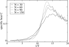
Figure 2: Specific heat for system sizes $N=30,60,90,150$

To determine the critical temperature of the system, we have performed a standard finite size scaling analysis Binder based on the distribution of the parameter $m_{N}$ defined as in (11). Such an analysis has already proved to be effective in the study of non-equilibrium steady states OLE ; TP . We performed Monte Carlo simulations of the model for system sizes $N=30$ to $210$ over $10^{9}$ sweeps in the steady state for each set of parameters. To determine the critical temperature $T_{c}$ we measured the ratio between two moments of the parameter $m_{N}$

$$U_{N} = 1-\frac{\langle m_{N}^{4}\rangle}{3\langle m_{N}^{2}\rangle^{2}}\quad.$$ (13)

(In fact, since one does not have to distinguish between positive and negative values of the parameter $m$, the ratio $\langle m^{2}\rangle/\langle m\rangle^{2}$ could as well be used to determine the critical temperature.)

At the critical temperature $T_{c}$, $U_{N}$ has a universal value $U^{*}$. Thus on measuring $U_{N}$ for various system sizes as a function of $T$, $U^{*}$ is the common intersection point of the curves and identifies $T_{c}$. Our results shown in Fig. 3 indicate $\beta_{c}=1/T_{c}\simeq 10.95$.

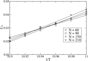
Figure 3: Critical temperature $T_{c}$ as intersection point $U^{*}$ of the fourth-order cumulant of the order parameter $U_{N}$ (the straight lines are linear fits to the data)

IV Large deviation functional for equal densities and the exact transition temperature

In this section we consider only the case of equal numbers of each species

$$N_{A}=N_{B}=N_{C}={N\over 3}$$ (14)

where there exists an energy function given by (5,9)

$$E_{N}(\{X_{i}\})=\frac{1}{N^{2}}\sum_{i=1}^{N-1}\sum_{k=1}^{N-1}k\left(B_{i}C_{i+k}+C_{i}A_{i+k}+A_{i}B_{i+k}\right)$$ (15)

with the occupation variables $\{X_{i}\}=\{A_{i},B_{i},C_{i}\}$ defined as in (5). The steady state probabilities of the system are given by (8).

We pass to the continuum limit where $\rho_{A}(x),\rho_{B}(x),\rho_{C}(x)$ are the density profiles of $A,B,C$ particles respectively at position $x=i/N$. Then the free energy functional DLS1 ; DLS2 (or large deviation functional) ${\cal F}[\rho_{A}(x),\rho_{B}(x),\rho_{C}(x)]$ which gives the probability of any density profile through

$$P[\rho_{A}(x),\rho_{B}(x),\rho_{C}(x)]=\exp\{-N{\cal F}[\rho_{A}(x),\rho_{B}(x),\rho_{C}(x)]\}$$ (16)

can be written in terms of the density profiles as

$${\cal F}[\rho_{A}(x),\rho_{B}(x),\rho_{C}(x)]=K$$ (17)

$$+ \int_{0}^{1}dx\left[\rho_{A}(x)\ln\rho_{A}(x)+\rho_{B}(x)\ln\rho_{B}(x)+\rho_{C}(x)\ln\rho_{C}(x)\right]$$

$$+ \beta\int_{0}^{1}dx\int_{0}^{1}dz\left[\rho_{B}(x)\rho_{C}(x+z)+\rho_{C}(x)\rho_{A}(x+z)+\rho_{A}(x)\rho_{B}(x+z)\right]z$$

where $\rho_{A},\rho_{B},\rho_{C}$ are periodic functions of period $1$ and $K$ is a normalization constant such that the minimum of ${\cal F}$ over all profiles vanishes. The second term on the right hand side of (17) represents the entropy of the given profiles while the term proportional to $\beta$ is the continuum form of the energy (15).

It is easy to derive an expression for the optimal profile for $\rho_{A}(x)$ by finding the extremum of (17) with respect to $\rho_{A}(x)$ subject to the constraint that

$$\int\rho_{A}(x)dx=1/3\;.$$

One obtains

$$\rho_{A}(x)=\mbox{Constant}\times\exp\left(-\beta\int_{0}^{1}[\rho_{B}(x+z)+\rho_{C}(x-z)]zdz\right)\;.$$ (18)

which implies that

$$\frac{d\rho_{A}(x)}{dx}=-\beta\rho_{A}(x)\left(\rho_{B}(x)-\rho_{C}(x)\right)\;.$$ (19)

Similar equations hold for $\rho_{B}(x)$ and $\rho_{C}(x)$ and using $\rho_{C}(x)=1-\rho_{A}(x)-\rho_{B}(x)$ one obtains the coupled equations

$$\frac{d\rho_{A}(x)}{dx} = -\beta\rho_{A}(x)\left(\rho_{A}(x)+2\rho_{B}(x)-1\right)$$ (20)

$$\frac{d\rho_{B}(x)}{dx} = -\beta\rho_{B}(x)\left(1-2\rho_{A}(x)-\rho_{B}(x)\right)\;.$$ (21)

Clearly one solution of (20,21) is $\rho_{A}(x)=\rho_{B}(x)=1/3$ which corresponds to the disordered phase, but this extremum is the minimum only in the disordered phase. To test when an ordered solution emerges we define the Fourier series of arbitrary profiles as

$$\rho_{A}(x) = 1/3+\sum_{n=1}^{\infty}\left[a_{n}\exp(i2\pi nx)+a_{-n}\exp(-i2\pi nx)\right]$$ (22)

$$\rho_{B}(x) = 1/3+\sum_{n=1}^{\infty}\left[b_{n}\exp(i2\pi nx)+b_{-n}\exp(-i2\pi nx)\right]$$ (23)

$$\rho_{C}(x) = 1/3+\sum_{n=1}^{\infty}\left[c_{n}\exp(i2\pi nx)+c_{-n}\exp(-i2\pi nx)\right]$$ (24)

We insert these into (20,21) and, anticipating a continuous phase transition, expand to first order in $a_{n},b_{n}$. We look for values of $\beta$ for which a solution for nonzero $a_{n}$, $b_{n}$, $c_{n}$ is present and therefore the uniform solution could be unstable. One finds that the uniform solution becomes unstable to the $n$th mode for $\beta^{2}/3=(2\pi n)^{2}$ so that the first instability occurs at $\beta_{c}$ given by

$$\beta_{c}=2\pi\sqrt{3}=10.882796...\;.$$ (25)

Near $\beta_{c}$ equations (20,21) can be solved perturbatively in

$$\epsilon=\frac{\beta-\beta_{c}}{\beta_{c}}\;.$$ (26)

One finds to leading order

$$\rho_{A}(x)=\rho_{B}\left(x+{1\over 3}\right)=\rho_{C}\left(x+{2\over 3}\right)=$$ (27)

$$\frac{1}{3}+\left(\epsilon\over 6\right)^{1/2}2\cos(2\pi(x-x_{0}))+\left(\epsilon\over 6\right)2\cos(4\pi(x-x_{0}))+O(\epsilon^{3/2})$$

where $x_{0}$ can be arbitrary (as an optimal profile remains optimal when it is translated). Also, choosing $x_{0}=0$, one can show that $a_{n}=a_{-n}$ and $a_{3m}=0\;$ for $|m|=0,1\ldots$ to all orders in $\epsilon$ and that to leading order in $\epsilon$

$$a_{1}\sim\left(\frac{\epsilon}{6}\right)^{1/2}\;,\quad a_{2}\sim\left(\frac{\epsilon}{6}\right)\;,\quad a_{4}\sim-\left(\frac{\epsilon}{6}\right)^{2}\;,\quad a_{5}\sim-\left(\frac{\epsilon}{6}\right)^{5/2}\ldots$$ (28)

The parameter $m$ defined as in (12,11) becomes in the continuum limit

$$m=\int_{0}^{1}[\rho^{2}_{A}+\rho^{2}_{B}+\rho^{2}_{C}]dx\ -\ \frac{1}{3}\;.$$ (29)

and from (27) one obtains

$$m\sim\frac{\beta-\beta_{c}}{\beta_{c}}\;.$$ (30)

Thus the parameter $m$ as defined in (12,11) vanishes linearly at the transition. An alternative, and probably more standard, choice for the order parameter could be the amplitude $a_{1}$ of the fundamental mode KSZ and this would lead to an exponent $1/2$.

We now turn to the calculation of the energy. For arbitrary density profiles the energetic contribution to the free energy (15) may be written in terms of the Fourier coeffcients as

$$E=\frac{1}{6}-\sum_{n\neq 0}\frac{a_{n}b_{-n}+b_{n}c_{-n}+c_{n}a_{-n}}{2\pi in}$$ (31)

For profiles $\rho_{B}(x)=\rho_{A}(x-1/3)$, $\rho_{C}(x)=\rho_{A}(x-2/3)$ this energy becomes

$$E=\frac{1}{6}-3\sum_{n=1}^{\infty}\frac{a_{n}a_{-n}}{n\pi}\sin(2\pi n/3)\;.$$ (32)

Thus, using (28), near $\beta_{c}$ we have $E\simeq 1/6-3\epsilon/2\beta_{c}$ and the heat capacity $-\beta^{2}\partial E/\partial\beta$ has a discontinuity of 3/2 at $\beta_{c}$, consistent with the data of figure 2.

This equal density case is similar to some special cases found in a recent study of the dynamical winding of random walksFF for which the fact that the dynamics satisfies detailed balance allows one to write equations for the density profiles of the type (20) and to locate the exact transition point.

V Non-equal Densities and mean-field theory

We now turn to the case of non-equal densities of particles. A direct consequence of the stochastic dynamical rules (4) is that

$${d\langle A_{i}\rangle\over dt}=q\langle A_{i-1}B_{i}\rangle+q\langle C_{i}A_{i+1}\rangle+\langle B_{i}A_{i+1}\rangle+\langle A_{i-1}C_{i}\rangle$$

$$-q\langle A_{i}B_{i+1}\rangle-q\langle C_{i-1}A_{i}\rangle-\langle B_{i-1}A_{i}\rangle-\langle A_{i}C_{i+1}\rangle$$ (33)

and similar equations hold for ${d\langle B_{i}\rangle\over dt}$ and ${d\langle C_{i}\rangle\over dt}$. We do not know how to solve these exact equations, in particular because they require the knowledge of two point functions. One can, however, write down mean-field equations DDM , by making an approximation which neglects correlations (i.e. where one replaces correlation functions such as $\langle A_{i-1}B_{i}\rangle$ by $\langle A_{i-1}\rangle\langle B_{i}\rangle$)

$${d\langle A_{i}\rangle\over dt}=q\langle A_{i-1}\rangle\langle B_{i}\rangle+q\langle C_{i}\rangle\langle A_{i+1}\rangle+\langle B_{i}\rangle\langle A_{i+1}\rangle+\langle A_{i-1}\rangle\langle C_{i}\rangle$$

$$-q\langle A_{i}\rangle\langle B_{i+1}\rangle-q\langle C_{i-1}\rangle\langle A_{i}\rangle-\langle B_{i-1}\rangle\langle A_{i}\rangle-\langle A_{i}\rangle\langle C_{i+1}\rangle$$ (34)

Assuming that the profiles vary slowly with $i$, we write $\rho_{A}(x)=\langle A_{i}\rangle$ and

$$\langle A_{i\pm 1}\rangle=\rho_{A}(x)\pm\frac{1}{N}\frac{\partial\rho_{A}(x)}{\partial x}+\frac{1}{2N^{2}}\frac{\partial^{2}\rho_{A}(x)}{\partial x^{2}}+\ldots$$ (35)

then keeping leading order terms in $1/N$ and defining $\tau=N^{2}t$ in (36) yields

$$\frac{\partial\rho_{A}}{\partial\tau}=\beta\frac{\partial}{\partial x}\left[\rho_{A}(\rho_{B}-\rho_{C})\right]+\frac{\partial^{2}\rho_{A}}{\partial x^{2}}$$

$$\frac{\partial\rho_{B}}{\partial\tau}=\beta\frac{\partial}{\partial x}\left[\rho_{B}(\rho_{C}-\rho_{A})\right]+\frac{\partial^{2}\rho_{B}}{\partial x^{2}}$$ (36)

$$\frac{\partial\rho_{C}}{\partial\tau}=\beta\frac{\partial}{\partial x}\left[\rho_{C}(\rho_{A}-\rho_{B})\right]+\frac{\partial^{2}\rho_{C}}{\partial x^{2}}$$

One can linearize these equations around constant density profiles

$$\rho_{A}(x)=r_{A}+\Delta\rho_{A}(x)\;,\quad\rho_{B}(x)=r_{B}+\Delta\rho_{B}(x)\;,\quad\rho_{C}(x)=r_{C}+\Delta\rho_{C}(x)$$ (37)

where $\Delta\rho_{A}(x),\Delta\rho_{B}(x),\Delta\rho_{C}(x)$ represent small departures from constant profiles at densities $r_{A}=N_{A}/N,r_{B}=N_{B}/N,r_{C}=N_{C}/N$ ($r_{A},r_{B},r_{C}$ are the global densities of the three species and of course they satisfy $r_{A}+r_{B}+r_{C}=1$). Then one finds that these small departures are damped when $\beta<\beta_{c}^{\rm mf}$ given by

$$\beta_{c}^{\rm mf}=\frac{2\pi}{\left(2r_{A}r_{B}+2r_{A}r_{C}+2r_{B}r_{C}-r_{A}^{2}-r_{B}^{2}-r_{C}^{2}\right)^{1/2}}=\frac{2\pi}{\left[1-2(r_{A}^{2}+r_{B}^{2}+r_{C}^{2})\right]^{1/2}}$$ (38)

We see that in the equal density case ($r_{A}=r_{B}=r_{C}=1/3$), the mean field value of $\beta_{c}$ coincides with the exact value (25). Moreover one finds that the solutions of the exact equations for the optimal profile (19) are steady state solutions of the mean field equations (36) (as they make the l.h.s. of these equations vanish). So, at least for the equal time properties, in this equal density case, $\beta_{c}$ and the profiles predicted by the mean field theory are exact.

Near $\beta_{c}$, one can perturbatively find stationary non-moving profiles. The first Fourier mode of these profiles is given by

$$\Delta\rho_{A}(x) \simeq \psi(\epsilon)\left[\sqrt{r_{A}}\ e^{2i\pi(x-x_{0})}+c.c.\right]$$ (39)

$$\Delta\rho_{B}(x) \simeq \psi(\epsilon)\left[{r_{C}-r_{A}-r_{B}-i\sqrt{1-2(r_{A}^{2}+r_{B}^{2}+r_{C}^{2})}\over 2\sqrt{r_{A}}}e^{2i\pi(x-x_{0})}+c.c.\right]$$ (40)

$$\Delta\rho_{C}(x) \simeq \psi(\epsilon)\left[{r_{B}-r_{A}-r_{C}+i\sqrt{1-2(r_{A}^{2}+r_{B}^{2}+r_{C}^{2})}\over 2\sqrt{r_{A}}}e^{2i\pi(x-x_{0})}+c.c.\right]$$ (41)

where $\epsilon$ is defined as in (26) and

$$\psi(\epsilon)={1-2(r_{A}^{2}+r_{B}^{2}+r_{C}^{2})\over\sqrt{2(r_{A}^{2}+r_{B}^{2}+r_{C}^{2})-4(r_{A}^{3}+r_{B}^{3}+r_{C}^{3})}}\ \epsilon^{1/2}$$ (42)

Analyzing the whole phase diagram predicted by the mean-field equations (36) is not an easy task. Apart from the constant profile solutions, which become unstable for $\beta>\beta_{c}^{\rm mf}$, other (static or moving) solutions might exist in some regions of the phase diagram and a full description of the phase diagram would require the knowledge of all the solutions of the mean field equations and of their stabilities.

Equation (38) implies that for $r_{A}^{2}+r_{B}^{2}+r_{C}^{2}>1/2$ there is no second order phase transition. However, looking at (42) it is clear that the second order transition from the flat profile solution to the solution (39-42) should already become first order when $r_{A}^{2}+r_{B}^{2}+r_{C}^{2}<2(r_{A}^{3}+r_{B}^{3}+r_{C}^{3})$. This is similar to what occurs in a mean-field study of another lattice gasVSZ .

At the moment we cannot tell whether the predictions of the mean field theory (36) such as (38) remain exact in the case of unequal global densities. To try to shed some light on this question, we have calculated the large deviation functional to order $\beta^{2}$ in a small $\beta$ expansion. The details given in the appendix show that, in the unequal density case, the large deviation functional (16,17) becomes

$${\cal F}[\rho_{A}(x),\rho_{B}(x),\rho_{C}(x)]=K+\int_{0}^{1}dx\left[\rho_{A}(x)\ln\rho_{A}(x)+\rho_{B}(x)\ln\rho_{B}(x)+\rho_{C}(x)\ln\rho_{C}(x)\right]$$ (43)

$$+ \beta\int_{0}^{1}dx\int_{0}^{1}dz\ z\left[\rho_{B}(x)\rho_{C}(x+z)+\rho_{C}(x)\rho_{A}(x+z)+\rho_{A}(x)\rho_{B}(x+z)\right]$$

$$- {3\over 4}\beta^{2}\int_{0}^{1}dx\int_{0}^{1}dz\;z(1-z)\left[r_{A}(1-3r_{A})\rho_{B}(x)\rho_{C}(x+z)+r_{B}(1-3r_{B})\rho_{C}(x)\rho_{A}(x+z)\right.$$

$$\qquad\qquad\qquad\qquad\left.+r_{C}(1-3r_{C})\rho_{A}(x)\rho_{B}(x+z)\right]+O(\beta^{3})$$

We see that for the unequal density case, the large deviation functional is modified and terms of order $\beta^{2}$ appear which were not present in (17). This $\beta^{2}$ term is the first of a whole series in $\beta$. Without knowing these higher order terms, it is neither possible to predict the exact value of $\beta_{c}$ nor how the equations (19,20,21) for the most likely profiles would be modified. One cannot exclude the possibility that the most likely profile in the ordered phase corresponds to moving domains.

VI Conclusion

In this work we have investigated a locally driven system of three species on a ring which exhibits anomalous coarsening into a strongly phase separated steady state. In the case of equal numbers of the particles of each species the steady state obeys detailed balance with respect to a long-range superextensive energy function, despite the strictly nearest neighbour dynamics. In the weak asymmetry regime where $q\to 1$ as in (1) one recovers an extensive energy. In this regime we found a second-order phase transition.

For the case of equal particle densities we have derived the large deviation (or free energy) functional (16,17) for the profiles. As in other examples of non-equilibrium systems studied recently DLS1 ; DLS2 , this functional is non-local allowing phase transitions in one dimension. By minimising this free energy functional we have obtained the equations (19) satisfied by the optimal density profiles and analysed the phase transition in the equal density case, in particular we found $\beta_{c}=2\pi\sqrt{3}$.

For the general case of arbitrary particle densities we used a mean-field theory. In the case of equal particle densities it turns out that the mean-field solution yields the same profiles as the exact free energy optimisation just discussed. An open question remains as to what extent mean field theory is valid when the densities are unequal.

The mechanism for the phase separation that we have studied can be understood through the stability of the Fourier modes of the particle densities. In the high temperature phase, the system is disordered and the constant density profiles are stable. $T_{c}$ denotes the temperature at which the lowest Fourier mode becomes unstable. As $T$ decreases, more and more modes become unstable and the depth of the quench from the disordered high temperature phase into the low temperature phase determines the number of unstable modes which can grow from the constant profile solution. However, in the steady state one expects only three pure domains. How the non-linear evolution of the excited modes combined with the effect of the noisy dynamics determine the anomalous coarsening EKKM towards the three pure domains is another interesting open question.

VII APPENDIX: Expanding the steady state in powers of the bias

In this appendix, we justify the expression (43) of the large deviation functional. Let us consider a finite system of $N$ lattice sites and write the asymmetry $q$ as

$$q=e^{-\phi}\ .$$

We are going to show in this appendix that the unnormalized weight $P({\cal C})$ of a configuration ${\cal C}$ in the steady state can be written to order $\phi^{2}$ as

$$P({\cal C})=\exp[\phi R_{1}({\cal C})+\phi^{2}R_{2}({\cal C})]$$ (44)

where

$$R_{1}({\cal C})=-{1\over N}\sum_{i=1}^{N}\sum_{d=1}^{N-1}d\ (B_{i}C_{i+d}+C_{i}A_{i+d}+A_{i}B_{i+d})$$ (45)

and

$$R_{2}({\cal C})={3\over 4N^{2}(N-1)}\sum_{i=1}^{N}\sum_{d=1}^{N-1}d(N-d)$$ (46)

$$\times\left[N_{A}(N-3N_{A})B_{i}C_{i+d}+N_{B}(N-3N_{B})C_{i}A_{i+d}+N_{C}(N-3N_{C})A_{i}B_{i+d}\right]$$

In the weak asymmetry regime (1) this leads to the formula (43) in the large $N$ limit.

Let us try to compare two configurations ${\cal C}$ and ${\cal C^{\prime}}$ of the form

$${\cal C}=X_{1}X_{2}...X_{i-1}A_{i}B_{i+1}X_{i+2}....X_{N}$$ (47)

$${\cal C^{\prime}}=X_{1}X_{2}...X_{i-1}B_{i}A_{i+1}X_{i+2}....X_{N}$$

which differ only by an exchange of a $A$ and a $B$ particle between sites $i$ and $i+1$ (the notation in (47) means that site $i$ is occupied by a $A$ particle, site $i+1$ by a $B$ particle and all the other sites are occupied by arbitrary particles).

If (45,46) were true, we would have

$$R_{1}({\cal C^{\prime}})=R_{1}({\cal C})-3{N_{C}\over N}$$ (48)

$$R_{2}({\cal C^{\prime}})=R_{2}({\cal C})+{3\over 4N^{2}(N-1)}\left[N_{A}(N-3N_{A})\sum_{d=2}^{N-1}C_{i+d}(N-2d+1)\right.$$

$$-N_{B}(N-3N_{B})\sum_{d=2}^{N-1}C_{i+d}(N-2d+1)+N_{C}(N-3N_{C})\sum_{d=2}^{N-1}A_{i+d}(N-2d+1)$$

$$\left.-N_{C}(N-3N_{C})\sum_{d=2}^{N-1}B_{i+d}(N-2d+1)\right]$$ (49)

Using the fact that

$$C_{i+d}=1-B_{i+d}-A_{i+d}$$

this can be rewritten as

$$R_{2}({\cal C^{\prime}})=R_{2}({\cal C})+Q_{A}\sum_{d=2}^{N-1}A_{i+d}(N-2d+1)-Q_{B}\sum_{d=2}^{N-1}B_{i+d}(N-2d+1)$$ (50)

where

$$Q_{A} = {3\over 4}\ {N_{C}(N-3N_{C})+N_{B}(N-3N_{B})-N_{A}(N-3N_{A})\over N^{2}(N-1)}$$ (51)

$$Q_{B} = {3\over 4}\ {N_{A}(N-3N_{A})+N_{C}(N-3N_{C})-N_{B}(N-3N_{B})\over N^{2}(N-1)}$$ (52)

and $Q_{C}$ is similarly defined. Thus exchanging the particles at an $AB$ interface produces in (50) a difference between a term involving only A particles and a term involving only B particles.

Let us consider now a cluster of $m$ sites occupied by $A$ particles so that ${\cal C}$ has the form

$${\cal C}=X_{1}X_{2}\dots X_{i}A_{i+1}\ldots A_{i+m}X_{i+m+1}\ldots X_{N}$$

where sites $i$ and $i+m+1$ are occupied by particles $B$ or $C$, so that

$$X_{i}=L^{\prime}\qquad\mbox{and}\qquad X_{i+m+1}=L^{\prime\prime}$$

where $L^{\prime}$ is a $B$ or a $C$ particle and so is $L^{\prime\prime}$.

There are two configurations ${\cal C^{\prime}}$ and ${\cal C^{\prime\prime}}$ which can be reached from ${\cal C}$ by single moves at the two boundaries of this cluster. A rather simple calculation using (49) shows that

$$R_{2}({\cal C^{\prime}})+R_{2}({\cal C^{\prime\prime}})-2R_{2}({\cal C})=Q_{A}[2mN_{A}-2-2(m-1)N]$$ (53)

$$+Q_{L^{\prime\prime}}\sum_{d=2}^{N-1}{L^{\prime\prime}}_{i+m+d}(N-2d+1)-Q_{L^{\prime}}\sum_{d=2}^{N-1}{L^{\prime}}_{i+d}(N-2d+1)\;.$$

Then summing over all clusters yields

$$\sum_{{\cal C^{\prime}}}\left[R_{2}({\cal C^{\prime}})-R_{2}({\cal C})\right]=2Q_{A}[N_{A}^{2}-NN_{A}+(N-1)(N_{AB}+N_{AC})]$$

$$+2Q_{B}[N_{B}^{2}-NN_{B}+(N-1)(N_{BC}+N_{BA})]+2Q_{C}[N_{C}^{2}-NN_{C}+(N-1)(N_{CA}+N_{CB})]$$

where the sum is over all the configurations ${\cal C^{\prime}}$ which can be reached from a given ${\cal C}$ by a single exchange and $N_{AB},N_{BA},N_{BC},...$ are the numbers of neighboring pairs $AB,BA,BC...$ along the chain.

So far (48,53) have been derived assuming that (45,46) are true. To prove that (44) does give the correct steady state weights, one needs to check stationarity, i.e. that

$$\left(1-\phi+{\phi^{2}\over 2}\right)(N_{AB}+N_{BC}+N_{CA})+N_{BA}+N_{CB}+N_{AC}=$$ (55)

$$\left(1-\phi+{\phi^{2}\over 2}\right)\left(N_{BA}e^{3\phi N_{C}\over N}+N_{CB}e^{3\phi N_{A}\over N}+N_{AC}e^{3\phi N_{B}\over N}\right)$$

$$+ \left(N_{AB}e^{-3\phi N_{C}\over N}+N_{BC}e^{-3\phi N_{A}\over N}+N_{CA}e^{-3\phi N_{B}\over N}\right)+\phi^{2}\sum_{{\cal C^{\prime}}}\left[R_{2}({\cal C^{\prime}})-R_{2}({\cal C})\right]$$

This can be checked to order $\phi^{2}$, using simply the fact that for any configuration

$$N_{AB}-N_{BA}=N_{BC}-N_{CB}=N_{CA}-N_{AC}\;.$$

References

• (1) S.Β Katz, J.Β L.Β Lebowitz, H.Β Spohn, J.Β Stat.Β Phys. 34 497 (1984)
• (2) H. Hinrichsen Adv. Physics 49 815 (2000)
• (3) J.Β Krug, Phys. Rev. Lett. 67, 1882-1885 (1991).
• (4) B. Derrida, E. Domany, D. Mukamel, J. Stat. Phys. 69, 667-687 (1992)
• (5) B.Β Derrida, M.Β R.Β Evans, V.Β Hakim, V.Β Pasquier, J.Β Phys.Β A Β 26, 1493–1517 (1993).
• (6) G. SchΓΌtz and E. Domany J. Stat. Phys. 72 277 (1993).
• (7) M R Evans, D P Foster, C GodrΓ¨che, D Mukamel Phys. Rev. Lett. 74 208 (1995)
• (8) P. F. Arndt, T. Heinzel, V. Rittenberg, J. Phys. A 31 L45 (1998)
• (9) N. Rajewsky, T. Sasamoto, E. R. Speer, Physica A 279 123 (2000)
• (10) Y. Kafri, E. Levine, D. Mukamel, J. TΓΆrΓΆk J. Phys. A35 L459 (2002)
• (11) M. R. Evans, Europhys. Lett. 36 13 (1996)
• (12) B Derrida, S A Janowsky, J L Lebowitz, E R Speer, J. Stat. Phys. 73 813 (1993)
• (13) K Mallick J. Phys. A 29 5375 (1996)
• (14) M. R. Evans, Y. Kafri, E. Levine, D. Mukamel J. Phys. A 35 L433 (2002)
• (15) M. R. Evans, Y. Kafri, H. M. Koduvely, D. Mukamel (1998) , Phys. Rev. Lett. 80 425, Phys. Rev E 58 2764
• (16) R. Lahiri, S. Ramaswamy, Phys. Rev. Lett. 79, 1150 (1997); R. Lahiri, M. Barma, S. Ramaswamy, Phys. Rev. E 61 1648 (2000)
• (17) B. Derrida, J. L. Lebowitz, E. R. Speer Phys. Rev. Lett. 87 150601 (2001)
• (18) B. Derrida, J. L. Lebowitz, E. R. Speer Phys. Rev. Lett. 89 030601 (2002)
• (19) G. Korniss, B. Schmittmann, R. K. P. Zia Europhys. Lett. 45 431 (1999)
• (20) M. E. Fisher, S. Ma, B. G. Nickel, Phys. Rev. Lett. 29, 917 (1972)
• (21) F. Bernasconi, J. Physique 48, 559 (1987)
• (22) E. Marinari, G. Parisi, F. Ritort J. Phys. A 27, 7615 (1994)
• (23) M. R. Evans, J. Phys.:Condens. Matter 14 1397 (2002)
• (24) K. Binder, D. W. Heermann, Monte Carlo Simulation in Statistical Physics, An Introduction, 3rd ed., Springer Berlin, Heidelberg (1997)
• (25) O. J. O’Loan and M. R. Evans, J. Phys. A 32, L99 (1999)
• (26) T. TomΓ© and A.Petri J. Phys. A 35, 5379 (2002)
• (27) G. Fayolle and C. Furtlehner, cond-mat/0211141
• (28) I. Vilfan, R. K. P. Zia and B. Schmittmann Phys. Rev. Lett. 73, 2071 (1994)