Present address: ]Winterthur Life, P.O. Box 300, CH-8401 Winterthur, Switzerland

Lifetime of metastable states in resonant tunneling structures

Abstract

We investigate the transport of electrons through a double-barrier resonant-tunneling structure in the regime where the current-voltage characteristics exhibit bistability. In this regime one of the states is metastable, and the system eventually switches from it to the stable state. We show that the mean switching time $\tau$ grows exponentially as the voltage $V$ across the device is tuned from the boundary value $V_{th}$ into the bistable region. In samples of small area we find $\ln\tau\propto{|V-V_{th}|}^{3/2}$, while in larger samples $\ln\tau\propto{|V-V_{th}|}$.

The problem of the decay of a metastable state has been addressed in a variety of areas including first-order phase transitions Langer , Josephson junctions Kurkijarvi , field theory Coleman , magnetism Victora , chemical kinetics Dykman1 . Meanwhile, progress in nanofabrication technology has made possible observation of intrinsic bistabilities in double-barrier resonant-tunneling structures (DBRTS) Goldman:exp and superlattices superlattice:1exp . Recent experiments Teitsworth ; Grahn with such devices have demonstrated that near the boundary of the bistable region one of the two states is metastable, and its lifetime has been studied by measuring current as a function of time at different voltages. Thus, these devices provide an ideal experimental system for studying the decay of metastable states in real time. In this paper we develop the theory of switching times in double barrier structures, Fig. 1(a). We expect the results to be relevant for other devices in which sequential resonant tunneling plays a key role in describing the electronic transport, such as weakly-coupled superlattices.

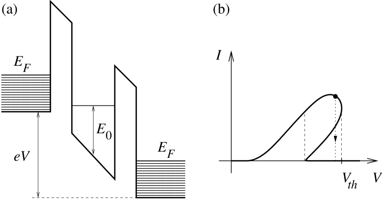
Figure 1: (a) The potential profile of the DBRTS at applied bias $V$. (b) The $I$-$V$ curve of the device has a bistable region between the dashed lines. The dotted line shows the process of switching from a metastable state to the stable one.

We concentrate on the case of intrinsic bistability, which can be observed by measuring current $I$ as a function of voltage $V$ applied to the device while the impedance of the external circuit equals zero. As shown in Ref. Goldman:exp, , for a certain range of bias $V$, two states of current $I$ are possible at the same value of the voltage, and the $I$-$V$ curve has characteristic hysteretic behavior. As one increases bias, the upper branch ends at some boundary voltage $V_{th}$, shown schematically in Fig. 1(b). If the voltage $V$ is fixed just below the threshold $V_{th}$, the system stays in the upper state for a finite time $\tau$, before decaying to the stable lower state.

We will show that the lifetime of the metastable state $\tau$ can be understood by analogy to the problem of a Brownian particle in a double-well potential (Fig. 2). Here the coordinate of the Brownian particle has the meaning of the current $I$ in the device (or the electron density $n$). In the problem of the Brownian particle, $\tau$ depends exponentially on the height of the potential barrier $U_{b}$ separating the local and global minima, i.e. $\tau\propto{\exp(U_{b}/T^{\ast})}$, where $T^{\ast}$ is the temperature. Unlike a Brownian particle, a DBRTS at nonzero bias is a non-equilibrium system in which fluctuation phenomena are driven by shot noise in the current rather than the electron temperature $T$. On the boundary of the bistable region, the local minimum disappears, and therefore $U_{b}$ goes to zero. Thus, it is clear that $\tau$ will depend exponentially on the voltage measured from the boundary $V_{th}$ of the bistable region.

Here we investigate effects of shot noise in DBRTS using the framework of the theoretical model introduced in Ref. Blanter99, . The DBRTS is formed as a layered semiconductor heterostructure. The electrostatic potential across the device is shown in Fig. 1(a). The potential is assumed to be independent of the $x$ and $y$ coordinates. The model includes only one subband in the quantum well. We furthermore assume that at zero bias the bottom of this subband $E_{0}$ is above the Fermi energy $E_{F}$ in the left and right leads. If the area of the sample $S$ is small, we can assume that the charge in the well is distributed uniformly. Then, the state of the device is completely described by the electron density $n$ in the quantum well. Below we will also discuss effects of non-uniform charge distribution in the well, which are important in the case of devices of large area.

In the sequential tunneling approximation, the transport in the device is described by the following master equation for the time-dependent distribution function $P(n,t)$ of the electron density $n$ in the well,

$$\frac{\partial P(n,t)}{\partial t} = P\left(n-\frac{1}{S},t\right)\sum_{{\bf qk}}W_{\bf kq}\left(n-\frac{1}{S}\right)f_{\bf k}(1-f_{\bf q})$$ (1)

$$+P\left(n+\frac{1}{S},t\right)\sum_{{\bf qp}}W_{\bf qp}\left(n+\frac{1}{S}\right)f_{\bf q}$$

$$-P(n,t)\sum_{{\bf qk}}W_{\bf kq}(n)f_{\bf k}(1-f_{\bf q})$$

$$-P(n,t)\sum_{{\bf qp}}W_{\bf qp}(n)f_{\bf q}.$$

Here $f_{\bf k}$, $f_{\bf p}$, and $f_{\bf q}$ are the Fermi occupation numbers in the left lead, right lead, and the quantum well, respectively; $W_{\bf kq}(n)$ and $W_{\bf qp}(n)$ are the tunneling rates through the left and right barriers. The first two terms of Eq. (1) account for the processes which bring the system to the state of electron density $n$, and the last two terms describe the processes that take the system away from it. The first and the third terms on the right-hand side of Eq. (1) describe tunneling of one electron into the well from the left lead, while the second and the fourth ones account for the probability of an electron in the quantum well to tunnel into the right lead. We dropped the terms describing the tunneling from the well to the left lead and tunneling from the right lead into the well. These contributions are negligible because the bistability emerges Blanter99 when the level in the well is close to the bottom of the conduction band in the left lead and far above the Fermi level in the right lead. (We assume $T\ll E_{F}$.)

Figure 2: Brownian particle in a double-well potential. The lifetime of the metastable state $\tau$ depends exponentially on the height of the barrier $U_{b}$ separating the local and global minima, $\tau\propto\exp(U_{b}/T^{\ast})$. The coordinate of the particle $x$ has the meaning of the electron density $n$ in the well, and $U(n)=Su(n)$, see Eq. (3).

Assuming that the total number of particles in the well is large, $nS\gg 1$, we can expand (1) in the small parameter $1/S$. Keeping terms up to the second order we reduce the master equation to the Fokker-Planck equation,

$$\frac{\partial P(n,t)}{\partial t}=-\frac{\partial}{\partial n}[A(n)P(n,t)]+\frac{1}{2}\frac{\partial^{2}}{\partial n^{2}}[B(n)P(n,t)].$$ (2)

The exact expressions for $A(n)$ and $B(n)$ are rather complicated, but near the threshold they can be calculated analytically, see Eq. (4) below.

The stationary solution of Eq. (2) can be easily obtained:

$$P_{0}(n)=\frac{\mbox{const}}{B(n)}e^{-Su(n)},\quad u(n)=-\frac{2}{S}\int_{0}^{n}\frac{A(n^{\prime})}{B(n^{\prime})}\,dn^{\prime},$$ (3)

where $u(n)$ is the effective potential.

In the derivation of the Fokker-Planck equation (2), the coefficients $A(n)$ and $B(n)$ appeared as the first and second terms of the expansion in $1/S$. We therefore conclude that $A(n)/B(n)\propto S$, and $u(n)$ is independent of $S$. Thus when the area $S$ is large, the distribution function $P_{0}(n)$ has very narrow peaks near the minima of $u(n)$. If we neglect the fact that the width is finite, then the electron density $n$ in the well can be found by minimizing $u(n)$. The minimization condition written as $A(n)=0$ is in agreement with the results of Ref. Blanter99, .

Our model allows for an analytical treatment at small values of the parameter $\lambda={m{e}^{2}}/{2\pi{\hbar}^{2}C}$, where $C$ is the capacitance of the device per unit area. Then the calculations are greatly simplified, and one obtains the following expressions for $A$ and $B$ near the threshold:

$$A(n) = -\frac{b}{2}\left[-\alpha+\gamma(n-n_{th})^{2}\right],$$ (4a)

$$b \equiv SB(n_{th})=\frac{\sqrt{2}}{\pi}\lambda^{2}\frac{T_{L}^{2}}{T_{R}}\frac{C}{e^{2}}E_{F}^{2},$$ (4b)

$$\alpha = 2\frac{1}{\lambda^{2}}\left(\frac{T_{R}}{T_{L}}\right)^{2}\frac{E_{0}}{E_{F}^{2}}e\,\delta V,$$ (4c)

$$\gamma = 2\frac{1}{\lambda^{4}}\left(\frac{T_{R}}{T_{L}}\right)^{4}\left(\frac{e^{2}}{C}\right)^{2}\frac{E_{0}^{2}}{E_{F}^{4}}.$$ (4d)

Here $\delta V=V_{th}-V$, the electron density at the threshold $n_{th}=\frac{\lambda^{2}}{2}\left(\frac{T_{L}}{T_{R}}\right)^{2}\frac{CE_{F}^{2}}{e^{2}E_{0}}$; and $T_{L,R}$ are the transmission coefficients of the left and right barriers at energy $E_{0}$ and zero applied bias. If $\lambda$ is not small, we cannot get explicit expressions for $\alpha$, $\gamma$ and $b$, but the generic form of Eq. (4a) remains unchanged.

The potential $u(n)$ is shown schematically in Fig. 2 for a voltage which lies slightly below the threshold voltage $V_{th}$. Close to the threshold the potential can be approximated by a cubic polynomial,

$$u(n)\approx-\alpha(n-n_{th})+\frac{\gamma}{3}(n-n_{th})^{3}+u(n_{th}).$$ (5)

Taking into account the exponential dependence of the mean switching time on the barrier height, $\tau=\tau_{0}e^{U_{b}}$, and using Eq. (5), we find

$$\ln\frac{\tau}{\tau_{0}}=\frac{4}{3}\frac{S\alpha^{3/2}}{\gamma^{1/2}}\propto S\,\delta V^{3/2}.$$ (6)

The prefactor $\tau_{0}$ can be found using the techniques described, e.g., in Ref. vanKampen, .

It is important to note that the form (5) of the potential $u(n)$ and the linear dependence $\alpha\propto\delta V$ are dictated by analyticity of the potential near the threshold. Thus, the applicability of the following results is not limited to a particular model of transport in DBRTS. A $3/2$-power law analogous to Eq. (6) was theoretically predicted for different physical systems in Refs. Kurkijarvi ; Victora ; Dykman1 ; Dykman2 . Experimentally it was observed recently for an optically trapped Brownian particle Dykman:exp .

The result (6) has been obtained under the assumption that the electrons spread rapidly in the $x$-$y$ plane, and their density $n$ is uniform. In large samples, however, the spreading takes a long time, and one has to account for the dependence of the density $n$ on the point ${\bf r}=(x,y)$ in the well. This can be done by generalizing the Fokker-Planck equation (2) to the case of non-uniform ${n({\bf r})}$.

We begin by studying the in-plane diffusion of electrons in the well neglecting coupling to the leads. For simplicity we neglect the electron correlation effects; the interactions of electrons will be accounted for in the charging energy approximation. Assuming that the electrons diffuse independently, one can write a master equation for the distribution function $P\{n({\bf r}),t\}$ as follows. During the time $\Delta t$ at most one electron can move from position ${\bf r}_{1}$ to ${\bf r}_{2}$, that is,

$$P\{n({\bf r}),t+\Delta t\}-P\{n({\bf r}),t\}=\int\!\!\int d{\bf r}_{1}d{\bf r}_{2}$$

$$\times\Big{[}P\{n({\bf r})+\delta({\bf r}-{\bf r}_{1})-\delta({\bf r}-{\bf r}_{2}),t\}W({\bf r}_{1},{\bf r}_{2},\Delta t)$$

$$-P\{n({\bf r}),t\}W({\bf r}_{2},{\bf r}_{1},\Delta t)\Big{]}.$$ (7)

Here $W({\bf r}_{1},{\bf r}_{2},\Delta t)$ is the probability density of an electron diffusing from a point ${\bf r}_{1}$ in the plane of the quantum well to point ${\bf r}_{2}$ during the time interval $\Delta t$. Since electrons are fermions, a particle can diffuse only from a filled state at ${\bf r}_{1}$ to an empty state at ${\bf r}_{2}$. Assuming that the diffusion is due to the elastic scattering of electrons by defects, we find

$$W({\bf r}_{1},{\bf r}_{2},\Delta t)=g({\bf r}_{1}-{\bf r}_{2},\Delta t)\nu\int f_{1}(E)[1-f_{2}(E)]\,dE,$$ (8)

where $\nu$ is the density of states in the well (per unit area), and $f_{1,2}(E)$ are the occupation numbers at points ${\bf r}_{1}$, ${\bf r}_{2}$. The classical diffusion probability $g(r,\Delta t)$ is given by

$$g({\bf r},\Delta t)=\frac{1}{4\pi D\Delta t}e^{-{\bf r}^{2}/{4D\Delta t}}\simeq\delta({\bf r})+D\Delta t\nabla^{2}\delta({\bf r}),$$ (9)

where $D$ is the diffusion coefficient. The approximate form is obtained in the limit $\Delta t\to 0$.

Using Eqs. (8), (9) and expanding the distribution function from Eq. (7) up to the second order in $\delta({\bf r}-{\bf r}_{1})-\delta({\bf r}-{\bf r}_{2})$ we obtain a functional Fokker-Planck equation,

$$\frac{\partial P\{n({\bf r}),t\}}{\partial t}=\nu D\int\!\!\int d{\bf r}_{1}d{\bf r}_{2}$$

$$\times\left[\left(\frac{\delta}{\delta n({\bf r}_{1})}-\frac{\delta}{\delta n({\bf r}_{2})}\right)+\frac{1}{2}\left(\frac{\delta}{\delta n({\bf r}_{1})}-\frac{\delta}{\delta n({\bf r}_{2})}\right)^{2}\right]$$

$$\times\frac{\mu_{1}-\mu_{2}}{1-e^{-(\mu_{1}-\mu_{2})/T}}P\{n({\bf r}),t\}\nabla^{2}\delta({\bf r}_{1}-{\bf r}_{2}).$$ (10)

Here $\mu_{1}$ and $\mu_{2}$ are the electrochemical potentials at ${\bf r}_{1}$ and ${\bf r}_{2}$, respectively. Their values are found by adding the electrostatic potential $e^{2}n/C$ to the Fermi energy $n/{\nu}$,

$$\mu_{1,2}=\frac{e^{2}}{\tilde{C}}n({\bf r}_{1,2}).$$ (11)

Here $\tilde{C}$ is defined by $e^{2}/{\tilde{C}}=e^{2}/{C}+1/{\nu}$.

Substituting Eq. (11) into Eq. (Lifetime of metastable states in resonant tunneling structures), integrating twice by parts and assuming that $|\mu_{1}-\mu_{2}|\ll T$, one obtains the following Fokker-Planck equation,

$$\frac{\partial P\{n,t\}}{\partial t}=-\nu D\int d{\bf r}\frac{\delta}{\delta n}\left[\frac{e^{2}}{\tilde{C}}\nabla^{2}n+T\nabla^{2}\frac{\delta}{\delta n}\right]P\{n,t\}.$$ (12)

The stationary solution of Eq. (12) is found easily by requiring the part of the integrand after the first functional derivative to vanish,

$$P_{0}\{n\}=\exp\left[-\frac{1}{T}\int\frac{e^{2}n^{2}({\bf r})}{2\tilde{C}}\,d{\bf r}\right].$$

This result has a simple physical meaning. The equilibrium distribution function $P_{0}$ has the Gibbs form $e^{-E/T}$, with the energy per unit area ${e^{2}n^{2}}/{2{\tilde{C}}}$ in agreement with the electrochemical potential (11).

Using Eq. (12) we can take into account processes of charge spreading in the quantum well. The electron density $n({\bf r})$ can change due to either tunneling of electrons through the barriers or their diffusion inside the well. Thus, we must add the terms from the right-hand side of Eq. (2) to Eq. (12) to account for both processes. The combined Fokker-Planck equation takes the form

$$\frac{\partial P\{n({\bf r}),t\}}{\partial t} = \int d{\bf r}\frac{\delta}{\delta n}\left[-A(n)+\frac{S}{2}\frac{\delta}{\delta n}B(n)\right.$$ (13)

$$\left.-\nu D\frac{e^{2}}{\tilde{C}}\nabla^{2}n\right]P\{n({\bf r}),t\}.$$

Here we neglected the second term in Eq. (12). This can be done as long as the temperature of the electrons in the well is much lower than the Fermi energy .

The stationary solution of this equation is

$$P_{0}\{n\}=\frac{\mbox{const}}{B(n)}e^{-F},\quad F\{n\}=\int d{\bf r}\left[u(n)+\eta(\nabla n)^{2}\right],$$ (14)

where $\eta=\nu De^{2}/{\tilde{C}}SB(n)$. Note that in the limit $D\to\infty$ the electron density is uniform, $\nabla n=0$, and we recover the result (3).

In the case when the diffusion coefficient $D$ is finite, the electron density varies from point to point in the quantum well; hence, this problem is infinite dimensional. In the multi-dimensional case, the system escapes from the local minimum of potential through a point where the barrier separating it from the global minimum takes the lowest possible value, i.e., through a saddle point. The mean switching time $\tau$ is determined by the potential at the saddle point, measured from the local minimum. This approach is similar to the one used in the theory of kinetics of first-order phase transitions Langer , with $F$ playing the role of the free energy.

The saddle point of the functional $F\{n\}$ is achieved at $n=n_{s}({\bf r})$ which almost everywhere in the sample is very close to the density $n_{min}$ of the system at the local minimum of $F$. However, in a region of some characteristic size $r_{0}$, the density $n_{s}({\bf r})$ changes in the direction of the global minimum, Fig. 2. Thus, the DBRTS of large area first switches to the stable state in a region of size $r_{0}$, which then expands to the whole sample.

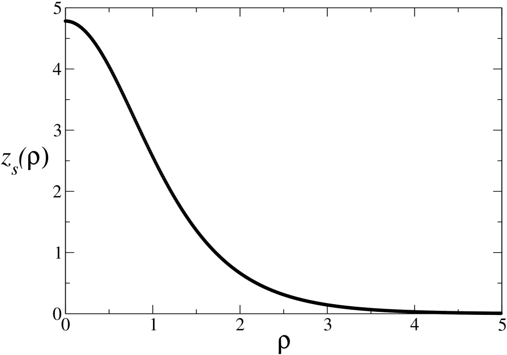
Figure 3: Numerical solution of Eq. (15).

We perform the following calculations in the regime of voltages very close to the threshold $V_{th}$, where we can use $u(n)$ in the form (5), and $\eta$ takes a constant value $\eta=\nu De^{2}/{\tilde{C}}b$. Initially the system is in the local minimum, described by a uniform density $n_{min}=n_{th}+\sqrt{{\alpha}/{\gamma}}$. In order to find the saddle point, it is convenient to parametrize the electron density $n({\bf r})$ in terms of a dimensionless function $z(\bm{\rho})$, such that $n({\bf r})=n_{min}-\sqrt{{\alpha}/{\gamma}}\,z({\bf r}/{r_{0}})$, where the length scale $r_{0}=\sqrt{2\eta}\,(\alpha\gamma)^{-1/4}$. Using this parametrization, one can find the saddle point of $F$ as a non-trivial solution $z_{s}(\bm{\rho})$ of the equation

$$-\nabla^{2}z+2z-z^{2}=0,$$ (15)

with the boundary condition $z_{s}(\bm{\rho})=0$ at $\rho\rightarrow\infty$. It can be obtained numerically, Fig. 3.

The switching rate $\tau^{-1}$ is proportional to the distribution function $P_{0}\{n_{s}\}$, where $n_{s}({\bf r})=n_{min}-\sqrt{{\alpha}/{\gamma}}\,z_{s}({\bf r}/{r_{0}})$. Therefore, one can calculate the logarithm of the mean switching time $\tau$ as $F\{n_{s}\}-F\{n_{min}\}$,

$$\ln\frac{\tau}{\tau_{2}}=\kappa\frac{\alpha\eta}{\gamma}\propto\delta V.$$ (16)

Here the constant $\kappa\simeq 62.01$ was found numerically .

According to Eq. (16), $\ln\frac{\tau}{\tau_{2}}$ does not depend on the area $S$. On the other hand, since the critical fluctuation $n_{s}({\bf r})$ can be centered anywhere in the sample, the switching rate $\tau^{-1}$ is proportional to the area of the sample $S$, hence $\tau_{2}\propto 1/S$. The exact calculation of the prefactor $\tau_{2}$ presents a number of theoretical challenges, which we leave for future work.

In contrast to the case of small samples Eq. (6), the logarithm of the escape time (16) in large samples is linear in $\delta V$. The crossover between the two regimes occurs when the area $S$ of the sample is of the order of $r_{0}^{2}=2\eta(\alpha\gamma)^{-1/2}$. One can see from Eq. (4c) that $r_{0}^{2}\propto\delta V^{-1/2}$. Thus, one can observe this crossover in a single sample by tuning the voltage. Indeed, at relatively small $\delta V$ we will have $S\ll r_{0}^{2}$ and $\ln\tau\propto\delta V^{3/2}$, Eq. (6), whereas at larger $\delta V$ we have $\ln\tau\propto\delta V$, Eq. (16).

In conclusion, we have studied the switching time $\tau$ from the metastable state to the stable one in DBRTS. We showed that $\tau$ is exponential in the voltage measured from the boundary of the bistable region; it is given by Eq. (6) or (16) depending on the area of the sample. Our results can be tested in experiments similar to Refs. Teitsworth, ; Grahn, .

We are grateful to M. I. Dykman, H. T. Grahn and S. W. Teitsworth for valuable discussions. T. G. acknowledges support from the Swiss National Science Foundation. This work was also supported by the NSF Grants DMR-9974435 and DMR-0214149 and by the Sloan foundation.

References

- (1) J. S. Langer, Ann. Phys. 41, 108 (1967).
- (2) J. Kurkijärvi, Phys. Rev. B 6, 832 (1972).
- (3) S. Coleman, Aspects of Symmetry (Cambridge University Press, Cambridge, 1985), Ch.7 and Refs. therein.
- (4) R. H. Victora, Phys. Rev. Lett. 63, 457 (1989).
- (5) M. I. Dykman, E. Mori, J. Ross, and P. M. Hunt, J. Chem. Phys. 100, 5735 (1994).
- (6) V. J. Goldman, D. C. Tsui, and J. E. Cunningham, Phys. Rev. Lett. 58, 1256 (1987).
- (7) J. Kastrup, H. T. Grahn, K. Ploog, F. Prengel, A. Wacker, and E. Schöll, Appl. Phys. Lett. 65, 1808 (1994).
- (8) M. Rogozia, S. W. Teitsworth, H. T. Grahn, and K. H. Ploog, Phys. Rev. B 64, 041308(R) (2001).
- (9) K. J. Luo, H. T. Grahn, and K. H. Ploog, Phys. Rev. B 57, R6838 (1998).
- (10) Ya. M. Blanter and M. Büttiker, Phys. Rev. B 59, 10217 (1999).
- (11) N. G. van Kampen, Stochastic Processes in Physics and Chemistry (Elsevier, Amsterdam, 1992), Sec. VIII.2.
- (12) M. I. Dykman and M. A. Krivoglaz, Physica A 104, 480 (1980).
- (13) M. I. Dykman, B. Golding, J. R. Kruse, L. I. McCann and Ryvkine, cond-mat/0204621.
- (14) K. G. Selivanov, Sov. Phys. JETP, 67, 1548 (1988).