Second Law in Classical Non-Extensive Systems

Abstract

Equilibrium statistics of Hamiltonian systems is correctly described by the microcanonical ensemble, whereas canonical ones fail in the most interesting, mostly inhomogeneous, situations like phase separations or away from the “thermodynamic limit” (e.g. self-gravitating systems and small quantum systems) [1, 2, 3]. A new derivation of the Second Law is presented that respects these fundamental complications. Our “geometric foundation of Thermo-Statistics” [3] opens the fundamental (axiomatic) application of Thermo-Statistics to non-diluted systems or to “non-simple” systems which are not similar to (homogeneous) fluids. Supprisingly, but also understandably, a so far open problem c.f. ref. [4] page 50 and page 72.

1 Introduction

Phase separation of normal systems and also the equilibrium of closed non-extensive systems are not described by the canonical and grand-canonical ensembles. Only the microcanonical ensemble based on Boltzmann’s principle $S=\ln{W}$, with $W(E)=\epsilon_{0}tr[\delta(E-H)]$, the classical or quantum number of states, describes correctly the unbiased uniform filling of the energy-shell in phase-space.

The various ensembles are equivalent only if the system is infinite and homogeneous, i.e. in a pure phase. As this conference addresses the Second Law in quantum systems (i.e. small systems) and moreover, as most systems in nature are inhomogeneous it seems necessary to take the above complication serious. We should deduce the Second Law from reversible mechanics without invoking the thermodynamic limit ($\lim_{V\to\infty,N/V=\rho}$) and using the microcanonical ensemble with sharply defined conserved quantities.

2 Boltzmann’s principle, the microcanonical ensemble

The key quantity of statistics and thermodynamics is the entropy $S$. Its most fundamental definition is as the logarithm of the area $W(E)$ of the manifold $\cal{E}$ in the N-body phase-space given by Boltzmann’s principle [5]:

$$W(E,N,V) = \epsilon_{0}tr\delta(E-H_{N})$$

$$tr\delta(E-H_{N}) = \int{\frac{d^{3N}p\;d^{3N}q}{N!(2\pi\hbar)^{3N}}\delta(E-H_{N})}.$$ (1)

S=k lnW (2)

Boltzmann’s principle is the only axiom necessary for thermo-statistics. With it Statistical Mechanics and also Thermodynamics become geometric theories[3]. For instance all kinds of phase-transitions are entirely determined by topological peculiarities of the ($6N-1$)-dim. manifold ${\cal{E}}(E,N,\cdots)$ of all points in the $6N$-dim. phase space with given energy $E$, particle number $N$ etc. More precisely, the topology of $S(E,N,\cdots)$ determines the thermodynamic properties of the system including all its phase-transitions [1, 2].

3 Approach to equilibrium, Second Law

3.1 Zermelo’s paradox

When Zermelo [6] argued against Boltzmann, that following Poncarré any many-body system must return after the Poincarré recurrence time $t_{rec}$ and consequently its entropy cannot always grow, but must decay also, Boltzmann [7] answered that for any macroscopic system $t_{rec}$ is of several orders of magnitude larger than the age of the universe, c.f. Gallavotti [8]. Still today, this is the answer given when the Second Law is to be proven microscopically, c.f. [9]. I.e. the thermodynamic limit seems necessary for the validity of the Second Law [10, 11]. Then, however, Zermelo’s paradox becomes blunted.

However, the reason for the Second Law is not the large recurrence times but the probabilistic nature of Thermodynamics. Here, I argue, even a small system approaches equilibrium with a rise of its entropy $\Delta S\geq 0$ under quite general conditions. Thus, Zermelo’s objection must be considered much more seriously.

However, care must be taken, Boltzmann’s definition of entropy eq.(2) is only for systems at equilibrium. To be precise: in the following I will consider the equilibrium manifold ${\cal{M}}(t)={\cal{E}}(E,V_{a})$ at $t\leq t_{0}$. At $t_{0}$ the macroscopic constraint $V_{a}$ is quickly removed e.g. a piston pulled quickly out to $V_{a}+V_{b}$, and the ensemble is followed in phase-space how it approaches the new equilibrium manifold ${\cal{E}}(E,V_{a}+V_{b})$ see fig.(1).

3.2 The solution

Due to the reduced, incomplete, description of a $N$-body system by Thermodynamics does entropy not refer to a single point in $N$-body phase space but to the whole ensemble ${\cal{E}}$ of points. It is the $\ln(W)$ of the geometrical size $W$ of the ensemble. Every trajectory starting at different points in the initial manifold ${\cal{M}}(t=t_{0})={\cal{E}}(E,V_{a})\in{\cal{E}}(E,V_{a}+V_{b})$ spreads in a non-crossing manner over the available phase-space ${\cal{E}}(E,V_{a}+V_{b})$ but returns after $t_{rec}$. Different points of the manifold, or trajectories, have different $t_{rec}$ which are normally incommensurable. I.e. the manifold ${\cal{M}}(t>t_{0})$ spreads irreversibly over ${\cal{E}}(E,V_{a}+V_{b})$. ${\cal{M}}(t)$ will never go back into the volume $V_{a}$.

3.2.1 Mixing

When the system is dynamically mixing then the manifold ${\cal{M}}(t)$ will “fill” the new ensemble ${\cal{E}}(E,V_{a}+V_{b})$. Though at finite times the manifold remains compact due to Liouville and keeps the volume $W(E,V_{a})$, but as already argued by Gibbs [12, 13] ${\cal{M}}(t)$ will be filamented like ink in water and will approach any point of ${\cal{E}}(E,V_{a}+V_{b})$ arbitrarily close. Then, $\lim_{t\to\infty}{\cal{M}}(t)$ becomes dense in the new, larger ${\cal{E}}(E,V_{a}+V_{b})$.

3.2.2 Macroscopic resolution, fractal distributions and closure [14]

Also an idealized mathematical analysis is possible here: Statistical Mechanics as a probabilistic theory describes all systems in the same volume $V$ and with the same few conserved control parameters like energy $E$, particle number $N$ etc. It is unable to distinguish the points $\in M(t)$ from the neighboring points in its closure $\overline{{\cal{M}}(t)}$. Entropy is also the $\ln$ of the size of $\overline{{\cal{M}}(t)}$. The closure $\overline{{\cal{M}}(t=\infty)}$ becomes equal to ${\cal{E}}(E,V_{a}+V_{b})$. I.e. the entropy $S(t=\infty)>S(t_{0})$. This is the Second Law for a finite system.

We calculate the closure of the ensemble by box counting [15]. Here the phase-space is divided in $N_{\delta}$ equal boxes of volume $\delta^{6N}$. The number of boxes which overlap with ${\cal{M}}(t)$ is $N_{\delta}$ and the box-counting volume is then:

$$\Omega_{d}(\delta) = N_{\delta}\delta^{d}$$

here with $$d=6N-1$$

$$\Omega_{d} = \lim_{\delta\to 0}\Omega_{d}(\delta).$$ (4)

The box-counting method is illustrated in fig.(1). The important aspect of the box-counting volume of a manifold is that it is equal to the volume of its closure.

At finite times ${\cal{M}}(t)$ is compact. Its volume $W(t)$ equals that of its closure $\equiv W(t_{0})$. However, calculated with finite resolution $\delta>0$, $W_{\delta}(t)$ becomes $\geq W(t)$ for $t$ larger than some $t_{\delta}$, where

$$W_{\delta}(t) =$$

$$\displaystyle{B_{d}^{\delta}\int}\;\;\frac{d^{3N}p_{t}\;d^{3N}q_{t}}{(2\pi\hbar)^{3N}}\;\delta\left(E-H_{N}\{q(t),p(t);\}\right)$$ (5)

$$\mbox{with the constraint }[q(t_{0}),p(t_{0})\in{\cal{E}}(V_{a})]$$

and the definition:

$$\displaystyle{B_{d}^{\delta}\int}{\;\;f(q)d^{d}q} := \Omega_{d}(\delta)\overline{f(q)}.$$

A natural finite resolution is given by Quantum Mechanics:

$$\delta=\sqrt{2\pi\hbar},$$ (6)

but Thermodynamics allows a much coarser resolution because of the insensitivity of the usual macroscopic observables. Then the equilibration time $t_{\delta}$ will also be much shorter.

$V_{a}$                 $V_{b}$

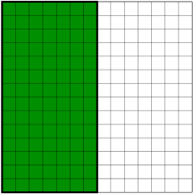
$t<t_{0}$

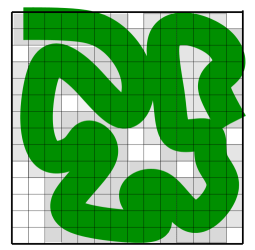
$\longrightarrow$ $V_{a}+V_{b}$ $t>t_{0}$

Figure 1: The compact set ${\cal{M}}(t_{0})={\cal{E}}(V_{a})$, left side, develops into an increasingly folded but non-crossing “spaghetti”-like distribution ${\cal{M}}(t)$ in the phase-space with rising time $t$ after opening the volume $V_{b}$. The right figure shows only the early form of the distribution. At much later times it will become more and more fractal and finally dense in the new larger phase space. The grid illustrates the boxes of the box-counting method. All boxes which overlap with ${\cal{M}}(t)$ contribute to the box-counting volume and are shaded gray. Their number is $N_{\delta}$

Thus we should reformulate Boltzmann’s principle eqs. (2) as:

$$S(t)=\ln(W_{\delta}(t)),$$ (7)

or mathematically correct, though unphysical, at infinite times:

$$S(t\to\infty) = \lim_{\delta\to 0}\lim_{t\to\infty}{\ln(W_{\delta}(t))}$$ (8)

$$= N\ln[(V_{a}+V_{b})/V_{a}]+S(t_{0}),$$

which agrees with the old one eq. (2) for compact manifolds like ${\cal{E}}$.

4 Conclusion

The geometric interpretation of classical equilibrium Statistical Mechanics [3] by Boltzmann’s principle offers an extension also to the equilibrium of non-extensive systems. In more fundamental, axiomatic terms, it opens the application of Thermo-Statistics to “non-simple” systems which are not similar to fluids or systems in contact with an ideal gas. Surprisingly, but also understandably, this is a so far open problem c.f. ref. [4] page 50 and page 72.

Because microcanonical Thermodynamics as a macroscopic theory controls the system by a few, usually conserved, macroscopic parameters like energy, particle number, etc. it is an intrinsically probabilistic theory. It describes all systems with the same control-parameters simultaneously. If we take this seriously and avoid the so called thermodynamic limit ($\lim_{V\to\infty,N/V=\rho}$), the theory can be applied to small systems like the usual quantum systems addressed in this conference but even to the really large, usually inhomogeneous, self-gravitating systems, c.f.[16].

Within the new, extended, formalism several principles of traditional Statistical Mechanics turn out to be violated and obsolete. E.g. at phase-separation heat (energy) can flow from cold to hot [1]. Or phase-transitions can be classified unambiguously in astonishingly small systems. These are by no way exotic and wrong conclusions. On the contrary, many experiments have shown their validity. I believe this approach gives a much deeper insight into the way how many-body systems organize themselves than any canonical statistics is able to. The thermodynamic limit clouds the most interesting region of Thermodynamics, the region of inhomogeneous phase-separation.

Relevant for most of the contributions to this conference is the fact that the various canonical ensembles are not equivalent to the fundamental microcanonical one. They fail to describe the equilibrium of small systems like quantum systems, as well the largest systems possible like self-gravitating ones, or the thermodynamical most important situations like phase-separation with their negative heat-capacity [1].

Because of the only one underlying axiom, Boltzmann’s principle eq.(2 or 7), the geometric interpretation [3] keeps statistics most close to Mechanics and, therefore, is most transparent. The Second Law ($\Delta S\geq 0$) is shown to be valid in closed, small systems under quite general dynamical conditions.

One may consider this as an artificial mathematical construct, far away from our daily experience about temperature, heat etc. However, it must be emphasized that in the usual macroscopic, extensive world nothing changes. The change of entropy is still the change of heat over temperature: $dS=dQ/T$. However, the application of Thermodynamics to unusual systems like quantum systems or non-extensive systems demands an abstract mathematical extension like the one proposed here.

References

- [1] Gross, D., “Thermo-Statistics or Topology of the Microcanonical Entropy Surface”, in Dynamics and Thermodynamics of Systems with Long Range Interactions, edited by T.Dauxois, S.Ruffo, E.Arimondo, and M.Wilkens, Springer, Heidelberg, 2002, Lecture Notes in Physics, pp. 21–45,cond–mat/0206341.
- [2] Gross, D., Microcanonical thermodynamics: Phase transitions in “Small” systems, vol. 66 of Lecture Notes in Physics, World Scientific, Singapore, 2001.
- [3] Gross, D., PCCP, 4, 863–872,http://arXiv.org/abs/cond–mat/0201235 ((2002)).
- [4] Uffink, J., cond-mat/0005327.
- [5] Einstein, A., Annalen der Physik, 17, 132 (1905).
- [6] Zermelo, E., Wied.Ann., 60, 392–398 (1897).
- [7] Boltzmann, L., “Entgegnung auf die wärmetheoretischen Betrachtungen des Hrn.E. Zermelo”, in Kinetic Theory, edited by S. Brush, Pergamon Press, Oxford, 1965-1972, 2, p. 218.
- [8] Gallavotti, G., Statistical Mechanics, Texts and Monographs in Physics, Springer, Berlin, 1999.
- [9] Gaspard, P., J.Stat.Phys, 88, 1215–1240 (1997).
- [10] Lebowitz, J., Physica A, 263, 516–527 (1999).
- [11] Lebowitz, J., Rev.Mod.Phys., 71, S346–S357 (1999).
- [12] Gibbs, J., Elementary Principles in Statistical Physics, vol. II of The Collected Works of J.Willard Gibbs, Yale University Press 1902,also Longmans, Green and Co, NY, 1928.
- [13] Gibbs, J., Collected works and commentary,vol I and II, Yale University Press, 1936.
- [14] Gross, D., “Ensemble probabilistic equilibrium and non-equilibrium thermodynamics without the thermodynamic limit”, in Foundations of Probability and Physics, edited by A. Khrennikov, ACM, World Scientific, Boston, 2001, PQ-QP: Quantum Probability, White Noise Analysis XIII, pp. 131–146.
- [15] Falconer, K., Fractal Geometry - Mathematical Foundations and Applications, John Wiley & Sons, Chichester, New York, Brisbane, Toronto,Singapore, 1990.
- [16] Votyakov, E., Hidmi, H., Martino, A. D., and Gross, D., Phys.Rev.Lett., 89, 031101–1–4; http://arXiv.org/abs/cond–mat/0202140 (2002)).